www.atmos-chem-phys.net/16/2299/2016/ doi:10.5194/acp-16-2299-2016
© Author(s) 2016. CC Attribution 3.0 License.
Change in turbopause altitude at 52 and 70
◦
N
Chris M. Hall1, Silje E. Holmen1,2,5, Chris E. Meek3, Alan H. Manson3, and Satonori Nozawa4
1Tromsø Geophysical Observatory, UiT – The Arctic University of Norway, Tromsø, Norway 2The University Centre in Svalbard, Svalbard, Norway
3University of Saskatchewan, Saskatoon, Canada 4Nagoya University, Nagoya, Japan
5Birkeland Centre for Space Science, Bergen, Norway Correspondence to:Chris M. Hall ([email protected])
Received: 5 May 2015 – Published in Atmos. Chem. Phys. Discuss.: 24 July 2015 Revised: 22 January 2016 – Accepted: 10 February 2016 – Published: 26 February 2016
Abstract.The turbopause is the demarcation between atmo-spheric mixing by turbulence (below) and molecular diffu-sion (above). When studying concentrations of trace species in the atmosphere, and particularly long-term change, it may be important to understand processes present, together with their temporal evolution that may be responsible for redis-tribution of atmospheric constituents. The general region of transition between turbulent and molecular mixing coincides with the base of the ionosphere, the lower region in which molecular oxygen is dissociated, and, at high latitude in sum-mer, the coldest part of the whole atmosphere.
This study updates previous reports of turbopause altitude, extending the time series by half a decade, and thus shedding new light on the nature of change over solar-cycle timescales. Assuming there is no trend in temperature, at 70◦N there is evidence for a summer trend of ∼1.6 km decade−1, but for winter and at 52◦N there is no significant evidence for change at all. If the temperature at 90 km is estimated us-ing meteor trail data, it is possible to estimate a coolus-ing rate, which, if applied to the turbopause altitude estimation, fails to alter the trend significantly irrespective of season.
The observed increase in turbopause height supports a hy-pothesis of corresponding negative trends in atomic oxygen density, [O]. This supports independent studies of atomic oxygen density, [O], using mid-latitude time series dating from 1975, which show negative trends since 2002.
1 Introduction
win-ter mesosphere, whereas in summer the gravity waves “save their energy” more until reaching the “steep beach” (a vi-sualisation attributable to M. E. McIntyre, personal commu-nication, 1988) of the summer mesopause near 85 km. Ver-tical transport by turbulent mixing and horizontal transport by winds redistribute constituents such as atomic oxygen, hydroxyl and ozone. Thus, long-term change in trace con-stituents cannot be fully explained in isolation from studies of corresponding change in temperature and neutral dynam-ics.
One means of locating the turbopause is to measure the concentration of particular species as a function of height and noting where the constituents exhibit scale heights that depend on their respective molecular weights (e.g. Danilov et al., 1979). Detection of turbulence and estimation of its intensity is non-trivial because direct measurement by radar depends on turbulent structures being “visible” due to small discontinuities in refractive index (e.g. Schlegel et al., 1978, and Briggs, 1980). At 100 km, this implies some degree of ionisation and even in situ detectors often depend on ionisa-tion as a tracer (e.g. Thrane et al., 1987). A common means of quantifying turbulent intensity is the estimation of tur-bulent energy dissipation rate, ε. In the classical visualisa-tion of turbulence in two dimensions, large vortices gener-ated by, for example, breaking gravity waves or wind shears form progressively smaller vortices (eddies) until inertia is insufficient to overcome viscous drag in the fluid. Viscosity then “removes” kinetic energy and transforms it to heat. This “cascade” from large-scale vortices to the smallest-scale ed-dies capable of being supported by the fluid, and subsequent dissipation of energy, was proposed by Kolmogorov (1941) but more accessibly described by Batchelor (1953) and, for example, Kundu (1990). At the same time, a minimum rate of energy dissipation by viscosity is supported by the atmo-sphere (defined subsequently). The altitude at which these two energy dissipation rates are equal is also a definition of the turbopause and corresponds to the condition where the Reynolds number, the ratio between inertial and viscous forces, is unity.
The early work to estimate turbulent energy dissipa-tion rates using medium-frequency (MF) radar by Schlegel et al. (1978) and Briggs (1980) was adopted by Hall et al. (1998a). The reader is referred to these earlier publica-tions for a full explanation, but in essence velocity fluctu-ations relative to the background wind give rise to fading with time of echoes from structures in electron density drift-ing through the radar beam. While the drift is determined by cross-correlation of signals from spaced receiver anten-nas, autocorrelation yields fading times which may be in-terpreted as velocity fluctuations (the derivation of which is given in the following section). The squares of the velocity perturbations can be equated to turbulent kinetic energy and then when divided by a characteristic timescale become en-ergy dissipation rates. Enen-ergy is conserved in the cascade to progressively smaller and more numerous eddies such that
the energy dissipation rate is representative of the ultimate conversion of kinetic energy to heat by viscosity. Hall et al. (1998b, 2008) subsequently applied the turbulent inten-sity estimation to identification of the turbopause. The lat-ter study, which offers a detailed explanation of the analysis, compares methods and definitions and represents the starting point for this study. In addition, Hocking (1983, 1996) and Vandepeer and Hocking (1993) offer a critique on assump-tions and pitfalls pertaining to observation of turbulence us-ing radars. For the radars to obtain echoes from the UMLT, a certain degree of ionisation must be present and daylight conditions yield better results than night-time, and similarly results are affected by solar cycle variation. However, there is a trade-off: too little ionisation prevents good echoes while too much gives rise to the problem of group delay of the radar wave in the ionospheric D region. Space weather ef-fects that are capable of creating significant ionisation in the upper mesosphere are infrequent, and aurora normally oc-cur on occasional evenings at high latitude, and then only for a few hours’ duration at the most. Of the substantial data set used in this study, however, only a small percentage of echo profiles are expected to be affected by auroral precip-itation that would cause problematic degrees of ionisation below the turbopause. While it must be accepted that group delay at the radar frequencies used for the observations re-ported here cannot be dismissed, the MF-radar method is the only one that has been available for virtually uninterrupted measurement of turbulence in the UMLT region over the past decades.
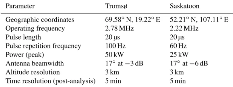
Full descriptions of the radar systems providing the un-derlying data used here are to be found in Hall (2001) and Manson and Meek (1991); the salient features of the radars relevant for this study are given in Table 1.
2 Analysis methodology
The characteristic fading time of the signal,τc, is used to
de-fine an indication of the upper limit for turbulent energy dis-sipation present in the atmosphere,ε′, as explained above. First, velocity fluctuations, v′, relative to the background wind are identified as
v′=λ
√
ln 2 4π τc
, (1)
whereλis the radar wavelength. This relationship has been presented and discussed by Briggs (1980) and Vandepeer and Hocking (1993). In turnv′2can be considered to represent the turbulent kinetic energy of the air such that the rate of dissipation of this energy is obtained by dividing by a charac-teristic timescale. If the Brunt–Väisälä periodTB(=2π/ωB
whereωBis the Brunt–Väisälä frequency in rad s−1)can be
Table 1.Salient radar parameters.
Parameter Tromsø Saskatoon
Geographic coordinates 69.58◦N, 19.22◦E 52.21◦N, 107.11◦E Operating frequency 2.78 MHz 2.22 MHz
Pulse length 20 µs 20 µs
Pulse repetition frequency 100 Hz 60 Hz
Power (peak) 50 kW 25 kW
Antenna beamwidth 17◦at−3 dB 17◦at−6 dB
Altitude resolution 3 km 3 km
Time resolution (post-analysis) 5 min 5 min
ε′=0.8v′2/TB, (2)
the factor 0.8 being related to an assumption of a total veloc-ity fluctuation (see Weinstock, 1978). Alternatively, this can be expressed as
ε′=0.8v′2ωB/2π, (3)
wherein the Brunt–Väisälä frequency is given by
ωB=
s
dT dz +
g cp
g
T, (4)
whereT is the neutral temperature,zis altitude,gis the ac-celeration due to gravity andcpis the specific heat of the air
at constant pressure. Due to viscosity, there is a minimum en-ergy dissipation rate, εmin, present in the atmosphere, given
by
εmin=ω2Bν/β, (5)
whereν is the kinematic viscosity. The factorβ, known as the mixing or flux coefficient (Oakey, 1982; Fukao et al., 1994; Pardyjak et al., 2002), is related to the flux Richard-son numberRf(β=Rf/(1−Rf)).Rfis in turn related to the
commonly used gradient Richardson number,Ri, by the ratio of the momentum to thermal turbulent diffusivities, or turbu-lent Prandtl number (e.g. Kundu, 1990). Fukao et al. (1994) proposed 0.3 as a value forβ. The relationships are fully de-scribed by Hall et al. (2008). The MF-radar system employed here to estimate turbulence is not well suited to estimatingRi
due to the height resolution of 3 km; moreover more detailed temperature information would be required to arrive atRf.
Anywhere in the atmosphere, energy dissipation is by the sum of the available processes. In this study, therefore, the turbulent energy dissipation rate can be considered the total rate minus that corresponding to viscosity:
ε=ε′−εmin. (6)
Importantly, the kinematic viscosity is given by the dynamic viscosity,µ, divided by the density,ρ:
ν=µ/ρ. (7)
Thus, since density is inversely proportional to temperature, kinematic viscosity is (approximately) linearly dependent on temperature;ω2Bis inversely proportional to temperature and thereforeεminis approximately independent of temperature.
On the other hand,ε′is proportional toωBand therefore
in-versely proportional to the square root of temperature. If we are able to estimate the energy dissipation rates de-scribed above, then the turbopause may be identified as the altitude at whichε=εmin. This corresponds to equality of
inertial and viscous effects and hence the condition where Reynolds number,Re, is unity as explained earlier.
To implement the above methodology, temperature data are required. Since observational temperature profiles can-not be obtained reliably, NRLMSISE-00 empirical model (Picone et al., 2002) profiles are, of necessity, used in the derivation of turbulent intensity from MF-radar data. The reasons for this are discussed in detail in the following sec-tion. While a temperature profile covering the UMLT region is not readily available by ground-based observations from Tromsø, meteor-trail echo fading times measured by the Nip-pon/Norway Tromsø Meteor Radar (NTMR) can be used to yield neutral temperatures at 90 km altitude. Any trend in temperature can usefully be obtained (the absolute values of the temperatures being superfluous since they are only available for one height). The method is exactly the same as used by Hall et al. (2012) to determine 90 km tempera-tures over Svalbard (78◦N) using a radar identical to NTMR. Hall et al. (2005) investigate the unsuitability of meteor radar data for temperature determination above∼95 km and below
∼85 km. In summary, ionisation trails from meteors are ob-served using a radar operating at a frequency less than the plasma frequency of the electron density in the trail (this is the so-called “underdense” condition). It is then possible to derive ambipolar diffusion coefficientsDfrom the radar echo decay times,τmeteor(as distinct from the corresponding
τmeteor= λ2
16π2D, (8)
wherein λis the radar wavelength. Thereafter the tempera-tureT may be derived using the relation
T = s
P·D 6.39×10⁻²K0
, (9)
whereP is the neutral pressure andK0is the zero field
mo-bility of the ions in the trail (here we assume K0=2.4×
10−4m−2s−1V−1)(McKinley, 1961; Chilson et al., 1996;
Cervera and Reid, 2000; Holdsworth et al., 2006). The pres-sure,P, was obtained from NRLMSISE-00 for consistency with the turbulence calculations. In the derivations by Dyr-land et al. (2010) and Hall et al. (2012), for example, temper-atures were then normalised to independent measurements by the MLS (Microwave Limb Sounder) on board the EOS (Earth Observing System) Aura spacecraft launched in 2004. The MLS measurements were chosen because the diurnal coverage was constant for all measurements, and it was there-fore simpler to estimate values that were representative of daily means than other sources such as SABER. In this way, the influence of any systematic deficiencies in NRLMSISE-00 (e.g. due to the age of the model) was minimised.
3 Results and implications for changing neutral air temperature
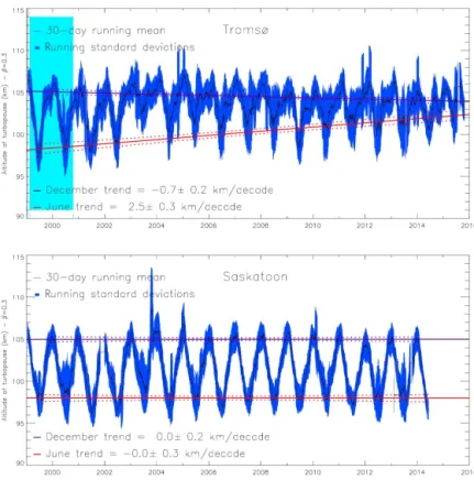
Following the method described above and by Hall et al. (1998b, 2008), the turbopause position is determined as shown in Fig. 1. The time and height resolutions of the MF radars used for the investigation are 5 min and 3 km respec-tively, and daily means of turbulent energy dissipation rate profiles are used to determine corresponding turbopause al-titudes. The figure shows the evolution since 1999: 70◦N, 19◦E (Tromsø) in the upper panel and 52◦N, 107◦W (Saska-toon) in the lower panel. Results are, of course, specific to these geographical locations and it must be stressed that they are in no way zonally representative (hereafter, though, “70◦N” and “52◦N” may be used to refer to the two lo-cations for convenience). Data are available from 1 Jan-uary 1999 to 25 June 2014 for Saskatoon, but thereafter tech-nical problems affected data quality. Data are shown from 1 January 1999 to 25 October 2015 for Tromsø. The cyan background corresponding to the period 16 February 1999 to 16 October 2000 in the 70◦N (Tromsø) panel indicates data available but using different experiment parameters, and thus 70◦N data prior to 17 October 2000 are excluded from this analysis. A 30-day running mean is shown by the thick lines with the shading either side indicating the standard deviation. The seasonal variation is clear to see, and for illustrative pur-poses, trend lines have been fitted to June and December val-ues together with hyperbolae showing the 95 % confidence
limits in the linear fits (Working and Hotelling, 1929); the seasonal dependence of the trends is addressed in more detail subsequently. The months of June and December are chosen simply because these correspond to the solstices and thus to avoid any a priori conception of when one could anticipate the maxima and minima to be. It is evident that, apart from the seasonal variation, the mid-latitude turbopause changes little over the period 1999–2014, whereas at high latitude there is more change for the summer state over the period 2001–2015 (the summers of 1999 and 2000 being excluded from the fitting due to changes in experiment parameters for the Tromsø radar). To investigate the seasonal dependence of the change further, the monthly values for 70 and 52◦N are shown in Fig. 2. Since 2001, the high-latitude turbopause has increased in height during late spring and mid-summer but otherwise remained constant. Since individual months are se-lected the possibility of “end-point” biases is not an issue in the trend-line fitting as would be the case if analysing en-tire data sets with non-integer numbers of years. Even so, certain years may be apparently anomalous, for example the summer of 2003. In this study, the philosophy is to look for any significant change in the atmosphere over the observa-tional period. If anomalous years are caused by, for example, changes in gravity-wave production (perhaps due to an in-creasing frequency of storm in the troposphere) and filtering in the underlying atmosphere, these too should be considered part of climate change. The trend (or overall change) over the observation period is indeed sensitive to exclusion of certain years. Although not illustrated here, this was tested briefly: selecting data from only 2004 onwards indicates no signif-icant change for summer, but a slightly increased negative winter change (to−1.7±0.2 K decade−1); excluding only
Figure 1.Turbopause altitude as determined by the definition and method described in this paper. The thick solid line shows the 30-day running mean and the shading behind it the corresponding standard deviations. The straight lines show the fits to summer and winter portions of the curve. Upper panel: 70◦N (Tromsø); lower panel: 52◦N (Saskatoon). The cyan background in the 70◦N panel indicates data available but unused here due to different experiment parameters.
radar because the geographical coverage of remote sensing data needs to be sufficiently large to obtain the required an-nual coverage, since the sampling region can vary with sea-son (depending on the satellite). Choice of the somewhat dated NRLMSISE-00 model at least allows the geographi-cal location to be specified and furthermore ensures a degree of consistency between the two sets of radar observations and also earlier analyses. The only ground-based temperature ob-servations both available and suitable are at 70◦N and 90 km altitude as described earlier and used subsequently.
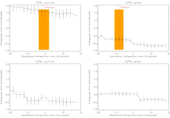
Next, we have attempted to investigate the effects of changing temperature. In a very simplistic approach, hy-pothetical altitude-invariant trends are imposed on the NRLMSISE-00 profiles. In other words, the same hypothet-ical trend is applied to all heights (in want of better infor-mation) in the NRLMSISE-00 profile to generate evolving (cooling or warming) temperature time series. The suggested trends vary from−20 to+20 K decade−1, thus well encom-passing any realistically conceivable temperature change (cf. Blum and Fricke, 2008; Danilov, 1997, Lübken, 1999). The result of applying hypothetical temperature trends to the time-invariant turbopause heights shown earlier is demon-strated in Fig. 3. Given the seasonal differences identified earlier, four combinations are shown: summer (average of May, June and July) and winter (average of November,
De-Figure 2.Trends for the period as a function of month. Upper panel: 70◦N (Tromsø); lower panel: 52◦N (Saskatoon).
cember and January) for each geographic location. Realis-tic temperature trends can be considered within the range
Figure 3.Response of turbopause trend line to different upper-mesosphere/lower-thermosphere temperature trends. Hypothetical trends range from an unrealistic cooling of 20 K decade−1to a similarly unrealistic warming. Top left: 70◦N summer (average of May, June and July); top right: 70◦N winter (average of November, December and January); bottom left: 52◦N summer; bottom right: 52◦N winter. Observed values for 70◦N are also identified on the upper panels (dashed vertical lines) together with uncertainties (shading).
In addition, the figure includes estimated trends obtained from observations, which shall be explained forthwith. The salient point arising from the figure is that no realistic tem-perature trend (at least given the simple model employed here) has the capability of reversing the corresponding trend in turbopause height.
In a recent study, Holmen et al. (2015) have built on the method of Hall et al. (2012) to determine 90 km tem-peratures over NTMR, as has been described in the pre-vious section. This new work presents more sophisticated approaches for normalisation to independent measurements and investigation of the dependence of derived tempera-tures on solar flux. Having removed seasonal and solar cy-cle variations in order to facilitate trend-line fitting (as op-posed to isolating a hypothetical anthropogenic-driven vari-ation), Holmen et al. (2015) arrive at a temperature trend of−3.6±1.1 K decade−1determined over the time interval 2004–2014 inclusive. This can be considered statistically sig-nificant (viz. sigsig-nificantly non-zero at the 5 % level) since the uncertainty (2σ=2.2 K decade−1)is less than the trend itself (e.g. Tiao et al., 1990).
Estimations of changes in temperature corresponding to the period for determination of the turbopause were only vi-able for 70◦N, these being−0.8±2.9 K decade−1for
sum-mer and−8.1±2.5 K decade−1for winter, and these results
are indicated in Fig. 3. Again the simple idea of superimpos-ing a gradual temperature change (the same for all heights)
on the temperature model used for the turbulence determina-tion thus fails to alter the change in turbopause height sig-nificantly, for the approximate decade of observations. Al-though direct temperature measurements are not available for the 52◦N site, Offermann et al. (2010) report cooling rates of ∼2.3 K decade−1for 51◦N, 7◦E, and She et al. (2015)
∼2.8 K decade−1for 42◦N, 112◦W. As for 70◦N, these re-sults do not alter the conclusions inferred from Fig. 3.
4 Discussion
tur-bopause, at least at mid-latitude (Oliver et al., 2014, and ref-erences therein). The rationale for this is that the atomic oxy-gen density [O] has been observed to increase during the time interval 1975–2014 at a rate of approximately 1 % year−1. The associated change in turbopause height may be estimated thusly as
H=RT /mg, (10)
where H is scale height, R is the universal gas con-stant (=8.314 J mol−1K−1),mis the mean molecular mass (kg mol−1) and g is the acceleration due to gravity. At 120 km altitude,gis taken to be 9.5 m s−2. For air and atomic oxygen,m=29 and 16 respectively. For a typical tempera-ture of 200 K, the two corresponding scale heights are there-fore Hair=6.04 km andHoxygen=10.94 km. If the change
(fall) in turbopause height is denoted by1hturb, then Oliver
et al. (2014) indicate that the factor by which [O] would in-crease is given by
exp(1hturb/Hair)/exp(1hturb/Hoxygen). (11)
Note that Oliver et al. (2014) state that “[O] . . . would in-crease by the amount”, but, since Eq. (1) is dimensionless, the reader should be aware this is a factor, not an absolute quantity. At first, there would appear to be a fundamental difference between the findings derived from [O] at a mid-latitude station and those for εfrom a high-latitude station, and indeed the paradox could be explained by either the re-spective methods and/or geographic locations. Usefully, in this context, Shinbori et al. (2014) and Kozubek et al. (2015) investigate such geographical diversity. However if one ex-amines the period from 2002 onwards (corresponding to the high-latitude data set, but only about one-quarter of that from the mid-latitude station), a decrease in [O] corresponds with an increase in1hturb. If1hturb for the measured
sum-mer temperature change at high latitude (viz. 0.16 km year−1 from Fig. 3) is inserted in Eq. (1) together with the suggested scale heights for air and atomic oxygen, one obtains a corre-sponding decrease in [O] of 16 % decade−1over the period 2002–2015. The corresponding time interval is not analysed per se by Oliver et al. (2014), but a visual inspection sug-gests a decrease of the order of 20 %; the decrease itself is incontrovertible and therefore in qualitative agreement with our high-latitude result.
It is somewhat unfortunate that it is difficult to locate si-multaneous and approximately co-located measurements by different methods. The turbopause height change by Oliver et al. (2014) is derived by measurements of [O] and at mid-latitude; those by Pokhunkov et al. (2009), also by exam-ining constituent scale heights, include determinations for Heiss Island (80◦N, 58◦E), but this rocket sounding pro-gramme was terminated prior to the start of our observation series (Danilov et al., 1979). It should be noted, however, that the results of seasonal variability presented by Danilov
et al. (1979) agree well with those described here giving cre-dence to the method and to the validity of the comparisons above.
background information, not only on the wind field but also on tidal amplitude perturbation due to deposition of gravity waves’ horizontal momentum.
5 Conclusion
Updated temporal evolutions of the turbopause altitude have been presented for two locations: 70◦N, 19◦E (Tromsø) and 52◦N, 107◦W (Saskatoon), the time interval now spanning 1999 to 2015. These turbopause altitude estimates are de-rived from estimates of turbulent energy dissipation rate ob-tained from medium-frequency radars. The method entails knowledge of neutral temperature that had earlier (Hall et al., 2008) been assumed to be constant with time. Here the response of the change in turbopause heights over the period of the study to temperature trends – both hypothetical and observed – is examined. No temperature trend scenario was capable of altering the observed turbopause characteristics significantly; at 70◦N, 19◦E an increase in turbopause height is evident during the 1999–2015 period for summer months, whereas for winter at 70◦N, 19◦E and all seasons at 52◦N, 107◦W the turbopause height has not changed significantly. In evaluating these results, however, there are a number of caveats that must be remembered. Firstly, the radar system does not perform well with an aurorally disturbed D region – the study, on the other hand incorporates well over 100 000 h of data for each radar site, and auroral conditions are occa-sional and of the order of a few hours each week at most. Secondly, an influence of the semi-empirical model used to provide both density and Brunt–Väisälä frequencies cannot be disregarded. It should also be stressed that a change is be-ing reported for the observational periods of approximately 15 years (i.e. just over one solar cycle) and parameterised by fitting linear trend lines to the data; this is distinct from asserting long-term trends in which solar and anthropogenic effects can be discriminated.
At first, this conclusion would appear to contradict the recent report by Oliver et al. (2014) and Pokhunkov et al. (2009). However, closer inspection shows that if one considers the time interval 2002–2012 in isolation, there is a qualitative agreement. In fact, we note that Oliver et al. (2014) deduce a turbopause change based on chang-ing atomic oxygen concentration and so we are similarly able to deduce a change in atomic oxygen concentration based on the change in turbopause height obtained from direct estimation of turbulence intensity. Given an average (i.e. not differentiating between seasons) temperature change of −3.4±0.5 K decade−1 for 70◦N, 19◦E (Tromsø), the change in turbopause height in summer over the same time interval is 1.6±0.3 km decade−1 suggesting a decrease in atomic oxygen concentration of 16 %.
The primary aim of this study is to demonstrate the in-creasing altitude of the summer turbopause at 70◦N, 19◦E and the apparently unvarying altitude in winter and at 52◦N,
107◦W during the time interval 1999–2014. Independent studies using a radically different method demonstrate how to infer a corresponding decrease in atomic oxygen concen-tration, as a spin-off result. Finally, the question as to the exact mechanism causing the evolution of turbulence in the lower thermosphere at, in particular 70◦N, 19◦E, remains unanswered. Furthermore, dynamics at this particular geo-graphic location may be pathological. The solution perhaps lies in seasonally dependent gravity wave filtering in the un-derlying atmosphere being affected by climatic tropospheric warming and/or middle atmosphere cooling; hitherto, how-ever, this remains a hypothesis.
Acknowledgements. The authors thank the referees of this paper.
Edited by: G. Stiller
References
Batchelor, G. K.: The theory of homogeneous turbulence, 197 pp., Athenaceum Press Ltd., Newcastle-upon-Tyne, Great Britain, 1953.
Blum, U. and Fricke, K. H.: Indications for a long-term temperature change in the polar summer middle atmosphere, J. Atmos. Sol.-Terr. Phy., 70, 123–137, 2008
Briggs, B. H.: Radar observations of atmospheric winds and tur-bulence: a comparison of techniques, J. Atmos. Terr. Phys., 42, 823–833, 1980.
Cervera, M. A. and Reid, I. M.: Comparison of atmospheric param-eters derived from meteor observations with CIRA, Radio Sci., 35, 833–843, 2000.
Chilson, P. B., Czechowsky, P., and Schmidt, G.: A comparison of ambipolar diffusion coefficients in meteor trains using VHF radar and UV lidar, Geophys. Res. Lett., 23, 2745–2748, 1996. Cnossen, I., Laštoviˇcka, J., and Emmert, J. T.: Introduction to
spe-cial issue on “Long-term changes and trends in the stratosphere, mesosphere, thermosphere and ionosphere”, J. Geophys. Res., 120, 11401–11403, doi:10.1002/2015JD024133, 2015.
Cullens, C. Y., England, S. L., and Immel, T. J.: Global responses of gravity waves to planetary waves during stratospheric sudden warming observed by SABER, J. Geophys. Res., 120, 12018– 12026, doi:10.1002/2015JD023966, 2015.
Danilov, A. D., Kalgin, U. A., and Pokhunov, A. A.: Variation of the mesopause level in polar regions, Space Res. XIX, 83, 173–176, 1979.
Dyrland, M. E., Hall, C. M., Mulligan, F. J., and Tsutsumi, M.: Im-proved estimates for neutral air temperatures at 90 km and 78◦N using satellite and meteor radar data, Radio Sci., 45, RS4006, doi:10.1029/2009RS004344, 2010.
Fu, Q., Lin, P., Solomon, S., and Hartmann, D. L.: Observa-tional evidence of the strengthening of the Brewer-Dobson circulation since 1980, J. Geophys. Res., 120, 10214–10228, doi:10.1002/2015JD023657, 2015.
1. Three-year observations by the middle and upper atmosphere radar, J. Geophys. Res., 99, 18973–18987, 1994.
Hall, C. M.: The Ramfjormoen MF radar (69◦N, 19◦E): Applica-tion development 1990–2000, J. Atmos. Sol.-Terr. Phy., 63, 171– 179, 2001.
Hall, C. M.: The radar tropopause above Svalbard 2008–2012: char-acteristics at various timescales, J. Geophys. Res., 118, 2600-2608, doi:10.1002/jgrd.50247, 2013.
Hall, C. M., Blix, T. A., Thrane, E. V., and Lübken, F.-J.: Sea-sonal variation of mesospheric turbulent kinetic energy dissipa-tion rates at 69◦N, Proc. 13th ESA symposium, 505–509, 1997. Hall, C. M., Manson, A. H., and Meek, C. E.: Measurements of the
arctic turbopause, Ann. Geophys., 16, 342–345, 1998a. Hall, C. M., Manson, A. H., and Meek, C. E.: Seasonal variation of
the turbopause: One year of turbulence investigation at 69◦N by the joint University of Tromsø/University of Saskatchewan MF radar, J. Geophys. Res., 103, 28769–28773, 1998b.
Hall, C. M., Aso, T., Tsutsumi, M., Nozawa, S., Manson, A. H., and Meek, C. E.:Letter to the EditiorTesting the hypothesis of the influence of neutral turbulence on the deduction of ambipo-lar diffusivities from meteor trail expansion, Ann. Geophys., 23, 1071–1073, doi:10.5194/angeo-23-1071-2005, 2005.
Hall, C. M., Meek, C. E., Manson, A. H., and Nozawa, S.: Tur-bopause determination, climatology and climatic trends, using medium frequency radars at 52◦ and 70◦N, J. Geophys. Res., 113, D13104, doi:10.1029/2008JD009938, 2008.
Hall, C. M., Dyrland, M. E., Tsutsumi, M., and Mulligan, F.: Temperature trends at 90 km over Svalbard seen in one decade of meteor radar observations, J. Geophys. Res., 117, D08104, doi:10.1029/2011JD017028, 2012.
Hocking, W. K.: On the extraction of atmospheric turbulence pa-rameters from radar backscatter Doppler spectra – I. Theory, J. Atmos. Terr. Phys., 45, 89–102, 1983.
Hocking, W. K.: An assessment of the capabilities and limitations of radars in measurements of upper atmosphere turbulence, Adv. Space Res., 17, 37–47, 1996.
Hoffmann, P., Rapp, M., Singer, W., and Keuer, D.: Trends of mesospheric gravity waves at northern middle lati-tudes during summer, J. Geophys. Res., 116, D00P08, doi:10.1029/2011JD015717, 2011.
Holdsworth, D. A., Morris, R. J., Murphy, D. J., Reid, I. M., Burns, G. B., and French, W. J. R.: Antarctic mesospheric temperature estimation using the Davis MST radar, J. Geophys. Res., 111, D05108, doi:10.1029/2005JD006589, 2006.
Holmen, S. E., Hall, C. M., and Tsutsumi, M.: Neutral atmosphere temperature change at 90 km, 70◦N, 19◦E, 2003–2014, Atmos. Chem. Phys. Discuss., 15, 15289–15317, doi:10.5194/acpd-15-15289-2015, 2015.
Jackman, C. H., DeLand, M. T., Labow, G. J., Fleming, E. L., Weisenstein, D. K., Ko, M. K. W., Sinnhuber, M., Anderson, J., and Russel, J. M.: The influence of the several very large so-lar proton events in years 2000–2003 on the middle atmosphere, Adv. Space Res., 35, 445–450, doi:10.1016/j.asr.2004.09.006, 2005.
Kolmogorov, A. N.: Dissipation of energy in the locally isotropic turbulence, Proc. USSR Academy of Sciences, 30, 299–303, 1941.
Kozubek, M., Krizan, P., and Lastovicka, J.: Northern Hemisphere stratospheric winds in higher midlatitudes: longitudinal
distribu-tion and long-term trends, Atmos. Chem. Phys., 15, 2203–2213, doi:10.5194/acp-15-2203-2015, 2015.
Krivolutsky, A. A., Klyuchnikova, A. V., Zakharov, G. R., Vyushkova, Y. T., and Kuminov, A. A.: Dynamical response of the middle atmosphere to solar proton event of July 2000: three dimensional model simulations, Adv. Space Res., 37, 1602– 1613, doi:10.1016/j.asr.2005.05.115, 2006.
Kundu, P. K.: Fluid Mechanics, 638 pp., Academic Press, San Diego, USA, 1990.
Lübken, F.-J.: Nearly zero temperature trend in the polar summer mesosphere, Geophys. Res. Lett., 104, 9135–9149, 1999. Manson, A. H. and Meek, C. E.: Climatologies of mean winds and
tides observed by medium frequency radars at Tromsø (70N) and Saskatchewan (52N) during 1987–1989, Can. J. Phys., 69, 966– 975, 1991.
Manson, A. H., Meek, C. E., Xu, X., Aso, T., Drummond, J. R., Hall, C. M., Hocking, W. K., Tsutsumi, M., and Ward, W. E.: Characteristics of Arctic winds at CANDAC-PEARL (80◦N, 86◦W) and Svalbard (78◦N, 16◦E) for 2006–2009: radar observations and comparisons with the model CMAM-DAS, Ann. Geophys., 29, 1927–1938, doi:10.5194/angeo-29-1927-2011, 2011.
McIntyre, M. E.: On dynamics and transport near the polar mesopause in summer, J. Geophys. Res., 94, 20841–20857, 1991.
McKinley, D. W. R.: Meteor Science and Engineering, 309 pp., McGrath-Hill, New York, 1961.
Oakey, N. S.: Determination of the rate of dissipation of turbu-lent energy from simultaneous temperature and velocity shear microstructure measurements, J. Phys. Oceanogr., 12, 256–271, 1982.
Offermann, D., Jarisch, M., Schmidt, H., Oberheide, J., Grossmann, K. U., Gusev, O., Russell III, J. M., and Mlynczak, M. G.: The “wave turbopause”, J. Atmos. Sol.-Terr. Phy., 69, 2139–2158, 2007.
Offermann, D., Hoffmann, P., Knieling, P., Koppmann, R., Ober-heide, J., and Steinbrecht, W.: Long-term trends and solar cy-cle variations of mesospheric temperature and dynamics, J. Geo-phys. Res., 115, D18127, doi:10.1029/2009JD013363, 2010. Oliver, W. L., Holt, J. M., Zhang, S.-R., and Goncharenko, L. P.:
Long-term trends in thermospheric neutral temperature and den-sity above Millstone Hill, J. Geophys. Res.-Space, 119, 1–7, doi:10.1002/2014JA020311, 2014.
Pardyjak, E. R., Monti, P., and Fernando, H. J. S.: Flux Richardson number measurements in stable atmospheric shear flows, J. Fluid Mech., 459, 307–316, doi:10.1017/S0022112002008406, 2002. Picone, J. M., Hedin, A. E., Drob, D. P., and Atkin, A. C.:
NRLMSISE-00 empirical model of the atmosphere: statistical comparisons and scientific issues, J. Geophys. Res., 107, 1468, doi:10.1029/2002JA009430, 2002.
Pokhunkov, A. A., Rybin, V. V., and Tulinov, G. F.: Quantitative characteristics of long-term changes in parameter of the upper at-mosphere of the Earth over the 1966–1992 period, Cosmic Res., 47, 480–490, 2009
Schlegel, K., Brekke, A., and Haug, A.: Some characteristics of the quiet polar D-region and mesosphere obtained with the partial reflection method, J. Atmos. Terr. Phys., 40, 205–213, 1978. She, C.-Y., Krueger, D. A., and Yuan, T.: Long-term midlatitude
cen-tury (1990–2014) Na lidar observations, Ann. Geophys., 33, 363–369, doi:10.5194/angeo-33-363-2015, 2015.
Shinbori, A., Koyama, Y., Nose, M., Hori, T., Otsuka, Y., and Yata-gai, A.: Long-term variation in the upper atmosphere as seen in the geomagnetic solar quiet daily variation, Earth Planet. Space, 66, 155–175, doi:10.1186/s40623-014-0155-1, 2014.
Stray, N. H., Orsolini, Y. J., Espy, P. J., Limpasuvan, V., and Hib-bins, R. E.: Observations of planetary waves in the mesosphere-lower thermosphere during stratospheric warming events, At-mos. Chem. Phys., 15, 4997–5005, doi:10.5194/acp-15-4997-2015, 2015.
Tiao, G. C., Reinsel, G. C., Xu, D., Pedrick, J. H., Zhu, X., Miller, A. J., DeLuisi, J. J., Mateer, C. L., and Wuebbles, D. J.: Effects of autocorrelation and temporal sampling schemes on estimates of trend and spatial correlation, J. Geophys. Res., 95, 20507–20517, 1990.
Thrane, E. V., Blix, T. A., Hall, C., Hansen, T. L., von Zahn, U., Meyer, W., Czechowsky, P., Schmidt, G., Widdel, H.-U., and Neumann, A.: Small scale structure and turbulence in the meso-sphere and lower thermomeso-sphere at high latitudes in winter, J. At-mos. Terr. Phys., 49, 751–762, 1987.
Vandepeer, B. G. W. and Hocking, W. K.: A comparison of Doppler and spaced antenna radar techniques for the measurement of tur-bulent energy dissipation rates, Geophys. Res. Lett., 20, 17–20, 1993.
Weinstock, J.: Vertical turbulent diffusion in a stably stratified fluid, J. Atmos. Sci., 35, 1022–1027, 1978.
de Wit, R. J., Hibbins, R. E., Espy, P. J., and Hennum, E. A.: Coupling in the middle atmosphere related to the 2013 ma-jor sudden stratospheric warming, Ann. Geophys., 33, 309–319, doi:10.5194/angeo-33-309-2015, 2015.