www.hydrol-earth-syst-sci.net/14/251/2010/ © Author(s) 2010. This work is distributed under the Creative Commons Attribution 3.0 License.
Earth System
Sciences
Uncertainty in the determination of soil hydraulic parameters and
its influence on the performance of two hydrological models of
different complexity
G. Baroni1, A. Facchi1, C. Gandolfi1, B. Ortuani1, D. Horeschi2, and J. C. van Dam3
1Dipartimento di Ingegneria Agraria, Universit`a degli Studi di Milano, Italy
2Dipartimento di Ingegneria Idraulica, Ambientale, delle Infrastrutture Viarie e del Rilevamento, Politecnico di Milano, Italy 3Department of Environmental Sciences, Wageningen University, The Netherlands
Received: 12 May 2009 – Published in Hydrol. Earth Syst. Sci. Discuss.: 4 June 2009 Revised: 26 January 2010 – Accepted: 27 January 2010 – Published: 9 February 2010
Abstract. Data of soil hydraulic properties forms often a limiting factor in unsaturated zone modelling, especially at the larger scales. Investigations for the hydraulic character-ization of soils are time-consuming and costly, and the ac-curacy of the results obtained by the different methodologies is still debated. However, we may wonder how the uncer-tainty in soil hydraulic parameters relates to the unceruncer-tainty of the selected modelling approach. We performed an inten-sive monitoring study during the cropping season of a 10 ha maize field in Northern Italy. The data were used to: i) com-pare different methods for determining soil hydraulic param-eters and ii) evaluate the effect of the uncertainty in these pa-rameters on different variables (i.e. evapotranspiration, aver-age water content in the root zone, flux at the bottom bound-ary of the root zone) simulated by two hydrological models of different complexity: SWAP, a widely used model of soil moisture dynamics in unsaturated soils based on Richards equation, and ALHyMUS, a conceptual model of the same dynamics based on a reservoir cascade scheme. We em-ployed five direct and indirect methods to determine soil hy-draulic parameters for each horizon of the experimental pro-file. Two methods were based on a parameter optimization of: a) laboratory measured retention and hydraulic conduc-tivity data and b) field measured retention and hydraulic con-ductivity data. The remaining three methods were based on the application of widely used Pedo-Transfer Functions: c) Rawls and Brakensiek, d) HYPRES, and e) ROSETTA. Sim-ulations were performed using meteorological, irrigation and crop data measured at the experimental site during the pe-riod June – October 2006. Results showed a wide range of soil hydraulic parameter values generated with the different
Correspondence to:G. Baroni ([email protected])
methods, especially for the saturated hydraulic conductivity Ksatand the shape parameterαof the van Genuchten curve.
This is reflected in a variability of the modeling results which is, as expected, different for each model and each variable analysed. The variability of the simulated water content in the root zone and of the bottom flux for different soil hy-draulic parameter sets is found to be often larger than the difference between modeling results of the two models using the same soil hydraulic parameter set. Also we found that a good agreement in simulated soil moisture patterns may occur even if evapotranspiration and percolation fluxes are significantly different. Therefore multiple output variables should be considered to test the performances of methods and models.
1 Introduction
Water retention and hydraulic conductivity curves are crucial input data in any modelling study on water flow and solute transport. Computed water balances are very sensitive to soil hydraulic parameters and therefore their accurate determina-tion is essential to model hydrological processes (Jhorar et al., 2004). Moreover, at most sites soil hydraulic parame-ters are characterized by a strong variability in both vertical and horizontal directions. Therefore a large number of data are required to properly describe the hydraulic properties of an area.
The first techniques rely on precise experimental proce-dures that can be categorized as being either laboratory- or field-based. Laboratory methods are based on the accurate measurement of flow processes, but they are generally per-formed on small soil samples and as a result their represen-tativeness of field conditions can be questioned. In addition, the presence of stones, fissures, fractures, tension cracks, root holes, as commonly encountered in unsaturated soil profiles, is difficult to be captured in small-scale laboratory samples. Field techniques can be more difficult to manage and con-trol, but they offer the possibility to directly measure more representative soil hydraulic properties.
However, despite the progress that has been achieved, the measurement techniques remain time consuming and costly, especially when data are needed for large areas (W¨osten et al., 2001). For this reason the definition of reliable meth-ods for estimating soil hydraulic properties in areas where the amount of available information is limited remains a key issue. This explains why many attempts have been made at estimating soil hydraulic parameters by means of empir-ical relationships based on readily available soil data, such as textural soil properties and bulk density. These relation-ships, commonly referred as Pedo Transfer Functions (PTFs) (Bouma and van Lanen, 1987; Bouma, 1989), are particu-larly enticing as they are very well suited for large scale ap-plications.
In general these relationships are based on statistical re-gression (e.g. Gupta and Larson, 1979; Rawls and Brak-ensiek, 1989; Cosby et al., 1984; Vereecken et al., 1989; W¨osten et al., 1999; Saxton and Rawls, 2006), although some authors tried to develop more physically-based re-lationships (e.g. D’Urso and Basile, 1997). Some au-thors developed different approaches, like artificial neural networks (Minasny and McBratney, 2002; Schaap et al., 2001) or group methods of data handling (Pachepsky and Rawls, 1999), and promising results were obtained lately with support vector machines (Navin et al., 2009; Lamorski et al., 2008) and non-parametric pattern recognition tools (e.g. Nemes et al., 2006b, c). One of the advantage with these last methods is that the identification of an a priori relation between input and output data is not needed.
In spite of the wide application of these methodologies, the reliability of the results obtained is still under discussion (e.g. Tietje and Hennings, 1996; Romano, 1999). In most cases the methods are evaluated by comparing the values of selected soil hydraulic parameters obtained by the measure-ment techniques that are supposed to be more accurate with the indirectly estimated parameter values (Tietje and Tapken-hinrichs, 1993; Bastet et al., 1999; Nemes et al., 2003; Un-garo et al., 2005). These comparisons show that good perfor-mances can be obtained with predictive methods, but gener-ally the results are site-specific. Therefore it is not possible to draw general conclusions about which methods are the best for a certain modeling purpose.
results were shown by Christiaens and Feyen (2001). Guber et al. (2009) showed that good performances for soil water content can be obtained considering several PTFs (i.e. in their case 19) and using appropriate methods (i.e. equal weights, Bayesian model averaging, etc.) to combine the water mois-ture patterns predicted by using a Richards equation-based model with the different PTFs .
Workmann and Skaggs (1994) used two hydrological models of different complexity considering the uncertainty in the soil hydraulic parameter sets. Results pointed out that for the case study the model concept uncertainty was less impor-tant than parameters uncertainty. These findings motivate to further investigate under what circumstances the differences among modeling schemes are overwhelmed by uncertainty in the soil hydraulic parameters.
In spite of the large number of existing hydrological mod-els, there are only two main approaches used for the mathe-matical representation of water flow in the unsaturated zone: numerical solutions of the Richards equation and reservoir cascade schemes. The Richards equation is the fundamen-tal governing equation for the description of the flow in un-saturated porous media. Models based on its numerical so-lution were at first developed for the local scale and gener-ally applied after a detailed calibration. Examples are SOIL (Johnson and Jansson, 1991), SWAP (van Dam et al., 1997), HYDRUS (Simunek et al., 1998). Nowadays, a number of physically based distributed-parameters models have become available, such as HydroGeoSphere (Sudicky et al., 2006), LGM-SWAP (Stoppelenburg et al., 2005), WaSiM (Schulla and Jasper, 2001), MIKE-SHE (Refsgaard and Storm, 1995). On the other hand, reservoir schemes have been adopted for decades in many hydrological models across scales, from field to global: EPIC (Sharpley and Williams, 1990), WEPP (Flanagan and Livingston, 1995), ANSWERS-2000 (Bouraoui and Dillaha, 1996), SWAT (Neitsch et al., 2002), UZF1 (Niswonger et al., 2006) are just few of the existing models. Due to the simplifications in the representation of the system, which very often makes them more comprehen-sible and manageable to non-expert final users, conceptual models are computationally efficient and stable. For these reasons they are still very attractive in many practical appli-cations, such as large scale simulations, for which usually long time periods are considered and repeated simulations are required (e.g. scenario analysis).
To what extent, or under what conditions, the simpler reservoir models can capture the main features of water trans-fer dynamics in the unsaturated zone, at the local or at larger scales, is still an open question. A number of studies on mod-els intercomparison have been conducted (e.g. Herbst et al., 2005; Eitzinger et al., 2004; Guswa et al., 2002; Maraux et al., 1998; Workmann and Skaggs, 1994), but rarely the effect of the uncertainty in model parameters or inputs has been taken into account in the analysis.
In order to further explore all these issues, in this study data collected in an intensive monitoring campaign were used to: i) compare five direct and indirect methods for de-riving the values of soil hydraulic parameters and ii) evalu-ate the effect of the uncertainty in the determination of these parameters with respect to the resulting uncertainty in the outputs of two hydrological models of different complexity: SWAP (Kroes and van Dam, 2003) based on the numerical solution of the Richards equation, and ALHyMUS (Facchi et al., 2004; Gandolfi et al., 2006) based on a reservoir cas-cade scheme. Simulations were run for each model and each parameter set using inputs and crop parameters measured in a 10 ha maize field. Daily values of evapotranspiration, av-erage soil water content in the root zone and water flux at the root zone bottom monitored in the field were used to test the performances of the methods to determine soil hydraulic parameters when used in the two hydrological models.
2 Materials and methods
2.1 Experimental field site
The monitoring activities were conducted during the crop-ping season 2006 in a 10 ha maize field located in Northern Italy (Landriano – PV), in the experimental farm A. Menozzi of the Agricultural Faculty of the State University of Milan (45◦19′N, 9◦15′E, 88 m a.s.l.).
Instruments for detailed monitoring of water and energy fluxes were installed in the experimental field in 2005. A mi-crometeorological eddy-covariance (EC) based station was located in the centre of the field. The station was equipped with: a 4-component radiometer (Kipp & Zonen CNR-1), an infrared gas analyzer (LI-COR 7500) and a 3D sonic anemometer (Young RM-81000V). Soil heat flux monitor-ing by means of heat flux plates (Hukseflux HFP01) and soil thermocouples (ELSI) allowed to close the surface energy balance.
Table 1.Summary of the main data collected at the monitoring site (3 June–10 October 2006).
Cumulative rain 429 mm
Mean temperature 21◦C
Crop Zea Mays
Emergence 6 June 2006 (DoY=157)
Harvesting 10 October 2006 (DoY=283)
LAImax 4.2
Crop heightmax 3.00 m
Rooting depthmax 0.70 m
Sprinkler irrigation event 8 June 2006 (DoY=159); 20 mm Surface irrigation event 14 July 2006 (DoY=195); 140 mm
Water table depth 0.90–1.20 m
Spatially distributed measurements of leaf area index LAI (–), crop heighthc(m), and rooting depthDr (m), were
conducted periodically to characterize the crop in the field. Moreover, saturated hydraulic conductivity Ksat (cm h−1)
was determined at depths of 20, 35 and 70 cm by means of a Guelph permeameter.
During the cropping season 2006 there were two irrigation treatments: the first one on 8 June (DoY=159) with the sprin-kler method to promote crop emergence, and the second one on 14 July (DoY=195) with the border method. The gross amount of water applied by the hose-raingun system during the first irrigation was controlled as carefully as possible dur-ing the operations, resultdur-ing in an average irrigation depth of 25 mm. In order to confirm this amount, the measurements of the soil moisture sensors installed at different depths were used to derive the increase in soil moisture stocked in the profile after the irrigation. Only the values measured by the three upper probes showed significant changes and gave an estimated 20 mm increase in soil moisture. Taking into ac-count the water losses before reaching the soil surface this value is in good agreement with the gross irrigation amount and it was therefore considered as the net irrigation supply at the soil surface.
At the second irrigation, the canal water discharge was monitored by an electromagnetic flow sensor (Nautilus -OTT), yielding an irrigation amount of 140 mm. The run-off was negligible in the entire monitoring period.
A summary of the main data collected at the monitoring site is shown in Table 1. Texture and organic matter mea-surements for the horizons identified in the soil profile are reported in Table 2.
2.2 SWAP model
The soil-water-atmosphere-plant (SWAP) model is a widely applied and well documented model, based on a finite dif-ference solution of the Richards equation (van Dam et al., 1997). It simulates the vertical soil water flow and solute transport in close interaction with crop growth. Richards
Table 2.Chemical-physical data for the horizons of the experimen-tal soil profile.
Depth (cm) 0–10 10–40 40–55 55–90
Horizons (USDA system) Ap1 Ap2 B 2Bt1
Sand (%) 67.0 65.0 56.0 44.5
Silt (%) 30.5 32.0 39.5 31.5
Clay (%) 2.5 3.0 4.5 24.0
Organic matter (%) 2.7 2.3 1.9 0.5
Bulk density (g cm−3) 1.19 1.24 1.30 1.60
equation (Richards, 1931) is applied to compute transient soil water flow:
C (h)∂h ∂t =
∂ ∂z
K (h)
∂h
∂z+1
−Sa (1)
where C(h) (cm−1) is the differential soil water capacity
(∂θ/∂h),θ(–) is the volumetric water content,h(cm) the soil water pressure head,K(h)(cm d−1)the hydraulic conductiv-ity,Sa(d−1)the root water extraction rate, andz(cm) the
ver-tical coordinate (positive upward). The numerical solution of Eq. (1) is subjected to specified initial and boundary condi-tions, and requires known relationships between the soil hy-draulic variables moistureθ, pressure head hand hydraulic conductivityK. The following relations between these vari-ables were used (van Genuchten, 1980; Mualem, 1976): θ (h)=θr+
θs−θr
1+ |αh|nm (2)
K (θ )=KsatSeL
1−
1−S 1
m e
m2
(3) whereθr (–) is the residual water content,θs(–) the saturated
water content, Se=(θ−θr)/(θs−θr)(–) the relative
satura-tion,α(cm−1),n(–), andmare empirical shape factors,Ksat
(cm h−1)the saturated hydraulic conductivity, andL(–) an
empirical coefficient. The value ofmis fixed asm=1−1/n. Canopy interception is calculated according to Braden (1985) as a function of the leaf area index (LAI). SWAP includes both a simple and detailed crop growth module. We used the simple crop module, in which crop growth is prescribed by LAI, crop height and rooting depth as functions of crop development stage. The potential evapotranspiration rate ETp (mm d−1) is estimated by the
Penman–Monteith equation (Monteith, 1965; Allen et al., 1998). In field conditions where crops partly cover the soil, ETp is partitioned into the potential soil evaporation Ep
(mm d−1)and the potential crop transpirationTp (mm d−1)
2.3 ALHyMUS model
The soil water model ALHyMUS (Facchi et al., 2004; Gan-dolfi et al., 2006) is based on a non-linear reservoir cascade scheme, including two reservoirs in the root-zone and one (or more) additional reservoir(s) extending from the root-zone to the groundwater table. The first reservoir represents the upper part of the soil profile in which infiltration, evapora-tion and percolaevapora-tion to the subsequent reservoir take place. The second reservoir extends through the root zone having a thickness variable with the phenology of the crop and con-siders the processes of transpiration and percolation to the reservoir beneath; in the last reservoir(s) only percolation is taken into account. The thickness of the last reservoir(s) may vary in time, depending on the fluctuations of phreatic levels. Canopy interception is evaluated by the Braden formula (Braden, 1985). Evaporative and transpirative rates are computed using the FAO-56 dual crop coefficient method (Allen et al., 1998). A one-dimensional mathematical rep-resentation of the infiltration and percolation processes is adopted: the potential infiltration rate is estimated by the Green-Ampt equation (Green and Ampt, 1911); drainage dis-charges from each reservoir are determined using a simpli-fied scheme, similar to those used in other conceptual models (e.g. ANSWERS-2000, Bouraoui and Dillaha, 1996; EPIC, Sharpley and Williams, 1990), which considers a Darcian-type gravity flow; the relationship between the unsaturated hydraulic conductivity and the water content is modelled by Eq. (3). The influence of a shallow groundwater table is ac-counted for by the formula proposed by Liu et al. (2006), which gives the capillary riseGc(mm d−1)from the
ground-water surface to the transpirative reservoir as a function of the water content in the reservoirθv(–), the rate of potential
evapotranspiration ETp(mm d−1)and the groundwater depth D(cm). Finally, all these terms are included in the daily wa-ter balance equations of the reservoirs, which are solved by an implicit iterative procedure.
2.4 Soil hydraulic parameters
Five different methods were used to estimate the soil hy-draulic parametersθs,θr,α, n,L andKsat: parameter
op-timisation of retention and hydraulic conductivity data mea-sured both in the laboratory and in the field, and three well-known Pedo-Transfer Functions applied to commonly avail-able field measurements of chemical-physical soil proper-ties: Rawls and Brakensiek (1989), HYPRES (W¨osten et al., 1999), ROSETTA (Schaap et al., 2001). The methods are coded in the text as LAB, f, RB, H and Ro respectively. 2.4.1 Laboratory measurements
Laboratory measurements were performed on undisturbed soil cores with diameterd=7.5 cm and heighth=5 cm taken in replicate from each of the four soil horizons (total of eight cores). The samples were collected before tillage and related
management activities took place on the bare soil. For each soil core, saturated hydraulic conductivity Ksat (cm h−1)
was determined by the standard constant head technique (Reynolds et al., 2002). Soil water contents were measured for 13 matric pressure heads allowing drainage water reten-tion characteristics to be determined from saturareten-tion to about
−300 cm using suction tables as described by Romano et al. (2002). Three additional points of the water retention function were measured with the pressure chamber method (corresponding to matric pressure head values of −3000,
−6000 and −12 000 cm). The water retention function of van Genuchten (1980) was fitted to the measuredθ−h val-ues using the RETC code (van Genuchten et al., 1991). In the optimisation,θsvalues were fixed to those determined in the
laboratory. The unsaturated hydraulic conductivity relation-ship was determined by using the water retention parameters plus the measured saturated hydraulic conductivity, accord-ing to the Mualem-van Genuchten model (van Genuchten, 1980).
2.4.2 Field measurements
Simultaneous field measurements of soil water content by soil moisture sensors and pressure head by tensiometers were collected in the experimental site at the depths of 20, 35 and 70 cm during the monitoring period June–October 2006. The water retention function of van Genuchten (1980) was fitted to the field measured θ−h values using the RETC code (van Genuchten et al., 1991). In the optimisation, θs
values were fixed to those determined during the calibra-tion of the CS probes, conducted in laboratory on samples collected in the summer 2006, after tillage activities. Satu-rated hydraulic conductivityKsat(cm h−1)was measured by
a Guelph permeameter at the same depths as the monitored θ−hvalues. As in the case of the laboratory measurements, the unsaturated hydraulic conductivity relationship was de-termined by using the water retention parameters plus the saturated hydraulic conductivity, according to the Mualem-van Genuchten model (Mualem-van Genuchten, 1980).
No field measurements of pressure head were available for the 1st (0–10 cm) and the 3rd (40–55 cm) horizon of the soil profile (see Table 2). Due to this lack of data, we had to assume that the soil hydraulic parameters obtained by the measurements taken at 20 cm and 70 cm depth were repre-sentative of the 1st and the 3rd horizon, respectively. This assumption shall be kept in mind when looking at the sim-ulation results because, while the properties of the first two horizons are rather similar, there is a change to a more clayey texture at 55 cm depth (Table 2).
(3 June 2006; DoY=154) to allow the mechanical operations to be carried out uniformly in the whole field. After this date the instruments were re-installed. The Guelph permeameter measurements of saturated hydraulic conductivity were also carried out during the cropping season.
2.4.3 Pedo-Transfer functions
Three widely used Pedo-Transfer Functions were applied to the texture and organic matter measurements available for the experimental profile (Table 2). The first one is the PTF of Rawls and Braekensiek (1989), based on non-linear multiple regression equations. Ungaro and Calzolari (2001) showed that these PTFs, even if based on US soils data base, have a good performance also for soils of the central Padana Plain (Northern Italy). The second PTF used is the so-called HYPRES (W¨osten et al., 1999), derived by multiple regres-sion techniques as well, but using a European data base of soils (although no soils of Northern Italy are included). The third PTF set used is ROSETTA (Schaap et al., 2001), devel-oped by the United States Salinity Laboratory using a neural network, and based on US soil data.
The bulk densityρb (g cm−3)used in the PTFs was
es-timated from the organic matter OM (%) values (Table 2) by the relationship proposed by Jeffrey et al. (1970), which showed to provide good results for the soils data of the area (ERSAL, 2001).
2.5 Model inputs and parameters
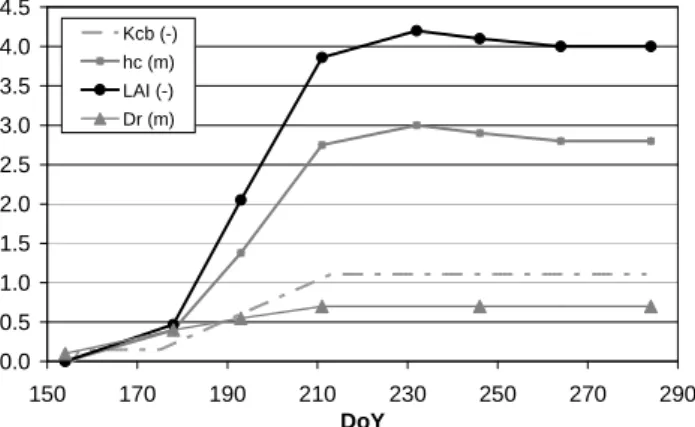
The models were run with the different sets of soil parame-ters for the period 6 June–10 October 2006 (DoY=157–283). Measured meteorological and irrigation data were used for the simulations. Daily values of crop height hc (m), leaf
area index LAI (–) and rooting depthDr (m) were obtained
by linear interpolation of the field data collected during the cropping season (Fig. 1). The daily pattern of basal crop co-efficientKcb(–) (Allen et al., 1998), used by ALHyMUS to
compute the transpiration rateTp (cm d−1), was estimated
on the basis of literature values (Allen et al., 1998; Huygen et al., 1997; Borgarello et al., 1993) and adapted to the crop-ping stages observed in the field (Fig. 1). Table 3 shows the additional crop parameters needed for the implementation of the two models. Pressure head valuesHLim1–HLim5(cm) for
crop water stress conditions in SWAP are those proposed for maize in Hupet et al. (2004). The canopy resistance rc(s m−1)for the SWAP Penman–Monteith equation is that
proposed in literature for maize (Kroes and van Dam, 2003). Literature values were also adopted fork(–), the extinction coefficient for global solar radiation, anda(mm d−1), an em-piric parameter used in the interception equation (Braden, 1985). The value of p (–), used by ALHyMUS to deter-mine the fraction of Readily Avalilable Water (RAW) from the Total Available Water (TAW), is that proposed in Allen et al. (1998) for maize.
0.0 0.5 1.0 1.5 2.0 2.5 3.0 3.5 4.0 4.5
150 170 190 210 230 250 270 290
DoY Kcb (-)
hc (m) LAI (-) Dr (m)
Fig. 1. Daily patterns of the following crop parameters: leaf area index LAI (m2m−2), root depthDr (m), crop heighthc (m) and basal crop coefficientKcb(–).
Soil moisture at field capacityθFC(–) and at wilting point θWP (–) used by ALHyMUS to evaluate the Total Available
Water (TAW) and the Total Evaporable Water (TEW) (Allen et al., 1998) were obtained for each horizon by Eq. (2), us-ing pressure head values of−100 cm and−8000 cm, respec-tively (Hupet et al., 2004).
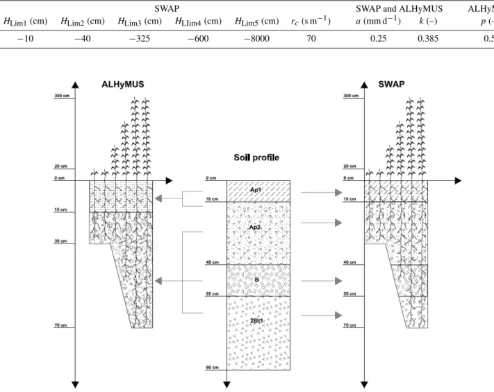
The soil profile schematization adopted by the two mod-els is illustrated in Fig. 2. For the SWAP model all the four soil horizons were taken into account, having the main prop-erties listed in Table 2. Soil hydraulic parameters for each horizon were determined using the five methods illustrated above. ALHyMUS considers two reservoirs in cascade in the root-zone: for each reservoir soil hydraulic parameters were computed from those determined for each horizon. In partic-ular, for all the parameters except for the saturated hydraulic conductivity, the arithmetic mean of the values of the soil hydraulic parameters of the horizons belonging to the reser-voir, weighted by their thickness, was calculated. For the vertical saturated hydraulic conductivity the harmonic mean was computed (e.g. Freeze and Cherry, 1979). For the case study, a simplified approach for the parameterization of the second reservoir was adopted, i.e. fixing the soil hydraulic parameters for the whole simulation period at the value ob-tained considering the maximum extension of the root zone (70 cm). Thus, the parameters for the second reservoir didn’t change over time with the roots’ growth.
Table 3.Crop parameters values used by SWAP and ALHyMUS models (variables are explained in the text).
SWAP SWAP and ALHyMUS ALHyMUS
HLim1(cm) HLim2(cm) HLim3(cm) HLIim4(cm) HLim5(cm) rc(s m−1) a(mm d−1) k(–) p(–)
−10 −40 −325 −600 −8000 70 0.25 0.385 0.5
Fig. 2.Experimental soil profile and its schematization in ALHyMUS and SWAP models (the horizons are coded using the USDA system).
probe (i.e. extending above and below the probe for half the distance to the next probe). A weighted average was then performed to calculate the initial water content for the two reservoirs.
The bottom boundary condition was prescribed for both models according to daily measurements of groundwater ta-ble depth from the ground surface, which showed variations in the range 80–120 cm during the simulation period. 2.6 Performance evaluation
SWAP and ALHyMUS were implemented with the five dif-ferent sets of soil hydraulic parameters described above re-sulting in a total of ten model-data sets, as summarized in Table 4. Daily measurements of evapotranspiration, average soil moisture in the root zone and flux at the root zone bottom collected in the field were used to test the performance of the
five methods and of the two models. The statistical evalua-tion was carried out using the normalized root mean square error (NRMSE) and the mean error (ME) calculated from simulated and observed daily values for the period 6 June to 10 October 2006 (DoY=157–283) respectively as:
NRMSE=RMSE
σ =
v u u u u u u t
N
P
i=1
(si−mi)2
N
P
i=1
(mi− ¯m)2
(4)
ME= 1 N
N
X
i=1
(si−mi) (5)
wheremi are the measured values,m¯ andσ their mean and
standard deviation,sithe simulated values, andNis the
Table 4.Summary of the simulations carried out for the performance analysis.
Code Description
M Measured values
S-Lab SWAP with parameters from laboratory measurements S-f SWAP with parameters from field measurements
S-H SWAP with parameters from the application of PTFs HYPRES S-RB SWAP with parameters from the application of PTFs of R&B S-Ro SWAP with parameters from the application of PTFs Rosetta A-Lab ALHyMUS with parameters from laboratory measurements A-f ALHyMUS with parameters from field measurements
A-H ALHyMUS with parameters from the application of PTFs HYPRES A-RB ALHyMUS with parameters from the application of PTFs of R&B A-Ro ALHyMUS with parameters from the application of PTFs Rosetta
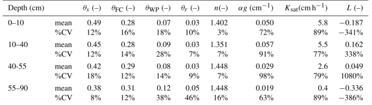
Table 5.Statistics for the soil hydraulic parameters determined using the five methods.
Depth (cm) θs(–) θFC(–) θWP(–) θr(–) n(–) αg(cm−1) Ksat(cm h−1) L(–)
0–10 mean 0.49 0.28 0.07 0.03 1.402 0.050 5.8 −0.187
%CV 12% 16% 18% 10% 3% 72% 89% −341%
10–40 mean 0.45 0.28 0.09 0.03 1.351 0.057 5.5 0.162
%CV 12% 14% 28% 7% 7% 91% 77% 338%
40-55 mean 0.42 0.29 0.08 0.03 1.448 0.029 2.6 0.049
%CV 18% 12% 14% 9% 7% 98% 79% 1080%
55–90 mean 0.38 0.31 0.12 0.05 1.448 0.019 0.4 −0.336
%CV 8% 12% 38% 46% 16% 63% 89% −386%
Simulation is perfect (i.e.mi=si) if NRMSE is zero;
pre-dictions are worse than using the mean of observed values if NRMSE is greater than one. Simulation shows a systematic overestimation if ME is positive and a systematic underesti-mation if ME is negative.
The same indices were also used to compare pairs of sim-ulations obtained running either the same model with two different parameter sets, or the two models with the same pa-rameter set; in these casesmi andm¯ were simulated values
as well.
3 Results and discussion
3.1 Comparison of soil hydraulic parameters
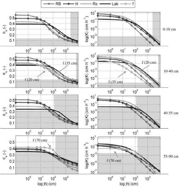
Table 5 shows means and variations coefficient for the pa-rameters determined using the five methods. Figure 3 illus-trates the retention and the hydraulic conductivity functions at different depths obtained by introducing soil hydraulic pa-rameters into the equations of van Genuchten (1980) and Mualem (1976) respectively.
There are different degrees of variation in the hydraulic parameters; such variation is exceptionally large for the satu-rated hydraulic conductivityKsat(cm h−1) and for the shape
parameterα(cm−1). The parameterL(–) also shows a high
variability but it is demonstrated that hydrological models are generally less sensitive to its variations (e.g. Jhorar et al., 2004).
Concerning the retention curves, PTFs RB in most of cases predict larger θs than the other methods. Due to relatively
highαandnvalues, causing a steep decline in the curve, the method nevertheless provides comparable or lower soil wa-ter contentsθfor high suction values. Similar observations apply toKsatand to the unsaturated conductivity curve. Also
in that case, due to the steepness of the curve,K(θ )values at higher suctions are comparable or even lower than those obtained by the other methods.
PTFs H result in lowerθs andKsatthan PTFs RB except
for the deeper horizon; but the overall patterns of retention and unsaturated conductivity curves are similar to those pre-dicted by the latter method. The curves generally show a more moderate and prolonged decline of water content and unsaturated conductivity with increasing suction.
The retention curves provided by PTFs Ro are generally characterized by lower values ofθsand a shape similar to the
curves predicted by PTFs H. The unsaturated conductivity curves are characterised by lower values ofKsatcompared to
55-90 cm 40-55 cm 10-40 cm 0-10 cm
f (20 cm)
f (35 cm)
f (70 cm) f (20 cm)
f (35 cm)
f (70 cm)
Fig. 3.Retention and hydraulic conductivity curves determined by using the five methods (for codes see Table 4) at the soil depths: 0–10 cm, 10–40 cm, 40–55 cm, 55–90 cm. Drier water contents/pressure heads – not observed in the field during the monitoring period – are shaded in gray.
The retention curves derived from laboratory measure-ments ofh−θ show smaller θs values than those given by
other methods, but generally they are characterized by a more moderate and prolonged decline of water content with in-creasing suction, leading to more elevated water contents at higher pressure heads than the other methods. The labora-tory θs values are even lower than the corresponding field
values, which is usually uncommon to find in the literature (e.g. Pachepsky et al., 2004; Leij et al., 1996). In this par-ticular case, it can be partially explained by the fact that the θs values of the field curves were actually determined in the
laboratory, on samples collected immediately after tillage ac-tivities were conducted (see Sect. 2.4.2). The unsaturated conductivity curves determined by the laboratory measure-ments are characterised by smaller values ofKsat in
com-parison with the other methods, except for the 4th layer for
which the value is considerably higher. However, in all the layers the values ofK(h)at high suction values are generally higher then those obtained with the other methods. As forθs
values,Ksatvalues were determined in laboratory on samples
collected before the soil tillage started.
The retention curves derived from field measurements of h−θ show values of θs within the range of those obtained
with the other methods, but the behaviour of the curves is quite peculiar. In the 2nd horizon, at the higherhvalues,θ (h) values tend to become higher than those derived by applying the other methods, while for the 4th horizon the opposite oc-curs. The unsaturated conductivity curves based on the field measurements are characterised by smaller values ofKsatin
comparison with those obtained by the other methods; only for the 2nd horizonKsat values are higher than laboratory
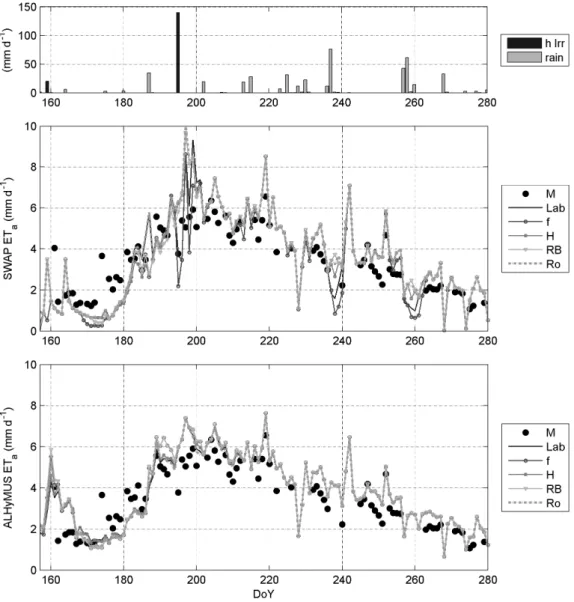
Fig. 4.Water inputs and evapotranspiration simulated by SWAP and ALHyMUS and measured by eddy-covariance (EC); for parameter sets codes see Table 4.
than those predicted with the other methods for the whole range ofh; for the 4th horizonK(h)increases at higher suc-tions in comparison for example to PTFs RB. It’s important to stress that since the soil water content in the field was al-ways relatively high during the monitoring period – and this was particularly true for deeper layers due to the presence of the shallow groundwater table – at higher suctions the repre-sentativeness of the two curves obtained from the field data can be questioned.
Although the collected data are not enough to state it doubtlessly, the direct comparison between field and labora-tory measurements suggested that a temporal variability in the soil hydraulic properties due to tillage practices could be present. Strudley et al. (2008) provided a detailed syn-opsis of the state-of-the-science for this issue and they ar-gued that more investigations should be conducted, since only “enhanced data collection and measurement campaigns,
combined with improved methods of parameter estima-tion and mechanistic incorporaestima-tion within explicit spatio-temporal modelling frameworks should aid in the under-standing of soil hydraulic behaviour due to tillage and related agricultural management.”
3.2 Performance evaluation
3.2.1 Evapotranspiration
of NRMSE are smaller then one. However, with all the soil hydraulic parameter sets and for both models, a systematic overestimation is shown (i.e. positive ME values in Fig. 9).
More insight can be achieved by splitting the cropping season into two periods. Simulation results for both SWAP and ALHyMUS show that the ratio of transpiration to evap-oration increases rapidly starting from about DoY 175 till DoY 186. It can be noted that this period falls a few days be-fore the main irrigation input occurs (between DoY 182 and DoY 195), when the soil is still relatively dry. Once these dates are reached, the agreement between measured and sim-ulated ET starts improving. The simulation period was there-fore split into a first part, where evaporation plays a major role, and a second one where transpiration is predominant.
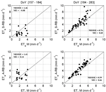
Figure 5 shows the measured evapotranspiration values vs. the simulated values obtained with the two models imple-mented with the RB parameter set when the two periods are considered. Similar results were obtained implementing the models with the other sets of soil hydraulic parameters. In the first period when the crop is small and soil evaporation is more important than crop transpiration (approximately from the emergence to the beginning of July), the fitting is poor (NRMSE=1.46 and 1.41 respectively for SWAP and ALHy-MUS). However, the systematic error in ALHyMUS is pos-itive but small (ME=0.14 mm d−1); on the contrary, SWAP underestimates the process (ME=−0.88 mm d−1).
In this first period the soil characteristics of the upper por-tion of the profile (i.e. 10–15 cm) and the water availabil-ity play the most important role in the determination of the evapotranspirative flux. The poor performance of the models is probably due to the presence of soil crusting and macro-porosity, which were noticed in the field but are not ac-counted for in the two models. However, further research is needed to better investigate this issue.
Regarding the differences between the results of the two models, it can be noted that ALHyMUS calculates the actual evaporation rate using the FAO Penman-Monteith equation with the dual crop coefficient approach of Allen et al. (1998) on the basis of the soil water content of the first soil layer, while SWAP adopts the original Penman-Monteith equa-tion and includes the procedure described in Kroes and van Dam (2003) to account for the limitations due to the water content in the upper portion of the soil profile. With these different setups generally ALHyMUS provides higher values of evapotranspiration rate than SWAP, as confirmed by an ex-tensive simulation exercise carried out with the two models considering different soil types and a 13-years simulation pe-riod (results not shown in this paper).
In the second period (from DoY-184 to 283), transpira-tion is the dominant process and the model performances improve (NRMSE=0.76 and 0.59 respectively for SWAP and ALHyMUS with the PTFs RB). However, both models show a systematic overestimation of the evapotranspirative flux (ME=0.68 mm d−1and 0.66 mm d−1respectively for SWAP and ALHyMUS). Different factors may have contributed to
NRMSE = 1.46 ME = - 0.88
NRMSE = 1.41 ME = 0.14
NRMSE = 0.76 ME = 0.68
NRMSE = 0.59 ME = 0.66
Fig. 5.Evapotranspiration measured by eddy-covariance (EC) and simulated by ALHyMUS and SWAP with the Rawls and Brakensiek parameter set (A-RB and S-RB respectively) for the period 3 June– 3 July and 3 July–10 October 2006.
these results, among which are the accuracy of crop pa-rameter values and the actual environmental conditions. In-deed, while nutrients limitation or soil salinization can be excluded, recent investigations in the area (e.g. Gerosa et al., 2003) showed that atmospheric pollution can inhibit the transpiration process; in particular, high ozone concentra-tions lead to a general reduction of the productivity (average crop yield loss of 5% for experiments conducted in open-top chambers) as well as to an increase of the crop sensitivity to other biotic and abiotic stresses.
A last consideration is that the SWAP results are highly variable after intense water inputs (e.g. days after the sur-face irrigation event: DoY=195 in Fig. 4) . This behaviour is due to the different effects of the restriction to the tran-spiration flux, performed by SWAP when the soil water con-tent is close to saturation, with the distinct parameter sets. Indeed, the limitation to transpiration is controlled by the pressure head thresholdsHLim1andHLim2, (see Table 3) and
the same parameter values have clearly a different impact on the results depending on the set of soil hydraulic parameters considered.
3.2.2 Soil water content
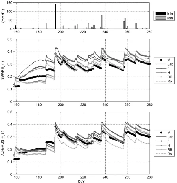
Fig. 6. Water inputs and average soil water content in the root zone simulated by SWAP and ALHyMUS and measured by soil moisture sensors; for parameter sets codes see Table 4.
content in the root zone was obtained by a weighted average of the measurements of the probes in the same day, where weights are proportional to the thickness of the layers. These average values, derived from measurements, will be simply indicated as measured values in the following.
The pattern of the simulated and measured values of the average soil moisture in the root zone and the corresponding efficiency indices are shown in Figs. 6 and 9, respectively. It can be noticed that both models show a high sensitivity to the different sets of hydraulic parameters. As documented in the literature (e.g. Coppola et al., 2009) both retention pa-rameters and hydraulic conductivity papa-rameters play a funda-mental role in determining the soil water content evolution, the former being dominant during drainage processes and the latter during infiltration processes. This case study is further complicated by the presence of a shallow groundwater table
which determines a water flux towards the root zone when the pressure head in proximity of the roots becomes particu-larly low.
very early stage of plant growth, and the rate of growth of the soil water content in the three simulations is larger than rate of growth of the measured values in the whole period between the simulation start and DoY 180. The opposite oc-curs with H and RB simulations, where the upward gradients are smaller, due to the different shapes of the initial head profiles deriving from the RB and H retention curves: the up-ward fluxes from underneath the root zone are very close to the evapotranspiration abstractions and hence the simulated soil moisture contents are relatively stable during the interval DoY 165–185 and lower than measured ones.
The performances achieved are in some cases very good for both SWAP and ALHyMUS: NRMSE of 0.53 and 0.43 and ME of −0.004 (m3m−3) and 0.011 (m3m−3) were found respectively with the parameter set of RB for the for-mer model and of Lab for the latter. Average water contents simulated by SWAP show a good agreement with the obser-vations also when the Ro parameter set is used, while ALHy-MUS provides good results also with both H and RB param-eter sets.
The range of variation of the two performance indices is quite large for both models (NRMSE 0.53 to 1.23 and ME−0.004 to 0.065 for SWAP; NRMSE 0.43 to 0.82 and ME−0.039 to 0.034 for ALHyMUS). Anyway, ALHyMUS proved to be less sensitive to the choice of the parameter set and provides values of NRMSE<1 in all cases.
It is worth observing that the performances of parame-ter sets derived by PTFs are similar to those of parameparame-ter sets obtained by direct methods. This is more evident in the case of the physically based SWAP model, for which val-ues of NRMSE higher than one were obtained by both di-rect methods (Fig. 9). It is commonly accepted that when the model parameters can be calibrated on the basis of local observations of soil moisture and pressure head, then phys-ically based models can provide better performances than conceptual models (e.g. van Dam et al., 2008; Coppola et al., 2009). Nevertheless, results of this study suggest that when the model parameters are derived from either direct or indirect methods, but no calibration is carried out, the perfor-mances of the two types of models can be quite similar. In the specific case study, ALHyMUS proved to be less sensi-tive to the parameter set and therefore to provide more ho-mogeneous results compared to SWAP. These considerations seem to indicate that, without calibration, there is no clear predominance of physically based over conceptual models and the use of PTFs based on site-specific physico-chemical data could be a practical choice.
NRMSE and ME indices were computed also by coupling in all possible ways the results of the different simulations carried out with the two models, using either the same model with two different parameter sets, or the two models with the same parameter set. In particular, differences in the results provided by the two models with the same data set could be read as a measure of the uncertainty in the results attributable to the modelling approach.
To this end, Fig. 7 shows the average soil water content in the root zone simulated by SWAP and ALHyMUS respec-tively with the RB parameter set (which provides the best fitting between the two models) and the Ro parameter set (worst fitting).
The first two graphs in the left column of Fig. 10 show the NRMSE and ME indices of the simulations A-RB and S-Lab, S-f, S-H, S-Ro, relative to the S-RB simulation. The RB parameter set provides the best agreement between SWAP and ALHyMUS results, which are closer (in terms of both NRMSE and ME) than the different SWAP simulations.
The third and fourth graphs in the left column of the same figure show the NRMSE and ME indices of the simulations A-Ro and S-Lab, S-f, S-H, S-RB, relative to the S-Ro sim-ulation. The Ro parameter set provides the worst agree-ment between SWAP and ALHyMUS results, and indeed both the NRMSE and ME values are worse for A-Ro than for the all the SWAP simulations, though the difference is not enormous.
Similar graphs, where the results of the S-Lab, S-f and S-H simulations are taken as reference patterns for NRMSE and ME computations, show an intermediate behaviour of these two indices, with an agreement of the SWAP and ALHyMUS simulations with the same parameter set often better than that of the SWAP simulations with the different parameter sets. Therefore, the analysis of the NRMSE and ME indices re-veals that the range of within model variability, due to the choice of a different parameter set for a given model, is of-ten wider than the range of inter-model variability, due to the choice of the model for a given parameter set.
3.2.3 Bottom flux
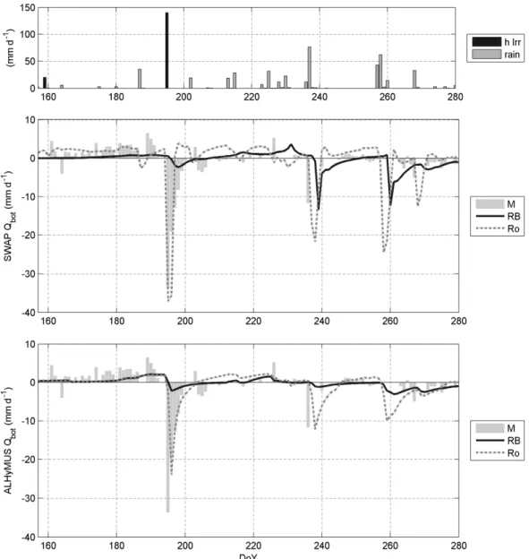
Figure 8 shows the comparison between the values simulated and “estimated from measurements” of the daily flux at the bottom of the root zone (whose depth increases from 30 to 70 cm during the crop growing stages, as shown in Fig. 1). The “estimated from measurements” values were obtained as residual terms of the daily hydrological balance computed by using the available measurements of soil water content and water inputs and outputs (i.e. rainfall, irrigation and evapo-transpiration).
Fig. 7. Water inputs and average soil water content in the root zone simulated by SWAP and ALHyMUS with the Rawls and Brakensiek (RB) and Rosetta (Ro) parameter sets.
to the one corresponding to PTFs RB, the pattern obtained by using the Lab parameter set is close to the one provided by PTFs Ro, while the one corresponding to the field parameter set shows rather an intermediate behaviour). Figure 9 reports the values of the efficiency indices calculated for all days in the simulation period in which the value of the “estimated from measurements” flux is available.
Although the number of “estimated from measurements” values is rather limited, Fig. 8 shows clearly that both mod-els succeed in capturing the general pattern of the bottom flux, but the overall performances are generally rather poor (i.e. NRMSE values between 0.6 and 1). As for the soil water content, it can be observed that SWAP shows a higher sensi-tivity to the choice of soil hydraulic parameters than ALHy-MUS does.
The best performances in terms of NRMSE are achieved in SWAP with the field parameter set and in ALHyMUS with the Ro parameter set, although the fluxes seem to be under-estimated also in these cases (negative ME values). Figure 8 shows that the highest percolation values during the infiltra-tion events are achieved, with both models, when the PTFs Ro are adopted. The reason of that was found, as in Soet and Stricker (2003), in the relatively flat shape of theK(θ ) curves near the saturation point, rather than to high values of Ksat. In all the other cases the simulated flux pattern turns
out to be more delayed and smoothened. This is particularly true when the PTFs RB are adopted. The unsaturated con-ductivity curves obtained with this parameter set are in fact characterized by generally high Ksat values, but also by a
Fig. 8.Water inputs and flow at the bottom of the root zone simulated by SWAP and ALHyMUS and estimated by hydrological balance (M); for graphical reasons only results obtained with RB and Ro parameter sets are shown.
When looking at the percolation outflow at the bottom of the profile simulated by ALHyMUS, the effects of smooth-ing and delaysmooth-ing of the inputs can be seen clearly (Fig. 8). This behaviour was already reported in literature for cascade reservoir models (e.g. Gandolfi et al., 2006) and it is a conse-quence of the simplified description of some of the processes, such as the percolation (i.e. unit gradient assumption). How-ever, looking at the patterns reported in Fig. 8 as well as at the NRMSE and ME indices, it cannot be concluded that AL-HyMUS generally performs worse than SWAP, the results depend greatly on the parameter set adopted.
As for soil water contents in the profile, NRMSE and ME were also computed for fluxes at the bottom of the profile by comparing the results obtained by the different parameter sets and simulation models in all possible ways. The right
Fig. 9. NRMSE and ME indices for evapotranspiration, average soil water content in the root zone and bottom flux outputs (simulated vs. measured values); for parameter sets codes see Table 4.
4 Summary and conclusions
This article investigates the uncertainty in modelling root zone water dynamics using two models of different complex-ity, SWAP, a Richards solver and ALHyMUS, a model based on a reservoir cascade scheme, in combination with Mualem-van Genuchten parameters determined by: i) parameter mization using laboratory measured data, ii) parameter opti-mization using field measured data, iii) PTFs of Rawls and Brakensiek (1989), iv) PTFs of HYPRES and v) PTFs of ROSETTA. Performance of the models was tested by the nor-malized root mean square error (NRMSE) and the mean error (ME) calculated from simulated and observed daily values of evapotranspiration, average root zone soil moisture content, and flux across the bottom of the root zone. The same in-dices were also computed by combining in all possible ways the results of the different simulations carried out with the two models, obtained running either the same model with two different parameter sets, or the two models with the same parameter set. Data used for this research were collected dur-ing an intensive monitordur-ing campaign at a 10 ha maize field located in Northern Italy, in the period June–October 2006.
The results show a high variability of the soil hydraulic parameter values in the different sets, especially in case of the saturated hydraulic conductivityKsat(cm h−1)and of the
shape parameter α(cm−1). Despite of this variability, the
Fig. 10. NRMSE and ME indices for the soil water content (1st column) and the bottom flux (2nd column) provided either using the two models (S orA) with the same parameter set or the same model with two different parameter sets. The reference patterns are those simulated by SWAP respectively adopting the PTFs RB (1st and 2nd rows) and Ro (3rd and 4th rows).
Both models show a high sensitivity to the choice of the set of soil hydraulic parameters when the average soil water content in the root zone and the flux at its bottom are consid-ered. However, ALHyMUS proved to be less sensitive to the choice of parameter set and therefore provides more homo-geneous results compared to SWAP.
When looking at the soil water content, both models repli-cate quite well the time pattern of observed soil moisture, though SWAP simulations show a systematic overestimation of soil moisture. The best performances are achieved for both SWAP and ALHyMUS with sets of hydraulic parameters ob-tained with indirect methods (PTFs), even if not necessarily the same set for the two models. Good results for ALHy-MUS are also achieved with the parameter set obtained from the laboratory data.
When the flux at the bottom of the root zone is considered, both models show a fairly good capability to capture the in-fluence of the shallow water table on the alternation of capil-lary rise and percolation fluxes at the bottom boundary over the simulation time, regardless of the parameter set. How-ever, the accuracy of the simulated values is generally rather poor. In many cases the patterns simulated by the two mod-els are delayed and smoothened in comparison with the data estimated from measured water balance components. This is particularly true in the case of ALHyMUS, as a consequence of the simplified representation of some of the processes in the soil profile, such as the percolation and the capillary rise. However, it cannot be concluded that ALHyMUS generally performs worse than SWAP, the results depend greatly on the parameter set adopted.
The simulation results show clearly that soil hydraulic pa-rameters obtained with direct methods do not necessarily guarantee the best performance. Indeed, for the specific case of the given experimental profile, the use of PTFs based on site-specific texture and organic matter data did provide com-parable results using both of the tested models. It can there-fore be stated that, at least for the case study, there is not a single method for the determination of soil hydraulic param-eters that is better than the others, and the suitability of a par-ticular method was also dependant on the type of simulation model that was used.
Moreover, the variability of the simulated average soil moisture and of the bottom flux due to the choice of the soil hydraulic parameter values is often larger than the dif-ference between the values of the same output variables sim-ulated by the two models adopting the same parameter set. This demonstrates that for these processes the choice of the method for deriving the values of the soil hydraulic parame-ters may be more important than the choice of the model.
It is commonly accepted that when the model parameters can be calibrated on the basis of local observations, then physically based models can provide a better performance than conceptual models do. Nevertheless, results of this study show that when the model parameters are derived from either direct or indirect methods, but no site-specific cali-bration is carried out, the performance of the two types of models can be very similar. In the authors opinion this is-sue deserves more research, since it could be very important, especially for large scale, spatially distributed model appli-cations.
by the results provided in this paper. We showed that a good agreement between the computed and observed values of the daily average soil water content in the root zone can be achieved, even if the evapotranspiration is overestimated and fluxes at the bottom of the root zone are underestimated. Clearly the errors in surface and bottom fluxes compensate each other, at least to a certain extent, and cannot be captured by looking just at soil moisture patterns. Therefore, multiple output variables should be considered for the evaluation of various parameterization methods and simulation models.
Acknowledgements. The research was financed by Fondazione
CARIPLO and MIUR-PRIN which are gratefully acknowledged. The authors wish to thank Nunzio Romano and his staff (DIAAT-University of Naples Federico II) for laboratory determinations of soil hydraulic properties and Roberto Comolli (DISAT-University of Milano-Bicocca) for support in soil characterization and sampling. Finally, the authors wish to thank the referees for their thoughtful and constructive comments.
Edited by: W. Durner
References
Allen, R., Pereira, L. S., Raes, D., and Smith, M.: FAO, Irrigation and drainage Paper 56, Crop evapotranspiration, Guidelines for computing crop water requirements, 1998.
Bastet, G., Bruand, A., Voltz, M., Bornand, M., and Qu´etin, P.: Performance of available pedotransfer functions for predicting the water retention properties of French soils, in: Characteri-zation and Measurement of the Hydraulic Properties of Unsat-urated Porous Media, edited by: van Genuchten, M. T., Leij, F. J., and Wu, L., University of California, Riverside, USA, 981– 991, 1999.
Belmans, C., Wesseling, J. C., and Feddes, R. A.: Simulation of the water balance of a cropped soil: SWATRE, J. Hydrol., 63, 271–286, 1983.
Borgarello, M., Catenacci, G., Cavicchioli, C., and Parini, S.: Indagini sulla deposizione secca, Rapporto CISE-SAA-93-042, CISE, Milano, 1993.
Bouma, J.: Using soil survey data for quantitative land evaluation. Adv. Soil Sci., 9, 177–213, 1989.
Bouma, J. and van Lanen, J. A. J.: Transfer functions and thresh-old values; from soil characteristics to land qualities, in: Quan-tified Land Evaluation, edited by: Beek, K. J., Burrough, P. A., and McCormack, D. E., International Institute Aerospace Sur-vey Earth Science, ITC Publishing, Enschede, The Netherlands, 106–110, 1987.
Bouraoui F. and Dillaha T. A.: ANSWERS-2000: Runoff and sedi-ment transport model, J. Environ. Eng., 6, 493–502, 1996. Braden, H.: Ein Energiehaushalts- und Verdunstungsmodell f¨ur
Wasser- und Stoffhaushaltsuntersuchungen landwirtschaftlich genutzer Einzugsgebiete, Mitteilungen der Deutschen Bo-denkundlichen Gesellschaft, 42, 294–299, 1985.
Christiaens, K. and Feyen, J.: Analysis of uncertainties associ-ated with different methods to determine soil hydraulic proper-ties and their propagation in the distributed hydrological MIKE SHE model, J. Hydrol., 246, 63–81, 2001.
Coppola, A., Basile, A., Comegna, A., and Lamaddalena, N.: Monte Carlo analysis of field water flow comparing uni and bi-modal effective hydraulic parameters for structured soil, J. Con-tam. Hydrol., 104(1–4), 153–165, 2009.
Cosby, B. J., Hornberger, G. M., Clapp, R. B., and Ginn, T. R.: A statistical exploration of the relationship of soil moisture charac-teristics to the physical properties of soils, Water Resour. Res., 20, 682–690, 1984.
Cresswell, H. P. and Paydar, Z.: Functional evaluation of methods for predicting the soil water characteristic, J. Hydrol., 227, 160– 172, 2000.
D’Urso, G. and Basile, A.: Physico-empirical approach for map-ping soil hydraulic behaviour, Hydrol. Earth Syst. Sci., 1, 915– 923, 1997,
http://www.hydrol-earth-syst-sci.net/1/915/1997/.
Eitzinger, J., Trnka, M., Hosch, J., Alud, Z., and Dubrovsky, M.: Comparison of CERES, WOFOST and SWAP models in simu-lating soil water content during growing season under different soil conditions, Ecol. Model., 171, 223–246, 2004.
ERSAL (Ente Regionale Sviluppo Agricolo Lombardo), Progetto carta pedologica – I suoli della pianura pavese centrale, Regione Lombardia, 2001.
Facchi, A., Ortuani, B., Maggi, D., and Gandolfi, C.: Coupled SVAT-groundwater model for water resources simulation in ir-rigated alluvial plains, Environ. Modell. Softw., 19(11), 1053– 1063, 2004.
Flanagan, D. C. and Livingston, S. J.: WEPP User Summary, NSERL Report No. 11., National Soil Erosion Research Labo-ratory, West Lafayette, 131 pp., 1995.
Freeze, R. A. and Cherry, J. A.: Groundwater, Prentice Hall Inc., Englewood Cliffs, New Jersey, 604 pp., 1979.
Gandolfi, C., Facchi, A., and Maggi, D.: Comparison of 1D models of water flow in unsaturated soils, Environ. Modell. Softw., 21, 1759–1764, 2006.
Gerosa, G., Cieslik, S., and Ballarin-Denti, A.: Micrometeorolog-ical determination of time integrated stomatal ozone fluxes over wheat: a case study in Northern Italy, Atm. Environm., 37(6), 777–788(C), 2003.
Gijsman, A. J., Jagtap, S. S., and Jones, J. W.: Wading through a swamp of complete confusion: how to choose a method for es-timating soil water retention parameters for crop models, Europ. J. Agronomy, 18, 77–106, 2003.
Goudriaan, J.: Crop meteorology: a simulation study, Simulation monographs, Pudoc, Wageningen, The Netherlands, 1977. Green, W. H. and Ampt, G.: Studies of soil physics. Part I. The flow
of air and water through soils, J. Agr. Sci, 4, 1–24, 1911. Guber, A. K., Pachepsky, Y. A., van Genuchten, M. Th., ˇSimnek, J.,
Jacques, D., Nemes, A. , Nicholson, T. J., and Cady, R. E.: Mul-timodel simulation of water flow in a field soil using pedotransfer functions, Vadose Zone J., 8(1), 1–10, 2009.
Guswa, A. J., Celia, M. A., and Rodriguez-Iturbe, I.: Models of soil moisture dynamics in ecohydrology: a comparative study, Water Resour. Res., 38(2), 1–15, 2002.
Haverkamp, R., Debionne, S., Viallet, P., Angulo-Jaramillo, R., and de Condappa, D.: Soil Properties and Moisture Movement in the Unsaturated zone, in: Handbook of Groundwater Engineering, The Second Edition, edited by: Delleur, J. W., Springer, Heidel-berg, 2006.
Herbst, M., Fialkiewicz, W., Chen, T., Putz, T., Thi´ery, D., Mouvet, C., Vachaud, G., and Vereecken, H.: Intercomparison of Flow and Transport Models Applied to Vertical Drainage in Cropped Lysimeters, Vadose Zone J., 4, 240–254, 2005.
Hupet, F., van Dam, J. C., and Vanclooster, M.: Impact of within-field variability in soil hydraulic properties on transpiration fluxes and crop yields: a numerical study, Vadose Zone J., 3, 1367–1379, 2004.
Huygen, J. C., van Dam, J. C., Kroes, J. G., and Wesseling, J. G.: SWAP 2.0: input and output manual, Technical document, WAU and DLO-Staring Centrum, Wageningen, 1997.
Islam, N., Wallender, W. W., Mitchell, J. P., Wicks, S., and Howitt, R. E.: Performance evaluation of methods for the estimation of soil hydraulic parameters and their suitability in a hydrologic model, Geoderma, 134, 135–151, 2006.
Jeffrey, D. W.: A note on the use of ignition loss as a means for the approximate estimation of soil bulk density, J. Ecology, 58, 297–299, 1970.
Johnson, H. and Jansson, P. E.: Water balance and soil moisture dynamics of field plots with barley and grass ley, J. Hydrol., 129, 149–173, 1991.
Johrar, R. K., van Dam, J. C., Bastiaansan, W. G. M., and Feddes, R. A.: Calibration of effective soil hydraulic parameters of het-erogeneous soil profiles, J. Hydrol., 285, 233–247, 2004. Kroes, J. G. and van Dam, J. C.: Reference Manual SWAP version
3.0.3, Alterra-rapport 773, ISSN 1566–7197, 2003.
Lamorski, K., Pachepsky, Y., Slawinski, C., and Walczak, R. T.: Us-ing Support Vector Machines to Develop Pedotransfer Functions for Water Retention of Soils in Poland, Soil Sci. Soc. Am. J., 72, 1243–1247, 2008.
Leij, F. J., Alves, W. J., van Genuchten, M. Th., and Williams, J. R.: The UNSODA-Unsaturated Soil Hydraulic Database. User’s manual Version 1.0. Report EPA/600/R-96/095, National Risk Management Research Laboratory, Office of Research and De-velopment, US Environmental Protection Agency, Cincinnati, OH, 1996.
Liu, Y., Pereira, L. S., and Fernando, R. M.: Fluxes through the bottom boundary of the root zone in silty soils: parametric ap-proaches to estimate groundwater contribution and percolation, Agric. Water Manag., 84, 27–40, 2006.
Maraux, F., Lafolie, F., and Bruckler, L.: Comparison between mechanistic and functional models for estimating soil water bal-ance: deterministic and stochastic approaches, Agric. Water Manag., 38, 1–20, 1998.
Minansy, B. and McBratney, A. B.: The Neur-N method for fitting neural network parametric pedotransfer functions, Soil Sci. Soc. Am. J., 66, 352–361, 2002.
Monteith, J. L.: Evaporation and the Environment, in: The state and movement of water in living organisms, edited by: Fogg, G. E., Cambridge University Press, 205–234, 1965.
Mualem, Y.: A new model for predicting the hydraulic conductivity of unsaturated porous media, Water Resour. Res., 12, 513–522, 1976.
Neitsch, S., Arnold, J., Kiniry, J., Srinivasan, R., and Williams, J.: Soil and water assessment tool users manual version 2000, GSWRL report 02-02, BRC report 02-06, Texas Water Re-sources Institute, College Station, TX, 2002.
Nemes, A., Schaap, M. G., and W¨osten, J. H. M.: Functional eval-uation of pedotransfer functions derived from different scales of data collection, Soil Sci. Soc. Am. J., 67, 1093–1102, 2003. Nemes, A., Wosten, J. H. M., Bouma, J., and Varallyay, G.: Soil
water balance scenario studies using predicted soil hydraulic pa-rameters, Hydr. Proc., 20, 1075–1094, 2006a.
Nemes, A., Rawls, W. J., and Pachepsky, Y. A.: Use of the Nonpara-metric Nearest Neighbor Approach to Estimate Soil Hydraulic Properties, Soil Sci. Soc. Am. J., 70, 327–336, 2006b.
Nemes, A., Rawls, W. J., Pachepsky, Y. A., and van Genuchten, M. Th.: Sensitivity Analysis of the Nonparametric Nearest Neighbor Technique to Estimate Soil Water Retention, Vadose Zone J., 5, 1222–1235, 2006c.
Niswonger, R., Prudic, D., and Regan, R.: Documentation of the unsaturated zone flow (UZF1) package for modeling unsaturated flow between the land surface and the water table with MOD-FLOW, Tech. Meth. 6-A19, USGS, 965 Reston, VA, 2006. Pachepsky, Y. A. and Rawls, W. J.: Accuracy and reliability of
pe-dotransfer function as affected by grouping soils, Soil Sci. Soc. Am. J., 63, 1748–1757, 1999.
Pachepsky, Y. A., Smettem, K. R. J., Vanderborght, J., Herbst, M., Vereecken, H., and W¨osten, J. H. M.: Reality and fiction of mod-els and data in soil hydrology, in: Unsaturated-Zone Modelling, edited by: Feddes, R. A., de Rooij, G. H., and van Dam, J. C., Kluwer Academic Publishers, Dordrecht, The Nederlands, 2004. Rawls, W. J. and Brakensiek, D. L.: Estimation of soil water reten-tion and hydraulic properties, in: Unsaturated flow in hydrologic modelling, Theory and Practice, edited by: Morel-Seytoux, H. J., Kluwer Academic Publishers, 275–300, 1989.
Refsgaard, J. C. and Storm, B.: MIKE SHE, in: Computer models of watershed hydrology, edited by: Singh, V. P., Water Resour, Publ., Littleton, CO, 809–846, 1995.
Reynolds, W. D., Elrick, D. E., Youngs, G., Booltink, H. W. G., and Bouma, J.: Saturated and field-saturated water flow parameters: laboratory methods, in: Methods of Soil Analysis, Part 4, 2002. Romano, N., Hopmans, J. W., and Dane, J. H.: Water retention
and storage: Suction table, in: Methods of Soil Analysis, Part 4, Physical Methods, edited by: Dane, J. H. and Topp, G. C., SSSA Book Series N.5, Madison, WI, USA, ISBN 0-89118-841-X, 692–698, 2002.
Richards, L. A.: Capillary conduction of liquids through porous mediums, Physics, 1, 318–333, 1931.
Romano, N.: Water retention and movement in the soil, in: CGIR Handbook of Agricultural Engineering, ASAE, 1999.
Saxton, K. E. and Rawls, W. J.: Soil water characteristic estimates by texture and organic matter for hydrologic solutions, Soil Sci. Soc. Am. J., 70, 1569–1578, 2006.
Schulla, J. and Jasper, K.: Model DescriptionWaSiM-ETH. Internal report, IAC, ETH Zurich, 166 pp., 2001.
Sharpley, A. N. and Williams, J. R.: EPIC Erosion Productivity Impact Calculator: 1. Model documentation, ARS-31, USDA, 1990.
Simunek, J., Huang, K., and van Genuchten, M. Th.: The HYDRUS Code, Research Report No. 144, US Salinity Laboratory Agricul-tural Research Service, USDA, Riverside, California, 1998. Soet, M. and Stricker, J. N. M.: Functional behaviour of
pedotrans-fer functions in soil water flow simulation, Hydrol. Process., 17, 1659–1670, 2003.
Starks, P. J., Heathman, G. C., Ahuja, L. R., and Ma, L.: Use of limited soil property data and modeling to estimate root zone soil water content, J. Hydrol., 272, 131–147, 2003.
Stoppelenburg, F. J., Kovar, K., Pastoors, M. J. H., and Tiktak, A.: Modeling the interactions between transient saturated and unsat-urated groundwater flow. Off -line coupling of LGM and SWAP, Rep. 500026001, RIVM, Bilthoven, The Netherlands, 2005. Strudley, M. W., Green, T. R., and Ascough, J. C.: Tillage effects on
soil hydraulic properties in space and time: state of the science, Soil Till. Res., 99, 4–48, 2008.
Sudicky, E. A., Park, Y. J., Unger, A. J. A., Jones, J. P., Brookfield, A. E., Colautti, D., Therrien, R., and Graft, T.: Simulating com-plex flow and contaminant transport dynamics in an integrated surface–subsurface modeling framework., in GSA Annu. Meet. and Exposition, Philadephia, Geol. Soc. of Am., Boulder, CO, 38(7), p. 258, 2006.
Tietje, O. and Hennings, V.: Accuracy of the saturated hydraulics conductivity prediction by pedo-transfer function compared to the variability within FAO textural classes, Geoderma, 69, 71– 84, 1996.
Tietje, O. and Tapkenhinrichs, M.: Evaluation of pedo-transfer functions, Soil Sci. Soc. Am. J., 57, 1088–1095, 1993.
Twarakavi, N. K. C., Simunek, J., and Schaap, M. G.: Development of Pedotransfer Functions for Estimation of Soil Hydraulic Pa-rameters using Support Vector Machines, Soil Sci. Soc. Am. J., 73, 1443–1452, 2009.
Ungaro, F. and Calzolari, C., Using existing soil databases for es-timating retention properties for soils of the Pianura Padano-Veneta region of North Italy, Geoderma, 99, 99–121, 2001. Ungaro, F., Calzolari, C., and Busoni, E.: Development of
pedo-transfer functions using a group method of data handling for the soil of the Pianura Padano–Veneta region of North Italy: water retention properties, Geoderma, 124, 293–317, 2005.
van Dam, J. C., Huygen, J., Wesseling, J. G., Feddes, R. A., Ka-bat, P., Van Walsum, P. E. V., Groenendijk, P., and Van Diepen, C. A.: Theory of SWAP version 2.0. Simulation of water flow, solute transport and plant growth in the Soil-Water-Atmosphere-Plant environment, Report 71, Department of Water Resources, WAU, Technical Document 45, DLO Winand Staring Centre-DLO, 167 pp., 1997.
van Dam, J. C., Groenendijk, P., Hendriks, R. F. A., and Kroes, J. G.: Advances of Modeling Water Flow in Variably Saturated Soils with SWAP, Vadoze Zone J., 7, 640–653, 2008.
van Genuchten, M. Th.: A closed form equation for predicting the hydraulic conductivity of unsaturated soils, Soil Sci. Soc. Am. J., 44, 892–898, 1980.
van Genuchten, M. Th., Leij, F. J., and Yates, S. R.: The RETC code for quantifying the hydraulic functions of unsaturated soils, USEPA Rep. IAG-DW12933934, R.S. Kerr Environ. Res. Lab., US Environmental Protection Agency, Ada, OK, USA, 1991. Vereecken, H., Diels, J., van Orshoven, J., Feyen, J., and Bouma,
J.: Functional evaluation of pedotransfer functions for the esti-mation of soil hydraulic properties, Soil. Sci. Soc. Am. J., 56, 1371–1378, 1992.
Vereecken, H., Maes, J., and Darius, P.: Estimating the soil mois-ture retention characteristic from texmois-ture, bulk density and carbon content, Soil Sci., 148, 389–403, 1989.
Workmann, S. R. and Skaggs, R. W.: Sensitivity of water manage-ment models to approaches for determining soil hydraulic prop-erties, Transaction of the ASAE, 37(1), 95–102, 1994.
W¨osten, J. H. M., Bannink, M. H., de Gruijter, J. J., and Bouma, J.: A procedure to identify different groups of hydraulic conduc-tivity and moisture retention curves for soil horizons, J. Hydrol., 86, 133–145, 1986.
W¨osten, J. H. M., Lilly, A., Nemes, A., and Le Bas, C.: Develop-ment and use of a database of hydraulic properties of european soils, Geoderma, 90, 169–185, 1999.