Data Quality in Hybrid Neuro-Fuzzy based Soft-Sensor Models: An Experimental Study

Abstract—Soft sensor models are used to infer the critical process variables that are otherwise difficult, if not impossible, to measure in broad range of engineering fields. Adaptive Neuro-Fuzzy Inference System (ANFIS) has been employed to develop successful ANFIS based sensor models. In addition to the structure of the model, the quality of the training as well as of the testing data also plays a crucial role in determining the performance of the soft sensor. This paper investigates the impact of data quality on the performance of an ANFIS based soft sensor model that is designed to estimate the average air temperature in distributed heating systems. The average air temperature is estimated based upon the available information, including solar radiation (Qsol), energy used by boiler (Qin) and external temperature (T0). For this problem, with the measurement errors caused by reading and equipment of all three variables, it is not unusual to have some uneven patterns in dataset which will decrease the model accuracy. The article investigates the impact of data quality on the performance of the soft sensor model. The results of two experiments are reported. The results show that the performance of ANFIS based sensor models is sensitive to the quality of data. The paper also discusses how to reduce the sensitivity by an improved mathematical algorithm.

Index Terms— ANFIS-GRID, Data quality, Inferential control scheme, Soft sensor, Error rate, Magnitude of error

I. INTRODUCTION

Soft sensing allows difficult to measure process variables to be inferred from other easily made measurements [1]. All soft sensors are based on an inferential model that represents the dynamics between the inputs, or easily measurable variables, and the output, or undetectable variables. Listed below are some commonly used approaches for the development of the inferential modeling module:

• Physical Model

Manuscript received May 22, 2009. The work presented in this paper is partially funded by National Sciences and Engineering Research Council of Canada (NSERC) with research project reference number as: 313375-07, and is carried out at Ryerson University, Toronto, Canada. The support of this organization is gratefully acknowledged.

S. Jassar is with the Department of Electrical and Computer Engineering, Ryerson University, 350 Victoria Street, M5B2K3, Toronto, Canada. (corresponding author’s phone: 416-979-5000 ext 4223; e-mail: sjassar@ ryerson.ca).

Z. Liao is the Associate Professor with the department of Architectural Sciences, Ryerson University, 350 Victoria Street, M5B2K3, Toronto, Canada. (e-mail: zliao@ryerson.ca).

L. Zhao is the Associate Professor with the Department of Electrical and Computer Engineering, Ryerson University, 350 Victoria Street, M5B2K3, Toronto, Canada. (e-mail: lzhao@ ee.ryerson.ca).

• Neural Network

• Fuzzy Logic

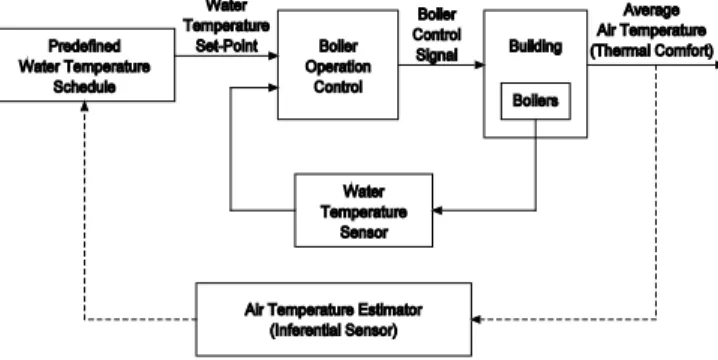
• Adaptive Neuro-Fuzzy Inference System (ANFIS) Recent research demonstrates the use of ANFIS in the development of a soft sensor model that estimated the average air temperature in a distributed heating system [2]. The estimated average air temperature allows for a closed-loop boiler control scheme (see the feedback loop through dashed line in Fig. 1), resulting in higher energy efficiency and improved comfort. In the current practice , due to the absence of economic and technically reliable method for measuring the overall comfort level in the buildings, the boilers are normally controlled to maintain the supply water temperature as a predefined level that normally does not reflect the heating demand of the buildings (see the solid feedback loop in Fig. 1) [3].

For ANFIS based soft sensor models, when estimation/prediction accuracy is concerned, it is assumed that both the data used to train the model and the testing data to make estimations are free of errors [4]. But rarely a dataset is clean before extraordinary effort having been made to clean the data. For this problem of average air temperature estimation, with the measurement errors in the input variables of the model, it is not unusual to have some uneven patterns in the dataset. This paper is aiming to analyze the impact of data quality of both training and testing datasets on the estimation accuracy of the developed model.

The paper is organized as follows. Section 2 will discuss the development of ANFIS based soft sensor model. Impact of data quality on ANFIS performance is analyzed in section 3. Results are presented in Section 4. Finally, conclusion of the research is given.

Fig. 1 Block diagram representation of closed-loop boiler control scheme.

Data Quality in Hybrid Neuro-Fuzzy based

Soft-Sensor Models: An Experimental Study

II. ANFIS BASED SOFT SENSOR MODEL

As an AI technique, “Soft Computing”, integrates powerful artificial intelligence methodologies such as neural networks and fuzzy inference systems. While fuzzy logic performs an inference mechanism under cognitive uncertainty, neural networks posses exciting capabilities such as learning, adaption, fault-tolerance, parallelism and generalization. Since Jang proposed ANFIS, its applications are numerous in various fields, including engineering, management, health, biology and even social sciences [5].

ANFIS is a multi-layer adaptive network-based fuzzy inference system. An ANFIS consists of a total of five layers to implement different node functions to learn and tune parameters in a fuzzy inference system (FIS) structure using a hybrid learning mode. In the forward pass of learning, with fixed premise parameters, the least squared error estimate approach is employed to update the consequent parameters and to pass the errors to the backward pass. In the backward pass of learning, the consequent parameters are fixed and the gradient descent method is applied to update the premise parameters. Premise and consequent parameters will be identified for membership function (MF) and FIS by repeating the forward and backward passes. ANFIS has been widely used in prediction problems and other areas.

ANFIS based soft sensor model developed in this research infers the average air temperature, Tavg, from three easily

measurable variables. The three variables are external temperature, T0, solar radiation, Qsol,and energy consumed by

the boilers, Qin [6]. The FIS structure is generated by Grid

partitioning method.

Grid partition divides the data space into rectangular sub-spaces using axis-paralleled partition based on pre-defined number of MFs and their types in each dimension. The wider application of grid partition in FIS generation is blocked by the curse of dimensions. The number of fuzzy rules increases exponentially when the number of input variables increases. For example, if there are m MFs for each input variable and a total of n input variables for the problem, the total number of fuzzy rules is mn. It is obvious that the wide application of grid partition is threatened by the large number of rules. According to Jang, grid partition is only suitable for cases with small number of input variables (e.g. less than 6). In this research, the average air temperature estimation problem has three input variables. It is reasonable to apply the grid partition to generate FIS structure, ANFIS-GRID. Fig. 2 shows the model structure for ANFIS-GRID.

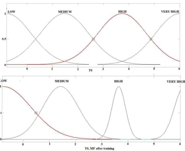
Gaussian type MFs, as shown in Fig. 3, is used for characterizing the premise variables. Each input has four MFs, thus there are 64 rules.

The developed structure is trained using hybrid learning algorithm. The parameters associated with the MFs change through training process. The shape of MFs also changes after training. This concept is clearly visible from the shape of MFs for T0 in Fig. 3. The shape of MFs for other two variables, Qin

and Qsol, is not clearly changed after training process, but the

associated parameters have changed significantly.

Fig. 3 MFs for Qin, Qsol and T0 before and after training

A.Training and Testing Data

Experimental data obtained from a laboratory heating system is used for training and testing of the developed model [7]. The laboratory heating system is located in Milan, Italy. The details of experimental data collection for the four variables, Qin, Qsol, T0 and Tavg, are given by the authors [2],

[6]. The dataset used for the training of ANFIS-GRID has 1800 input-output data pairs and is shown in Fig. 4.

The experimental data used for checking the performance of the developed model is shown in Fig. 5. The testing dataset has 7132 data pairs, which is large enough as compared to training dataset used for the development of the model.

0 500 1000 1500 2000 0

5000 10000 15000

Time (Hour of the Year)

Qi

n

(

W

)

0 500 1000 1500 2000 0

5000 10000 15000

Time (Hour of the Year)

Qso

l (

W

)

0 500 1000 1500 2000 -2

0 2 4 6

Time (Hour of the Year)

T

0 (

D

eg C

)

0 500 1000 1500 2000 16

18 20 22

Time (Hour of the Year)

T

avg

(

D

eg C

)

0 2000 4000 6000 8000 0

0.5 1 1.5

2x 10

4

Time( Hour of the Year)

Qi

n

(

W

)

0 2000 4000 6000 8000 0

5000 10000 15000

Time ( Hour of the Year)

Qso

l (

W

)

0 2000 4000 6000 8000 -5

0 5 10 15

Time (Hour of the Year)

T

0 (

D

eg C

)

0 2000 4000 6000 8000 16

18 20 22

Time (Hour of the Year)

T

avg

(

D

eg C

)

Fig. 5 Testing dataset (February 2000: day 1 to day 21)

III. IMPACT OF DATA QUALITY

Data quality is generally recognized as a multidimensional concept [8]. While no single definition of data quality has been accepted by the researchers working in this area, there is agreement that data accuracy, currency, completeness, and consistency are important areas of concern [9]-[12]. This study is primarily concerned about the data accuracy, defined as conformity between a recorded value and the corresponding actual data value.

Several studies have investigated the effect of data errors on the outputs of computer based models. Bansel et al. studied the effect of errors in test data on predictions made by neural network and linear regression models [13]. The training dataset applied in the research was free of errors. The research concluded that the error size had a statistically significant effect on predictive accuracy of both the linear regression and neural network models. O’Leary investigated the effect of data errors in the context of a rule-based artificial intelligence system [14]. He presented a general methodology for analyzing the impact of data accuracy on the performance of an artificial intelligence system designed to generate rules from data stored in a database. The methodology can be applied to artificial intelligence systems that analyze the data and generate a set of rules of the form “if X then Y”. It is often assumed that a subset of the generated rules is added to the system’s rule base on the basis of the measure of the “goodness” of each rule. O’Leary showed that the data errors can affect the subset of rules that are added to the rule base and that inappropriate rules may be retained while useful rules are discarded if data accuracy is ignored.

Wei et al. analyzed the effect of data quality on the predictive accuracy of ANFIS model [15]. The ANFIS model is developed for predicting the injection profiles in the Daqing Oilfields, China. As the study is using experimentally

collected data for training and testing of the ANFIS model, it is not unusual to have some extreme patterns in the dataset. The research analyzed the data quality using TANE algorithm. They concluded that the cleaning of data has improved the accuracy of ANFIS model from 78% to 86.1%.

In this research the experimental data collected from a laboratory heating system is used for training and testing of the developed ANFIS-GRID model. The data collected has some uneven patterns. In this section we will discuss the experiments conducted to examine the impact of data quality on the predictive performance of the developed ANFIS-GRID model.

A.Experimental Methodology

Data errors may affect the accuracy of the ANFIS based models in two ways. First, the data used to build and train the model may contain errors. Second, even if training data are free of errors, once the developed model is used for estimation tasks a user may use input data containing errors to the model. The research in this area has assumed that data used to train the models and data input to make estimation of the processes are free of errors. In this study we relax this assumption by asking two questions: (1) What is the effect of errors in the test data on the estimation accuracy of the ANFIS based models? (2) What is the effect of errors in the training data on the predictive accuracy of the ANFIS based models?

systematic data errors on the estimations made by the ANFIS based models.

Two experiments are conducted to examine the research targets. Both the experiments used the same application (estimation of average air temperature) and the same dataset.

Experiment 1 examines the first research question: What is the effect of errors in the test data on the estimation ability of the ANFIS based models? Experiment 2 examines the second research option: What is the effect of errors in the training data on the accuracy of the ANFIS based models?

B.Experimental Factors

There are two factors in each experiment: (1) fraction-error and (2) amount-error. Fraction-error is the percent of the data items in the appropriate part of the dataset (the test data in experiment 1 and the training data in experiment 2) that are perturbed. Amount-error is the percentage by which the data items identified in the fraction-error factor are perturbed.

Fraction-error

Since fraction-error is defined as a percent of the data items in a dataset, the number of data items that are changed for a given level of fraction-error is determined by multiplying the fraction-error by the total number of data items in the dataset.

Experiment 1

The test data used in experiment 1, shown in Fig. 5, has four data items (one value for each of the four input and output variables for one entry of the total 7132 data pairs). This experiment examines all of the possible number of data items that could be perturbed. These four levels for fraction-error factor are: 25% (one data item perturbed), 50% (two data items perturbed), 75% (three data items perturbed), and 100% (4 data items perturbed)

Experiment 2

The training data used in experiment 2 contains 1800 data pairs (one value for each of the four input and output variables for 1800 entries). Four levels of the fraction-error factor are tested: 5% (90 data items are perturbed), 10% (180 data items are perturbed), 15% (270 data items are perturbed), and 20% (360 data items are perturbed).

Amount-error

For both the experiments, the amount-error factor has two levels: (1) plus or minus 5% and (2) plus or minus 10%. The amount-error applied to the dataset can be represented by the following set of equations:

0.05

y

′ = ±

y

×

y

0.1

y

′ = ±

y

×

y

y

′

y

C.Experimental Design

The experimental design is shown in Table 1. Both the experiments have four levels for the fraction-error factor and two levels for the amount-error. For each combination of fraction-error and amount-error, four runs with random combinations of the input and output variable are performed.

Although the levels of the fraction-error are different in the two experiments, the sampling procedure is the same. For each fraction-error level, the variables are randomly selected to be perturbed. This is repeated a total of four times per level. Table 2 shows the combinations of the variables for experiment 1.

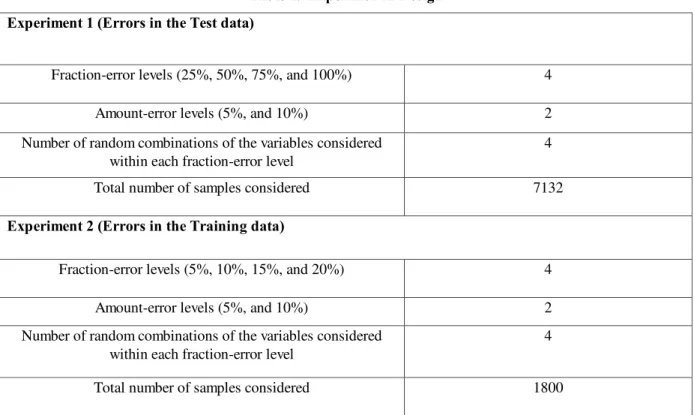
Table 1. Experimental Design Experiment 1 (Errors in the Test data)

Fraction-error levels (25%, 50%, 75%, and 100%) 4

Amount-error levels (5%, and 10%) 2

Number of random combinations of the variables considered within each fraction-error level

4

Total number of samples considered 7132

Experiment 2 (Errors in the Training data)

Fraction-error levels (5%, 10%, 15%, and 20%) 4

Amount-error levels (5%, and 10%) 2

Number of random combinations of the variables considered within each fraction-error level

4

Table 2. Four combinations of the variables for each fraction-error level in Experiment 1 Fraction-Error

Level

Input and Output Variable Combination

1 2 3 4

25%

( )

in

Q

( )

Q

( )

T

( )

50%

(

)

0

,

Q T

(

)

(

Q

,

T

)

(

)

75%

(

)

0

,

,

Q T Q

(

)

(

)

(

)

100%

(

)

in avg sol avg

Q T Q T

(

)

(

)

(

)

Table 3. Randomly assigned percentage increase (+) or decrease (-) for a given amount-error level in Experiment 1 Fraction-Error

Level

Input and Output Variable Combination

1 2 3 4

25%

( )

in

Q

-

(

Q

)

+

( )

T

+

( )

50%

(

)

0

,

Q T

+,-

(

)

(

Q

,

T

)

+,+

(

)

75%

(

)

0

,

,

Q T Q

+,-,-

(

)

(

)

(

)

100%

(

)

in avg sol avg

Q T Q T

-,+,-,+

(

)

(

)

(

)

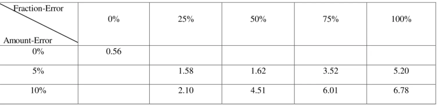
Table 4. Experiment 1 Results: RMSE (0C) Values as Error Level in the Test Data Varies Fraction-Error

Amount-Error

0% 25% 50% 75% 100%

0% 0.56

5% 1.58 1.62 3.52 5.20

10% 2.10 4.51 6.01 6.78

Table 5. Experiment 2 Results: RMSE (0C) Values as Error Level in the Training Data Varies Fraction-Error

Amount-Error

0% 5% 10% 15% 20%

0% 0.56

5% 2.32 1.62 1.58 7.20

Second, for each level of the amount-error factor, each variable is randomly assigned either a positive or negative sign to indicate the appropriate amount-error to be applied. Table 3 shows the randomly assigned amount-error levels in experiment 1. The procedure for experiment 2 differs only in the number of variables that were randomly selected to be perturbed for the four levels of the fraction-error factor.

D.Experimental Result

For both the experiments, the measured average air temperature values and ANFIS-GRID estimated average air temperature values are compared using Root Mean Square Error (RMSE) as a measure of estimation accuracy.

Experiment 1 Results: Errors in the Test Data

Estimation accuracy results, using the simulated inaccuracies for amount-error and fraction-error for the average air temperature estimation are given in Table 4. Table 4 shows that as fraction-error increases from 25% to 100%, RMSE increases indicating a decrease in predictive accuracy. As amount-error increases from 5% to 10%, RMSE increases also indicating a decrease in estimation accuracy. Both fraction-error and amount-error have an effect on predictive accuracy.

Experiment 1 Results: Errors in the Test Data

Predictive accuracy results, using the simulated inaccuracies for amount-error and fraction-error for the average air temperature estimation are given in Table 5. Table 5 shows that as fraction-error increases from 5% to 20%, RMSE increases indicating a decrease in predictive accuracy.

IV. TANE ALGORITHM FOR NOISY DATA DETECTION Data quality analysis results show that the errors in the training data as well as in the testing data affect the predictive accuracy of the ANFIS based soft sensor models. This section discusses an efficient algorithm, TANE algorithm, to identify the noisy data pairs in the dataset.

A.Functional Dependencies

The raw data is analyzed using approximate functional dependence mining method. An approximate dependency, or an approximate functional dependency, is a functional dependency that is almost valid with the exception of data tuples. A functional dependency studies the relationship of attributes in one or several tables, and claims that the value of an attribute is uniquely determined by the values of some other attributes. The discovery of functional dependencies in databases leads to useful knowledge and data quality problems.

More formally, a functional dependency over a relation is expressed as

X

→

A

⊆

R

A

⊆

R

r

t

u

∈

r

( )

[ ]

t B

=

u B

B

∈

X

t A

( )

=

u A

[ ]

X

→

A

A

∈

X

r

Approximate dependencies arise in many databases when there are natural dependencies between attributes, but some records contain errors and inconsistencies. For example, the relationship between zip code and the combination of city and state in a country. Another example is the social security number (SSN) and a corresponding person residing in the USA. Theoretically, these attributes have consistent relationships, as one person associated with one SSN, and one zip code associated with one combination of city, state in a country. But if errors are somehow introduced, the relationships between these attributes will be violated, which leads to the approximate dependencies.

B.TANE Algorithm

The TANE algorithm, which deals with discovering functional and approximate dependencies in large data files, is an effective algorithm in practice [16]. The TANE algorithm partitions attributes into equivalence partitions of the set of tuples. By checking if the tuples that agree on the right-hand side agree on the left-hand side, one can determine whether a dependency holds or not. By analyzing the identified approximate dependencies, one can identify potential erroneous data in the relations.

In this research, relationship of the three input parameters (Qin,

Qsol, and T0) and the average air temperature (Tavg) is analyzed

using TANE algorithm. For equivalence partition, all the four parameters are rounded off to zero decimal points.

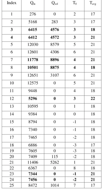
After data pre-processing, four approximate dependencies are discovered, as shown in Table 6. Although all these dependencies reflect the relationships among the parameters, the first dependency is the most important one because it shows that the selected input parameters have consistent association relationship with the average air temperature except a few data pairs, which is a very important dependency for average air temperature estimation.

To identify exceptional tuples by analyzing the approximate dependencies, it is required to investigate the equivalence partitions of both left-hand and right-hand sides of an approximate dependency. It is non-trivial work that could lead to the discovery of problematic data. By analyzing the first dependency, conflicting tuples are identified as some of them are given as bold entries in Table 7. From Table 7, one can see that detected tuples contain conflicting relationships or associations among parameter, and some of them contain severe ones. For example, as the same parameters in tuples 3 and 4, and tuples 7 and 8, the average air temperature values for these cases bear large difference. These data pairs could create trouble for average air temperature estimation. Based on the data trend, pairs 4, 7, 23, 24 are detected as conflicting tuples and are fixed using appropriate methodology. Table 2 shows only a small part of the total dataset. The total dataset has 7132 data pairs. For the first approximate dependency from Table 6, 42 conflicting data pairs are present which needs to be fixed for better performance of ANFIS-GRID model.

partitions attributes into equivalence partitions of the set of tuples. By checking if the tuples that agree on the right-hand side agree on the left-hand side, one can determine whether a dependency holds or not. By analyzing the identified approximate dependencies, one can identify potential erroneous data in the relations.

In this research, relationship of the three input parameters (Qin, Qsol, and T0) and the average air temperature (Tavg) is

analyzed using TANE algorithm. For equivalence partition, all the four parameters are rounded off to zero decimal points.

After data pre-processing, four approximate dependencies are discovered, as shown in Table 6. Although all these dependencies reflect the relationships among the parameters, the first dependency is the most important one because it shows that the selected input parameters have consistent association relationship with the average air temperature except a few data pairs, which is a very important dependency for average air temperature estimation.

Table 6. Approximate functional dependencies detected using the TANE algorithm

Index Approximate dependencies

Number of rows with conflicting tuples 1 Q Q_in, _sol,T₀→T_avg 42 2

0

,

,

in avg sol

Q T T

→

Q

3

0

,

,

in sol avg

Q Q

T

→

T

4

0

,

,

sol avg in

Q

T T

→

Q

V.RESULTS

A.Model Validation

The developed ANFIS-GRID model is validated using experimental results [7].The model performance is measured using the following statistical indices:

RMSE

(

)

RMS E T i T i

N =

=

∑

R2, Coefficient of determination, tells us how much of the experimental variability is accounted for by the estimate model.

2 2 1

2 1

ˆ ( )

( ) N avg avg i N avg avg i

T i T

R

T i T

= =  −    =  −   

∑

∑

, (4)

For equations (3) and (4),

N

T

ˆ

T

of average air temperature.

T

B.Results

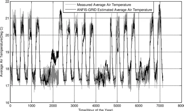
Initially, ANFIS-GRID model uses the raw data for both the training as well as the testing. Fig. 6 compares ANFIS-GRID estimated average air temperature values with the experimental results. ANFIS-GRID estimated average air temperature values are in agreement with the experimental results, with RMSE 0.560C. However there are some points at which estimation is not following the experimental results. For example, around 1900-2200 and 5100-5200 hour of the year time, there is a significant difference between estimated and experimental results.

For checking the effect of data quality on ANFIS-GRID performance, the training and testing datasets are cleaned using TANE algorithm. The conflicting data pairs are replaced with the required data pairs. Then the cleaned dataset is applied for the training and the testing of ANFIS-GRID model. A comparison of the model output with clean data and the experimental results is shown in Fig. 7.

Table7. Conflicting tuples identified by analyzing the first approximate dependency in Table 6

Index Qin Qsol T0 Tavg

1 276 0 2 17

2 5168 283 3 17

3 6415 4576 3 18

4 6412 4572 3 21

5 12030 8579 5 21

6 12601 4306 6 21

7 11778 8896 4 21

8 10501 8875 4 18

9 12651 3107 6 21

10 12575 0 5 21

11 9448 0 4 18

12 5296 0 3 22

13 10595 0 1 18

14 9384 0 0 18

15 8794 0 -1 18

16 7340 0 -1 18

17 7465 0 -2 18

18 6886 0 -3 17

19 7605 0 -3 18

20 7409 115 -2 18

21 11406 5262 1 21

22 6367 0 8 18

23 7344 0 -1 21

24 7456 0 -2 21

0 1000 2000 3000 4000 5000 6000 7000 8000 16

17 18 19 20 21 22

Time(Hour of the Year)

A

v

er

age A

ir

T

em

per

at

ur

e(

D

eg C

)

Measured Average Air Temperature

ANFIS-GRID Estimated Average Air Temperature

Fig. 6 Comparison of ANFIS-GRID estimated and measured average temperature values.

0 1000 2000 3000 4000 5000 6000 7000 8000

16 17 18 19 20 21 22

Time (Hour of the Year)

A

v

er

age A

ir

T

em

per

at

ur

e (

D

eg C

)

Measured Average Air Temperature

ANFIS-GRID Estimated Average Air Temperature

Fig. 8 Coefficient of determination with raw data

16.5 17 17.5 18 18.5 19 19.5 20 20.5 21 21.5

16.5 17 17.5 18 18.5 19 19.5 20 20.5 21 21.5

Measured Average Air Temperature ( Deg C )

E

s

ti

m

at

ed A

v

er

age A

ir

T

em

per

at

ur

e (

D

eg C

)

R-Square = 0.8945

Fig. 9 Coefficient of determination with clean data

16.5 17 17.5 18 18.5 19 19.5 20 20.5 21 21.5

16.5 17 17.5 18 18.5 19 19.5 20 20.5 21 21.5

Measured Average Air Temperature ( Deg C )

E

s

ti

m

at

ed A

v

er

age A

ir

T

em

per

at

ur

e (

D

eg C

)

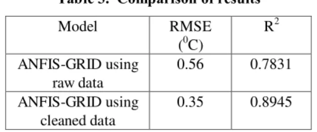
Table 3. Comparison of results

Model RMSE

(0C)

R2 ANFIS-GRID using

raw data

0.56 0.7831 ANFIS-GRID using

cleaned data

0.35 0.8945

Fig. 7 and Table 3 clearly show the effect of data quality on predictive accuracy of ANFIS-GRID model. The RMSE is improved by 37.5% to 0.350C. RMSE is considered as a measure of predictive accuracy. Less RMSE means less difference between the estimated values and the actual values. Finally, predictive accuracy is improved with decrease in RMSE. Fig. 8 and Fig. 9 show the improvement in R2 values.

VI. CONCLUSION

ANFIS-GRID based soft sensor model has been developed to estimate the average air temperature in distributed heating systems. This model is simpler than the subtractive clustering based ANFIS model [2] and can be used as the air temperature estimator for inferential control scheme for distributed heating systems (Fig. 1). Grid partition based FIS structure is used as there are only three input variables. The training dataset is also large enough as compared to the modifiable parameters of the ANFIS. As the experimental data is used for both the training as well as the testing of the developed model, it is expected that data can have some discrepancies. The discrepancies in the data can be the measurement errors due to reading and equipment. TANE algorithm is used to identify the approximate functional dependencies among the input and the output variables. The most important approximate dependency is analyzed to identify the data pairs with uneven patterns. The identified data pairs are fixed and again the developed model is trained and tested with the cleaned data. Table 3 shows that the RMSE is improved by 37.5% and R2 is improved by 12%. Therefore, it is highly recommended that the quality of datasets should be analyzed before they are applied in ANFIS based modelling.

Future work can be focused on analyzing the affect of adding feedback to ANFIS-GRID model. From the analysis, it can be concluded that if the model output is less sensitive to the errors in the dataset. Further research can be concentrated on the development of an adaptive and robust control scheme using the average air temperature estimator (Fig. 1).

ACKNOWLEDGEMENT

The work presented in this paper is partially funded by Natural Sciences and Engineering Research Council of Canada (NSERC) with research project reference numbers as: 313375-07 & 293237-09 and is carried out at Ryerson University, Toronto, Canada. The support of this organization is gratefully acknowledged.

REFERENCES

[1] M.T. Tham, G.A. Montague, A.J. Morris and P.A. Lant, “Estimation and inferential control”, Journal of Process Control, vol. 1, 1993, pp. 3-14. [2] S. Jassar, Z. Liao and L. Zhao, “Adaptive neuro-fuzzy based inferential sensor model for estimating the average air temperature in space heating systems”, Building and Environment, vol. 44, 2009, pp. 1609-1616. [3] Z. Liao and A.L. Dexter, “An experimental study on an inferential control

scheme for optimising the control of boilers in multi-zone heating systems”, Energy and Buildings, vol. 37, 2005, pp. 55-63.

[4] B.D. Klein, and D.F. Rossin, “Data errors in neural network and linear regression models: an experimental comparison”, Data Quality, vol. 5, 1999, pp 33-43.

[5] J.S.R. Jang, “ANFIS: Adaptive-network-based fuzzy inference system”,

IEEE Transactions on Systems, Man and Cybernetics, vol. 2, 1993, pp. 665-685.

[6] Z. Liao and A.L. Dexter, “A simplified physical model for estimating the average air temperature in multi-zone heating systems”, Building and Environment, vol. 39, 2004, pp.1013-1022

[7] BRE, ICITE, “Controller efficiency improvement for commercial and industrial gas and oil fired boilers”, A craft project, Contract JOE-CT98-7010, 1999-2001.

[8] J. Wang and B Malakooti, “A feed forward neural network for multiple criteria decision making”, Computers and Operations Research, vol. 19, 1992, pp. 151-167

[9] D. Ballou and H. Pazer, “Modeling data and process quality in Multi-Input, Multi-Output Information Systems”, Management Science,

vol. 31, 1985, pp. 150-162

[10] Y. Huh, F. Keller, T. Redman and A. Watkins, “Data Quality”,

Information and Software Technology, vol. 32, 1990, pp. 559-565 [11] E. Masson and Y Wang, “Introduction to Computation and Learning in

Artificial Neural Networks”, European Journal of Operational Research, vol. 47, 1982, pp. 37-42

[12] C. Fox, A. Levitin and T Redman, “The Notion of Data and Its Quality Dimensions”, Information Processing and management, vol. 30, 1993, pp. 9-19

[13] A. Bansal, R. Kauffman, and R. Weitz, “Comparing the mode ling performance of regression and neural networks as data quality varies”,

Journal of Management Information Systems, vol. 10, 1993, pp. 11-32. [14] D. O’Leary, “The impact of data accuracy on system learning”, Journal

of Management Information Systems, vol. 9, 1993, pp. 83-98. [15] M. Wei et al.’ Predicting injection profiles using ANFIS”, Information

Sciences, vol. 177, 2007, pp. 4445-4461.