Geosci. Model Dev., 6, 929–960, 2013 www.geosci-model-dev.net/6/929/2013/ doi:10.5194/gmd-6-929-2013
© Author(s) 2013. CC Attribution 3.0 License.
Geoscientiic
Model Development
Open Access
Geoscientiic
The SURFEXv7.2 land and ocean surface platform for coupled or
offline simulation of earth surface variables and fluxes
V. Masson1, P. Le Moigne1, E. Martin1, S. Faroux1, A. Alias1, R. Alkama1, S. Belamari1, A. Barbu1, A. Boone1, F. Bouyssel1, P. Brousseau1, E. Brun1, J.-C. Calvet1, D. Carrer1, B. Decharme1, C. Delire1, S. Donier1, K. Essaouini2, A.-L. Gibelin1,*, H. Giordani1, F. Habets3, M. Jidane2, G. Kerdraon1, E. Kourzeneva4,5, M. Lafaysse1, S. Lafont1, C. Lebeaupin Brossier1, A. Lemonsu1, J.-F. Mahfouf1, P. Marguinaud1, M. Mokhtari6, S. Morin1, G. Pigeon1, R. Salgado7, Y. Seity1, F. Taillefer1, G. Tanguy1, P. Tulet8, B. Vincendon1, V. Vionnet1, and A. Voldoire1 1CNRM/GAME, UMR3589, M´et´eo-France, CNRS, Toulouse and Grenoble, France
2CNRM, Direction de la M´et´eorologie nationale, Casablanca, Morocco
3UMR-SISYPHE, (UPMC, CNRS), Mines-Paristech, Centre de G´eosciences, Fontainebleau, France 4Russian State Hydrometeorological University, Malookhtisky Pr., 98, 195196, Saint Petersburg, Russia 5Finnish Meteorological Institute, P.O. Box 503, 00101, Helsinki, Finland
6Office National de la M´et´eorologie (ONM), Algiers, Algeria 7Centro de Geofisica de Evora, University of Evora, Evora, Portugal
8LACy, UMR8105, Universit´e de La R´eunion, CNRS, M´et´eo-France, Saint-Denis, France *now at: the Direction de la Climatologie, M´et´eo-France, Toulouse, France
Correspondence to:E. Martin ([email protected])
Received: 30 August 2012 – Published in Geosci. Model Dev. Discuss.: 21 November 2012 Revised: 30 April 2013 – Accepted: 27 May 2013 – Published: 16 July 2013
Abstract.SURFEX is a new externalized land and ocean sur-face platform that describes the sursur-face fluxes and the evo-lution of four types of surfaces: nature, town, inland water and ocean. It is mostly based on pre-existing, well-validated scientific models that are continuously improved. The moti-vation for the building of SURFEX is to use strictly identi-cal scientific models in a high range of applications in order to mutualise the research and development efforts. SURFEX can be run in offline mode (0-D or 2-D runs) or in coupled mode (from mesoscale models to numerical weather predic-tion and climate models). An assimilapredic-tion mode is included for numerical weather prediction and monitoring. In addition to momentum, heat and water fluxes, SURFEX is able to sim-ulate fluxes of carbon dioxide, chemical species, continental aerosols, sea salt and snow particles. The main principles of the organisation of the surface are described first. Then, a survey is made of the scientific module (including the cou-pling strategy). Finally, the main applications of the code are summarised. The validation work undertaken shows that re-placing the pre-existing surface models by SURFEX in these
applications is usually associated with improved skill, as the numerous scientific developments contained in this commu-nity code are used to good advantage.
1 Introduction
For these reasons, surface models continue to increase in complexity and accuracy as a result of improvements to ex-isting process parameterization or the addition of new pro-cesses. Examples of such models include CLASS (Verseghy et al., 1991), CLM (Lawrence et al., 2011), JULES (Best et al., 2011; Clark et al., 2011), LIS (Kumar et al., 2006), Noah (Ek et al., 2003), ORCHIDEE (Krinner et al., 2005), and TESSEL (Balsamo et al., 2009). Much effort has been put into the development of land data assimilation systems at various scales: from continental scale (e.g. Mitchell et al., 2004) to global scale (e.g. Rodell et al., 2004), based on var-ious land-surface models. The recent improvements in these models draw more and more benefits from multidisciplinary research and need highly flexible community codes so that the same code can be used for various applications. This is the only option if code duplications and errors in recoding between applications are to be avoided.
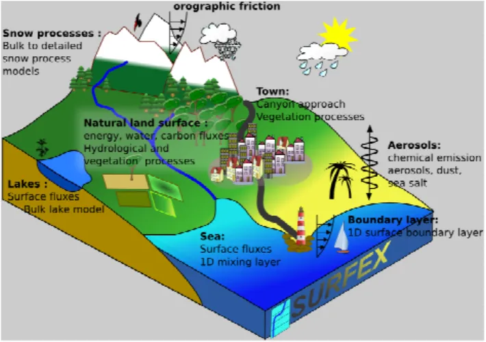
Taking advantage of the continuous development of the surface models ISBA (Noilhan and Planton, 1989) and TEB (Masson, 2000), and their coupling to both the atmospheric models Meso-NH (Lafore et al., 1998), ARPEGE (Courtier et al., 1991), ALADIN (Fischer et al., 2005), AROME (Se-ity et al., 2011; Brousseau et al., 2011), ALARO (Gerard et al., 2009; Hamdi et al., 2012), and the hydrological mod-els TRIP (Decharme et al., 2008) and MODCOU (Habets et al., 2008), the construction of a fully externalized surface scheme (i.e. a unique code that can be run in coupled and offline configurations) was undertaken. This surface scheme, SURFEX (from the French “Surface externalis´ee”; Fig. 1; www.cnrm.meteo.fr/surfex/), was built with the following specifications:
1. Include parameterizations for all components of the sur-face (ocean and land sursur-face, including urban areas and inland water) and simplified parameterizations for theo-retical studies.
2. Provide an interface with physiographic databases al-lowing the creation of various domain types (from point scale to various domain configurations).
3. Include a data assimilation component for numerical weather prediction applications and land-surface mon-itoring.
4. Preserve a single scientific code for all the surface ap-plications (offline or fully coupled with several atmo-spheric models).
An additional constraint in the building of SURFEX is that it is designed for a wide range of applications: point scale re-search simulation, 2-D offline applications at regional, con-tinental and global scale including the coupling with hydro-logical models, mesocale to global applications within vari-ous atmospheric models including operational weather pre-diction and long climate runs. Assimilation is used in both the numerical weather prediction chain and in the framework
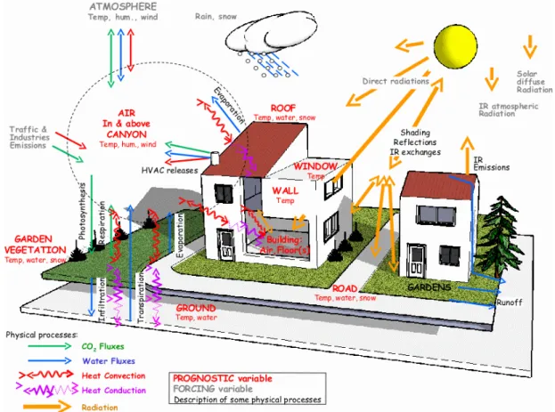
Fig. 1.Schematic representations of the main processes and func-tionalities of SURFEX.
of a land data assimilation system. The system needs to be modular, highly flexible with clearly specified interfaces.
The objective of this paper is to describe the present sta-tus of SURFEX (version 7.2). This is the first article of this type on SURFEX and it summarises the main features of the present state of the code, whose development began nearly 10 yr ago. The main principles of the model and the link with physiographic databases are described in Sects. 2 and 3, respectively. Then the physical schemes and their options are described in Sect. 4. Section 5 is devoted to chemistry, aerosols and sea salt. The strategy for coupling with atmo-spheric and hydrological models is described in Sect. 6. The assimilation is described in Sect. 7. Finally, Sect. 8 reviews the evaluation of the model and gives some examples of ap-plications.
2 Main principles of the model
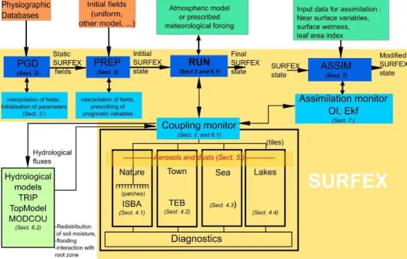
Due to its multiple uses, SURFEX is built in a modular way to allow an easy implementation of new technical and scien-tific features. The entry points of SURFEX are PGD (to pre-pare the physiographic data), PREP (to initialise prognostic variables), RUN (for offline and inline simulations) and AS-SIM (for assimilation Fig. 2.). The code is written in FOR-TRAN90, which is a higher level of the code using strict cod-ing norms identical for all tiles/patches and is devoted to the coupling with the atmosphere, aggregation/disaggregation of fluxes and the calling of the scientific models. Diagnostics are coded in a similar way for all tiles. Various input/ouput formats depending on the host model are available.
Fig. 2.Schematic representation of the main scientific and technical components of SURFEX (on a yellow background) and their interaction with other models and data.
are not yet parallelized, which is a limitation when SURFEX is used on large grids.
2.1 The tiling aproach
An accurate estimation of surface fluxes over a wide range of spatial resolutions needs to account for subgrid hetero-geneities (Essery et al., 2003). SURFEX offers the possibility to use tiles or to aggregate the surface parameters for lumped runs. Four main tiles are defined:
1. continental natural surfaces (“nature” tiles) including bare soils, rocks, permanent snow, glaciers, natural veg-etation and agricultural landscapes;
2. town (including buildings, roads and transportation in-frastructures, gardens);
3. inland water (including lakes and rivers); 4. sea and ocean.
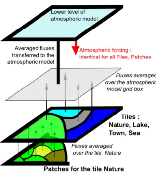
In order to account for heterogeneity within the continen-tal natural surfaces, this tile can be divided into “subtiles” (referred to as patches in what follows, Fig. 3.). A maximum of twelve patches which correspond to the plan functional types described in ECOCLIMAP (Table 1) can be described by SURFEX to account for the variety of soil and vegetation behaviour within a grid point. This allows non-vegetated sur-faces (bare soil, rocks, permanent snow) to be treated sepa-rately and accounts for the main plant functional types
(trop-Table 1.Patches used for the description of the nature continental tile.
Bare soil C3 crops Rocks C4 crops Permanent snow Irrigated crops Needle leaf trees Herbaceous Evergreen broadleaf trees Tropical herbaceous Deciduous broadleaf trees Wetlands
ical vs. temperate vegetation, low vs. tall vegetation, decid-uous vs. evergreen trees, various types of crops, etc.). In the tiling approach, each tile has the same meteorological forc-ing, while the model prognostic variables (liquid water con-tent, surface temperature, snow cover) and model parameters (soil depth, roughness length, LAI, etc.) and the correspond-ing fluxes are different.
Fig. 3.Schematic representation of the organisation of the surface using four main tiles and patches for nature (soil and vegetation tile).
3 Physiographic data
SURFEX is fully coupled with the global, 1 km resolu-tion, land cover database ECOCLIMAP. The original ver-sion (ECOCLIMAP1) is described by Masson et al. (2003). Versions with improvements over western Africa (Kaptu´e Tchuent´e et al., 2010) and Europe (Faroux et al., 2013) were developed later. The ECOCLIMAP database is composed of more than 550 cover types all over the world. Each cover is an ensemble of pixels with similar surface characteristics (e.g. sea, lakes, vegetated areas, suburban areas, etc.). They also account for the vegetation variability that depends on location, climate and phenology. This classification was es-tablished using land cover maps and satellite data.
The classification is complemented by look-up tables that allow the parameters for all physical schemes of SURFEX to be retrieved from the ECOCLIMAP covers:
1. Fraction of the surface occupied by each tile (sea, inland water, nature or town).
2. Urban parameters: characteristics concerning buildings and roads. vegetation properties of gardens.
3. Primary parameters for natural continental surfaces that depend on the cover and are defined for each of the 12 patches described in Table 1. These are the leaf area in-dex (LAI), the height of trees and the soil depth (surface, root and deep zones).
4. Secondary parameters that mainly depend on the patches (i.e. identical values for a given patch all over the world): vegetation fraction, emissivity, etc.
The covers are interpolated over the chosen grid. Then all urban, primary and secondary parameters are computed and aggregated if the number of patches is lower than 12. The town garden areas can be included in the nature tile or in the town tile (allowing for interaction with buildings). Some types of cover can be changed: lakes can be removed and replaced by nature and towns can be replaced by rocks.
Other physiographic datasets are needed by SURFEX: 1. Topography (e.g. Gtopo30 at 1 km, Gesch et al., 1999,
or SRTM, Farr et al., 2007, for higher resolution, from which the mean grid-cell altitude and sub-grid topogra-phy parameters are derived).
2. Soil properties (clay and sand proportions, organic mat-ter) derived from, e.g. FAO (FAO, 2006) or HWSD (Nachtergaele et al., 2012) databases.
3. Lake depth (Kourzeneva et al., 2012).
4. Ocean Bathymetry (e.g. Etopo2 by Smith and Sandwell, 1997).
The databases cited above are fully interfaced with SUR-FEX, but all parameters can be prescribed separately by the user. SURFEX is not limited to a particular database, hence databases other than those cited here can be used provided that they are put on a format that can be read by SURFEX.
4 Description of the physical models for land and ocean surface processes
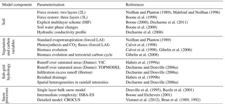
4.1 The Interaction Soil–Biosphere–Atmosphere (ISBA) land surface model
Table 2.Summary of the main parameterizations available in ISBA.
Model component Parameterisation References
Soil
Force restore: two layers (2L) Noilhan and Planton (1989), Mahfouf and Noilhan (1996) Force restore: three layers (3L) Boone et al. (1999)
Explicit multilayer scheme (DIF) Boone (2000), Decharme et al. (2011) Soil water phase changes Boone et al. (2000)
Hydraulic conductivity profile Decharme et al. (2006)
V
egetation
and
carbon
v
ariables
Standard evapotranspiration (forced LAI) Noilhan and Planton (1989) Photosynthesis and CO2fluxes (forced LAI) Calvet et al. (1998)
Biomass evolution Calvet et al. (1998), Gibelin et al. (2006) Biomass evolution and terrestrial carbon cycle Gibelin at al. (2008)
Sub-grid hydrology
Runoff over saturated areas (Dunne): VIC Habets et al. (1999a)
Runoff over saturated areas (Dunne): TOPMODEL Decharme and Douville (2006a) Infiltration excess runoff (Horton) Decharme and Douville (2006a) Residual drainage Habets et al. (1999b)
Spatial heterogeneities in rainfall intensities Decharme and Douville (2006a)
Sno
w
processes
Single layer bulk snow model Douville et al. (1995), Bazile et al. (2001) Intermediate complexity: ISBA-ES Boone and Etchevers (2001)
Detailed model: CROCUS Vionnet et al. (2012), Brun et al. (1989, 1992)
4.1.1 Surface energy budget
The ISBA surface energy budget is computed using a soil-vegetation composite approach. A single surface tempera-ture is used in the computation of the surface energy balance of the land/cover system (Noilhan and Planton, 1989). The surface heat flux,G(W m2), into this soil-vegetation-snow composite is equal to the sum of all the surface–atmosphere energy fluxes: the net radiation (Rn), the sensible heat flux (H) and the latent heat flux (LE). Rn is the sum of the net short-wave radiation and the net long-wave radiation com-puted using surface composite soil-vegetation-snow albedo and emissivity.His calculated by means of the Louis (1979) aerodynamics formulae depending upon the thermal stability of the atmosphere, modified by Mascart et al. (1995) in order to consider different roughness length for heat and momen-tum. Finally, LE is related to the sum of evaporation from the bare soil surface, sublimation from the snow pack and from soil ice, and evapotranspiration from the vegetation. More details can be found in Noilhan and Planton (1989), Douville et al. (1995) and Boone et al. (2000).
The surface soil-vegetation temperature (Ts) is approxi-mated as the temperature of a thin superficial layer having a depth fixed at 0.01 m. It varies according to the surface heat flux (G) and a soil heat flux. The latter depends on the soil scheme (see Sect. 4.1.2 for more details on the soil schemes). In the case of the force-restore approach (Noilhan and Plan-ton, 1989),Tsis restored towards its mean value over one day as proposed by Bhumralkar (1975) and Blackadar (1976). It also depends on the surface composite thermal inertia coef-ficient, which is parameterized as the harmonic mean of soil
(with or without soil ice), snow and vegetation thermal in-ertia coefficients (weighted by surface vegetation and snow fractions; Noilhan and Planton, 1989; Douville et al., 1995; Boone et al., 2000). If an explicit multi-layer soil scheme (Boone, 2000; Decharme et al., 2011) is used, the surface soil-vegetation temperature (Ts) varies according to the sur-face heat flux (G) and the soil heat flux calculated by com-bining the thermal gradient between the thin superficial layer and the second soil layer with the soil properties.
Surface energy budget in the presence of snow
In the case of one-layer bulk snow models, the force-restore composite surface temperature also accounts for snow. But when explicit multi-layer snow schemes are used (ISBA-ES or Crocus see Sect. 4.1.4), the surface energy budget is com-puted as the sum of the soil-vegetation composite energy budget and the snow energy budget weighted by the snow fraction (Boone and Etchevers, 2001). In this case, the “ra-diative” surface temperature is computed using the compos-ite soil-vegetation and the snow surface temperatures. This option is always used with the ISBA multi-layer soil diffu-sion scheme (Boone et al., 2000; Decharme et al., 2011). Note that bulk snow schemes cannot be used with explicit multi-layer soil schemes.
4.1.2 Soil
Force restore approach
so-called restore temperature is representative of the layer affected by a daily damping depth. For longer term simula-tions, there are two options to prevent model drift. The first method is to prescribe an external deep layer temperature. The restore temperature is itself restored to this temperature, which can be based on observational data and can be constant or time varying. The second method is a multilayer force-restore approach, each layer accounting for a given timescale (from 1 day to 1 yr). The latter method is applied for long cli-mate runs. Note that, in the configurations mentioned above, the thermal properties between the surface and the base of the restore layer(s) are assumed to be vertically homogeneous.
The vertical soil water transfer is represented by either two (2L) or three (3L) layers based on the force-restore method proposed by Deardorff (1977). The volumetric water content of the surface superficial layer (first layer) is restored towards the volumetric water content of the combined bulk surface and rooting layer (second layer). A set of force-restore co-efficients were computed by Noilhan and Planton (1989) us-ing hydraulic parameter values from Clapp and Hornberger (1978) based on either a simple analytical solution relying on Darcy’s law or a calibration using a high resolution one-dimensional model representation of Richard’s equation.
In addition to the classic force-restore approach described above, several improvements have been made. A gravita-tional drainage coefficient has been added, which relaxes the water content to the field capacity value when this value is ex-ceeded (Mahfouf and Noilhan, 1996), where the field capac-ity is the volumetric water content corresponding to a gravita-tional drainage of 0.1 mm day−1(Wetzel and Chang, 1987). The 3L version accounts for a third sub-root-zone layer to better represent the vertical soil moisture gradient in the va-dose zone, so an additional calibrated coefficient has been added to represent the diffusion between the root zone and the sub-root zones (Boone et al., 1999). If the water content of the bulk root or deep layers exceeds the soil porosity, a saturation excess runoff is generated. Note that this form of runoff is less likely when a sub-grid hydrological option is used (see Sect. 4.1.5). Finally, soil water can be extracted from the root zone for transpiration until the soil water de-creases to the wilting point volumetric water content (corre-sponding to a matrix potential of−15 bar). Bare soil evapo-ration can continue at water contents below wilting point, de-pending on both moisture and temperature, by water vapour transfer (Braud et al., 1993; Giard and Bazile, 1996). Finally, all force-restore coefficients and soil hydrological parameters are related to soil textural properties and moisture using the continuous relationships from Noilhan and Lacarr`ere (1995), which were derived from the Brooks and Corey (1966) model and the Clapp and Hornberger (1978) parameters (Noilhan and Planton, 1989; Noilhan and Mahfouf, 1996; Boone et al., 1999).
Explicit multilayer soil scheme
In contrast to the force-restore method, the surface and sub-surface layers are coupled via an explicit heat flux computa-tion based on the classical one-dimensional Fourrier law. The total soil heat capacity is computed as the sum of both wa-ter and soil matrix heat capacity. Following Johansen (1975), Farouki (1986) and Peters-Lidard et al. (1998), and the soil thermal conductivity is expressed as a function of volumetric water and ice contents, soil porosity and dry soil conductiv-ity. The surface and soil temperatures are computed using a method that permits fully implicit coupling with the atmo-sphere (see Sect. 6.1.1).
The explicit soil hydrology uses the so-called “mixed” form of the Richards equation to simulate the vertical water mass transfer within the soil via Darcy’s law. The water evo-lution is solved in terms of volumetric water, the hydraulic gradient being solved in terms of water pressure head. This mixed form is generally considered superior to the pressure-based or moisture-pressure-based forms because it maintains a high accuracy mass balance. In addition, the mixed form is ap-plicable to homogeneous or heterogeneous soils and to sat-urated or unsatsat-urated soils (Milly, 1985; Decharme et al., 2011). The relationship between soil moisture, soil matrix potential, and hydraulic conductivity is determined using the Brooks and Corey (1966) relationships. For dry soils, water vapour transfer can be significant and maintain evaporation from the soil. Therefore, vapour and liquid water conductiv-ity are summed, resulting in an effective conductivconductiv-ity. This depends on the soil texture, water content, and temperature (Braud et al., 1993). The water transfer between two layers depends on the inter-layer effective hydraulic conductivity (geometric mean between the conductivity of the two lay-ers). This method reduces the weighting error, improves the hydraulic transfer between layers, and is generally applica-ble in all situations of moisture gradient (Decharme et al., 2011). Water sinks include water extraction owing to evap-otranspiration and gravitational drainage. Soil evaporation is drawn from the superficial layer, while transpiration is re-moved throughout the root zone using an exponential distri-bution of roots (Jackson et al., 1996). Water sources include condensation on the surface layer, a possible mass influx at the lower boundary (when coupled to an aquifer model), and infiltration, which is parameterized via a Green and Ampt (1911) approach.
Most LSMs use a zero heat flux lower boundary condi-tion, the soil must be sufficiently deep with respect to the du-ration of the simulation in order to prevent model drift. For this reason, the soil thermal computations use additional lay-ers compared to the soil hydrological computational grid. To compute the heat capacity and thermal conductivity of these additional layers, the soil moisture is extrapolated downward assuming hydrostatic equilibrium in order to save computer time and while maintaining good hydrological simulations (e.g. river flow).
The default diffusion configuration of the model uses 14 layers to represent 12 m depth. Eight of these layers are in the top metre of the soil since Decharme et al. (2011) has shown that this was the minimum number of layers required to maintain a robust numerical solution of the Richards equa-tion.
Hydraulic conductivity profile
ISBA can account for the effect of soil heterogeneities on the vertical soil water transfer by using an exponential profile of the saturated hydraulic conductivity,ksat, with soil depth for both the force-restore and diffusion schemes. The main hy-pothesis is that roots and organic matter favour the develop-ment of macropores and enhance the water movedevelop-ment near the soil surface, and that soil compaction is an obstacle for vertical water transfer in the deeper soil. This parameteriza-tion (described in detail by Decharme et al., 2006) depends on only two parameters, which represent the rate of decline of theksat profile and the depth where ksat reaches its so-called “compacted value”. The first parameter can be related to soil properties but cannot exceed 2 m−1, and the second is assumed to be equal to the rooting depth. These two pa-rameters can also be tuned to improve streamflow forecasts (Quintana Segu´ı et al., 2009).
Soil water phase changes
Soil ice increases when water and energy are available for ice production. In contrast, the soil ice decreases due to melting and/or sublimation. During phase changes, the total soil wa-ter content for each soil layer is conserved, so as a soil freezes (resp. thaws), the liquid water content will decrease (resp. in-crease), corresponding to an increase (resp. decrease) in soil ice content. Since the surface is a composite layer, a surface insulation coefficient is introduced in order to partition the available energy into a portion which causes soil water phase changes and a part which heats or cools the vegetation (Gi-ard and Bazile, 2000). A characteristic timescale for phase changes is also introduced in order to prevent a time step dependence of the phase change. In order to avoid a compu-tationally intensive iterative solution procedure, the soil tem-perature profile is first calculated, then the phase change term is evaluated and temperatures are adjusted accordingly.
There are two methods available for soil water phase change. The first option corresponds to a simple energy-limited method (Giard and Bazile, 2000; Boone et al., 2000) which consists of freezing water whenever the soil tempera-ture falls below the freezing point, and melting soil ice when this temperature is exceeded. This simple method was de-veloped in order to reproduce the first-order effects of phase change on surface fluxes and lower atmospheric variables within the context of a force-restore approach. The second method determines a maximum liquid water content as a function of temperature using the Gibbs free energy con-cept (similar to that proposed by Cherkauer and Lettenmaier, 1999). Using this method, the soil phase changes follow the so-called soil specific freezing characteristic curve, so that liquid water can exist at sub-freezing temperatures. The re-lation between the soil water potential and temperature for sub-freezing conditions is from Fuchs et al. (1978), and the Brooks and Corey (1966) model is used to transform the soil matrix potential in the presence of ice into the maximum un-frozen (liquid) water content. This method is more physically based than the simple energy-limited method, and is more consistent with the multilayer soil option. It is better suited for longer timescale applications.
In terms of hydrology, soil ice has the effect of decreasing the hydraulic conductivity relative to a thawed soil with the same total soil moisture, since freezing–thawing can be mod-elled as drying–moistening to a good approximation (Kane and Stein, 1983; Spans and Baker, 1996). Therefore, as a soil freezes, ice is assumed to become part of the soil matrix, thereby reducing the soil porosity (Boone et al., 2000). Note that very large liquid water gradients can develop when sig-nificant soil water freezing occurs, so an ice impedance co-efficient is calculated following Johnsson and Lundin (1991) and used to prevent an overestimation of the upward liquid water flux at the freezing front.
4.1.3 Vegetation and carbon variables
Photosynthesis and CO2fluxes
models (Farquhar et al., 1980, for C3 plants and Collatz et al., 1992, for C4 plants) and it has the same formulation for C4 plants as for C3 plants, differing only by the input param-eters. Moreover, the slope of the response curve of the light-saturated net rate of CO2 assimilation to the internal CO2 concentration is represented by the mesophyll conductance (gm). Therefore, the value of the gm parameter is related to the activity of the Rubisco enzyme (Jacobs et al., 1996) while, in the model by Farquhar et al. (1980), this quantity is represented by a maximum carboxylation rate parameter VC,max. The model also includes a detailed representation of the soil moisture stress. Two different types of drought responses are distinguished for herbaceous vegetation (Cal-vet, 2000) and forests (Calvet et al., 2004), depending on the evolution of the water use efficiency (WUE) under moder-ate stress: WUE increases in the early soil wmoder-ater stress stages in the case of the drought-avoiding response, whereas it de-creases or remains stable in the case of the drought-tolerant response. In all cases, the soil moisture deficit impactsgm, which permits the limitation of photosynthesis during water stress to be described (Galle et al., 2009) in conjunction with other environmental factors such as leaf temperature or the leaf-to-air saturation deficit. It should be noted that, unlike the Jarvis-type parameterization used in the initial version of ISBA (Noilhan and Planton, 1989), the model parameters of heterogeneous grid-cells cannot be aggregated. Instead, sim-ulations must be performed over all patches.
Biomass evolution, carbon allocation and leaf phenology
ISBA-A-gs simulates the leaf biomass and the LAI (defined as the leaf area per unit ground area), using a simple growth model (Calvet et al., 1998). On a daily timestep, the leaf biomass is supplied with the carbon assimilated by photosyn-thesis during the course of the day, and decreased by turnover and respiration terms. LAI is inferred from the leaf biomass multiplied by the specific leaf area (SLA), which depends on the leaf nitrogen concentration (Calvet and Soussana, 2001; Gibelin et al., 2006).
Unlike most other land surface and vegetation models, there is no phenology module based on the accumulation of favourable days (like growing degree days for temperate deciduous phenology for instance). The phenology is directly the result of the photosynthetic activity and leaf mortality. Ecosystem respiration
The net ecosystem exchange (NEE) of CO2results from the balance between photosynthesis (or gross primary produc-tion, GPP) and the ecosystem respiration (Reco). In ISBA-A-gs, the latter is calculated using a simpleQ10response to soil temperature, weighted by surface soil moisture (Albergel et al., 2010a). For natural vegetation, the basal Reco rate can be calibrated to obtain an equilibrium between the accumu-latedRecoand GPP, on an annual or multi-annual basis. As
opposed to the ISBA-CC model (see below), the various au-totrophic and heterotrophic respiration terms are not calcu-lated.
Terrestrial carbon storage
Gibelin et al. (2008) developed the ISBA-Carbon Cycle (ISBA-CC) LSM in order to simulate the main components of the terrestrial carbon cycle. ISBA-CC is based on ISBA-A-gs and provides a number of additional variables represent-ing the vegetation biomass (wood and root compartments), the above- and below-ground litter pools and the soil car-bon pools. ISBA-CC uses the carcar-bon fluxes, and the leaf growth and senescence calculated by ISBA-A-gs to simulate the biomass in the wood and roots compartments. Biomass resulting from photosynthesis (minus leaf respiration) is first entirely allocated to leaves and twigs by the ISBA-A-gs mod-ule. It is then translocated to the other biomass pools at rates depending on the growth or senescence states of the plant, and the respiration of the pool. The litter and soil biogeo-chemistry module included in ISBA-CC is based on the well-known CENTURY model (Parton et al., 1987) that partitions the soil carbon among pools with different residence times. Since the autotrophic and heterotrophic respiration terms are calculated, the net primary production (NPP) can be sim-ulated. In the case of forests, the wood biomass growth is simulated and equilibrium climax biomass values can be de-termined. There is no representation of disturbance, whether natural or of human origin; for example, a forest manage-ment module would need to be implemanage-mented in order to rep-resent the carbon sink due to forest re-growth (Bellassen et al., 2010).
4.1.4 Snow
models for meso- to large-scale meteorological and hydro-logical applications, limiting the computation costs and sim-plifying the initialization issues (see Essery et al., 2013 for a comprehensive overview of the current state of the art of snow modelling). SURFEX currently contains three snow model options, which cover the entire spectrum of the model complexity mentioned above, and the users make their choice according to the scientific goals, computing resources and evaluation data available for a particular study.
Single layer bulk snow models
Two options using the so-called first-order schemes are avail-able (Douville et al., 1995; Bazile et al., 2001) and have been used extensively for global climate and numerical weather prediction applications. Both schemes use the composite-surface method based on the force-restore approach, and they contain three prognostic variables for a single-layer snow pack: the snow water equivalent (SWE), the average snow cover bulk density and an age-dependent snow albedo. Some noteworthy distinctions can be made between the two mod-els. In Douville et al. (1995), the surface thermal inertia in-cludes a contribution from the snow thermal properties, the minimum snow albedo is 0.50, the surface temperature used to compute snowmelt is linearly related to the restore tem-perature by the vegetation fraction, and the vegetation snow cover fraction depends on the vegetation aerodynamic rough-ness length. In Bazile et al. (2001), the surface thermal inertia is unchanged by the presence of a snow cover, the minimum snow albedo is 0.65, the snow-melt energy is directly com-puted using the surface temperature and the vegetation snow cover fraction depends on LAI and snow age. In both cases, in the presence of permanent snow or glacier, the minimum snow albedo is higher than in the case of seasonal snow. Intermediate complexity model: ISBA-Explicit snow
ISBA-Explicit Snow (ISBA-ES: Boone and Etchevers, 2001) was designed for implicit coupling with atmospheric mod-els and spatially distributed hydrological modelling applica-tions. There are three variables saved at each time step that are used to describe the state of the snow for multiple lay-ers: the heat content (or specific enthalpy), the snow den-sity, and the layer thickness. The snow albedo constitutes a fourth prognostic variable (which is the same as in Douville et al., 1995). In terms of the number of snow layers, the de-fault value is three (the minimum number to capture vertical gradients of density and temperature for most climate con-ditions) but some applications use up to 10 layers. Key pro-cesses represented include transmission of radiation within the snowpack, freeze-thaw, compaction and settling, and liq-uid water storage and through-flow. The snowpack is coupled to the underlying ground through a heat flux term in which the interfacial thermal conductivity represents both snow and soil-vegetation thermal properties.
Explicit internal-snow-processes model: Crocus
Crocus was primarily developed for the detailed study of the snowpack evolution at a particular location, and for op-erational avalanche prediction (Brun et al., 1989, 1992). It models the snow stratigraphy using a one-dimensional finite-element grid. The number of layers depends on a set of spe-cific rules intended to properly capture the snowpack layer-ing dynamics by representlayer-ing the vertical gradients of the snowpack with high resolution. Each snow layer is described by its thickness, temperature, density, liquid water content, grain types (dendricity, sphericity, size, and age), and a his-torical variable that indicates whether there has been liquid water or faceted crystals in the layer. In addition, Crocus takes the slope angle of the surface into account when puting the compaction. The impact of drifting snow on com-paction, metamorphism and sublimation can also be taken into consideration. Crocus has recently been rewritten to match the ISBA-ES structure and interfaces within SUR-FEX. The model is driven by meteorological variables ob-served, analysed, or modelled at the snow surface, or it can be implicitly coupled with an atmospheric model. The cou-pling with the underlying ground is identical to that used by ISBA-ES. See Vionnet et al. (2012) for an up to date, com-prehensive overview of Crocus in SURFEX.
4.1.5 Subgrid hydrology
At regional or global scale, the land surface water budget is calculated on grid cells with sides that typically measure from several km to 300 km. At such a resolution, the sub-grid distribution of the atmospheric fluxes and land surface char-acteristics has a significant impact on the mean water budget simulated within each grid box. In other words, regional and global hydrological simulations are generally sensitive to the horizontal resolution of the computation grid (Boone et al., 2004; Decharme et al., 2006). Nevertheless, this sensitivity can be reduced in ISBA by using sub-grid parameterizations of the main hydrological processes (Decharme and Douville, 2006a, 2007). In ISBA, five optional parameterizations ac-count for the sub-grid variability of soil moisture, soil max-imum infiltration capacity, soil hydraulic properties, precip-itation, and/or vegetation properties. Note that all these op-tions are described and validated in detail in Decharme and Douville (2006a):
1. First, the surface runoff over saturated areas, named Dunne runoff, can be computed using one of the two options that attempt to represent soil moisture spatial heterogeneities:
B.B, that can be fixed manually (generally around 0.5) or computed using the standard deviation of orography in each grid cell at the model resolution considered (Decharme and Douville, 2007). b. A simple TOPMODEL (TOPography based
MODEL) approach. TOPMODEL attempts to combine the important distributed effects of chan-nel network topology and dynamic contributing areas for runoff generation (Beven and Kirkby, 1979; Silvapalan et al., 1987). This formalism takes topographic heterogeneities into account explicitly by using the spatial distribution of the topographic indices. The coupling between TOPMODEL and ISBA was proposed by Habets and Saulnier (2001) and generalized by Decharme et al. (2006). Its formulation does not require calibration (Decharme and Douville, 2006a).
2. The second mechanism that produces surface runoff is calledHorton runoff and occurs for a rainfall intensity that exceeds the effective maximum infiltration capac-ity of the soil. This process is parameterized using a sub-grid exponential distribution of the soil maximum infiltration capacity. Two maximum infiltration capacity functions proportional to the liquid water and ice con-tent of the soil are used. They enable the Horton runoff to be represented explicitly over unfrozen and frozen soil (Decharme and Douville, 2006a).
3. The third parameterization allows linear residual drainage when the soil moisture of each layer is below the field capacity. The idea is to take the spatial hetero-geneity of soil moisture and soil hydraulic properties into account within a grid box (Habets et al., 1999b; Etchevers et al., 2001). This linear residual drainage de-pends on a coefficient which can be calibrated basin by basin or assumed constant and uniform.
4. The fourth parameterization accounts for spatial hetero-geneities in rainfall intensity. As a first-order approx-imation, this sub-grid variability is given by an expo-nential probability density distribution. The main as-sumption is that, generally, the rainfall intensity is not distributed homogeneously over the entire grid cell. A fraction of the grid cell affected by rainfall can then be determined (Fan et al., 1996; Peters-Lidard et al., 1997). This parameterization affects the dripping from the canopy reservoir (Mahfouf et al., 1995) and the two maximum infiltration capacity functions used in the Horton runoff computation (Decharme and Douville, 2006a).
5. Last, the tiling approach in the nature tiles (patches, see Sect. 2) is also a means to account for land cover and soil depth heterogeneities: each sub-grid patch extends vertically throughout the soil-vegetation-snow column.
So, one rooting depth and one soil depth are assigned to each patch. Hence the hydrology response of a grid point is modified.
4.2 The town energy balance (TEB) model
Most urban parameterizations follow simplified approaches (Masson, 2006). The most common way to do this is to use a vegetation–atmosphere transfer model whose parameters have been modified. Cities are then modelled as bare soil or a concrete plate. The roughness length is often large (one to a few metres; Wieringa, 1993; Petersen, 1997).
The Town Energy Balance (Masson, 2000; Lemonsu et al., 2004) scheme is the first numerical scheme built following the canyon approach. The physics treated by the scheme is relatively complete. Because of the complex shape of the city surface, the urban energy budget is split into different parts, in such a way that three surfaces are considered: roofs, roads, and walls. This type of approximation has been used in some models (e.g. Martilli, 2002; Kondo et al., 2005), while others choose to keep only two energy balances: roofs and effective canyons (encompassing both walls and roads) (e.g. Best et al., 2006; Dupont and Mestayer, 2006; Porson et al., 2009). All these models simulate more accurate fluxes to the atmo-sphere than modified-vegetation models. A review and in-tercomparison of all these models is available in Grimmond et al. (2010, 2011). However, when the focus shifts to im-pacts on the people in the cities (in buildings or on the road) or economics (e.g. energy consumption in buildings), it be-comes necessary to clearly separate buildings, canyon air, roads, and, if present, gardens.
The physical processes taken into account in TEB are (Fig. 4):
1. Short-wave and long-wave trapping effect of canyon ge-ometry: up to two reflections between canyon surfaces (walls and road) for long-wave fluxes and an infinite number of reflections for solar radiation are simulated. Shadows of buildings on roads are taken into account. 2. Anthropogenic sensible heat flux: this flux comes either
from heated surfaces, or prescribed fluxes from traffic and industry (interacting with the canyon air).
3. Water and snow interception by roofs and roads: the snow cover is simulated using a one-layer scheme de-rived from the bulk snow model of ISBA, and snow albedo rapidly decreases over time to take account of the fact that snow quickly becomes dirty in urban or road environments.
Fig. 4.Schematic representation of the main prognostic variables and processes in the TEB model (HVAC in the figure stands for heat-ventilation-air conditioning system).
5. Interaction between canyon air and the built surfaces: the canyon micro-climate (temperature, humidity, wind, possibly turbulence) is computed by TEB using ei-ther a quasi-equilibrium equation for fluxes (classical approach) or the surface boundary layer scheme (see Sect. 6.1) down to the street. In the latter, buildings pro-duce a drag force on wind, propro-duce additional turbu-lence, and heat and water fluxes from roofs and walls are directly included at the correct height in and above the canyon. The turbulence mixing length and drag coeffi-cient come from state-of-the art parameterizations de-veloped using computational fluid dynamics (Santiago and Martilli, 2010).
A new feature recently introduced into the model is the abil-ity to include gardens inside the street canyon (whereas they were previously treated separately by ISBA). The physiolog-ical behaviour of the plants and the treatment of the soil are still computed by ISBA (to take advantage of all the pos-sibilities of this scheme, including the calculation of CO2 fluxes). In the garden areas, shadows from the buildings now interfere with the vegetation, and the vegetation is in contact with the canyon air. The geometry of the canyon is now bet-ter represented (buildings are too close together if gardens
are discarded). The gardens improve the simulation of the canyon micro-climate (opening the path to comfort studies), the snowmelt and, more generally, the incoming radiation on building walls (Lemonsu et al., 2012). Further developments will include vegetated roofs and improved internal building energetics (note that the latter is pertinent because the wall energy balance is treated separately from the road). This al-lows the efficiency to be quantified (in terms of energy con-sumption or comfort) for scenarios of climate change adap-tation in cities.
4.3 Sea and ocean surfaces
Surfaces fluxes can be calculated using several models and parameterizations for the estimation of the sea surface tem-perature (SST) and the turbulent fluxes. Concerning the SST, several options of increasing complexity are available:
1. For short simulations (covering a few days), only a fixed SST may be needed. In this case, sea ice is assumed to be present as soon as the initial SST is below –2◦
C. The sea-ice extent does not change during the run.
neglected. This model may be used for short periods of time, when strong coupling occurs between the ma-rine atmospheric boundary layer and the ocean mixed layer (e.g. in thunderstorm or hurricane conditions). In the model, the turbulent vertical mixing is based on a parameterization of the second-order turbulent mo-ments expressed as a function of the turbulent kinetic energy (Gaspar et al., 1990). In this formulation, the vertical mixing coefficients are provided by the calcula-tion of two turbulent length scales representing upward and downward conversions of turbulent kinetic energy (TKE) into potential energy. By allowing a response to high frequencies in the surface forcing, the scheme improves the representation of the vertical mixed layer structure, sea surface temperature and upper-layer cur-rent (Blanke and Del´ecluse, 1993). However, this pa-rameterization fails to properly simulate the mixing in strongly stable layers in the upper thermocline (Large et al., 1994; Kantha and Clayson, 1994). Consequently, a parameterization of the diapycnal mixing (Large et al., 1994) was introduced into Gaspar’s turbulence parame-terization model in order to take the effects of the ver-tical mixing occurring in the thermocline into account (Josse et al., 1999). This non-local source of mixing, mainly due to internal wave breaking and current shear between the mixed layer and upper thermocline, im-pacts the temperature, salinity, momentum and turbulent kinetic energy inside the mixed layer, particularly dur-ing restratification periods. This parameterization was widely used, for instance, to successfully study the diur-nal cycle in the Equatorial Atlantic (Wade et al., 2011), the Equatorial Atlantic cold tongue (Giordani and Cani-aux, 2011), and the production of modal waters in the northeast Atlantic (Giordani et al., 2005) or to derive surface heat flux corrections (Caniaux et al., 2005). This model does not include a sea-ice model yet.
3. If climate simulations are to be made over several years or decades, a full 3-D ocean model that solves the oceanic circulation and associated heat transfer is needed. SURFEX does not include such a model. Cou-pling with an oceanic model in the CNRM-CM5.1 global climate model used for phase 5 of the Coupled Model Intercomparison Project (CMIP) runs (Voldoire et al., 2012) was achieved through the OASIS coupling software (Redler et al., 2010). The sea-ice component was embedded into the ocean model in this case. Whatever the configuration chosen, turbulent air–sea ex-changes of heat, moisture and momentum can be computed inside SURFEX using various bulk formulas. A first parame-terization uses Charnock’s (1955) formula for the roughness length and Louis’s (1979) formulations for a direct compu-tation of the exchange coefficients. Iterative compucompu-tations of the air–sea surface turbulent fluxes can also be activated. In these formulations, the exchange coefficients are obtained
it-eratively as a function of the wind speed vertical gradient between the sea surface and 10 m height, both parameters being reduced to neutral stratification conditions. First, the COARE 3.0 iterative algorithm of Fairall et al. (2003) can be used. SURFEX also includes the ECUME (Exchange Coef-ficients from Unified Multi-campaigns Estimates, Belamari, 2005; Belamari and Pirani, 2007) iterative parameterization, derived from multi-campaign measurements in situ (Weill et al., 2003) and covering the widest possible range of atmo-spheric and oceanic conditions from very light winds up to cyclones. The two latter parameterizations can include op-tional corrections (due to gustiness, precipitation, density ef-fects) to the sea surface heat and momentum fluxes.
Lastly, SURFEX includes the computation of the short-wave upward component of the radiative fluxes, using either a fixed albedo value or an evolving one depending on the zenith angle (Taylor et al., 1996).
4.4 Inland water surfaces
There are two ways to calculate the fluxes at the air-water interface over a lake in SURFEX. The first, which is rela-tively simple, is based on the calculation of the roughness length from the Charnock (1955) formula. The surface tur-bulent fluxes are then calculated with the parameterization of Louis (1979), using a constant surface temperature of the water throughout the run. This method, although easy to im-plement, has the drawback of not taking the diurnal cycle of the water surface temperature into account. This approach can be justified for deep lakes (or seas and oceans) for which the thermal amplitude remains low over several hours during the daytime. However, it seems more questionable for small to medium-sized shallow lakes, where the daily temperature range can reach several degrees. A correct simulation of this type of lakes is important for high resolution NWP models.
The alternative to using this simple parameterization is to use lake models that are able to predict the evolution of the temperature structure of lakes of various depths, at different timescales. The freshwater lake model (FLake; Mironov et al., 2010) has been coupled to SURFEX. FLake is an inte-gral (bulk) model. It is based on a two-layer parametric rep-resentation of the evolving temperature profile within the wa-ter column and on the integral energy budget for these lay-ers. The structure of the stratified layer between the upper mixed layer and the basin bottom, the lake thermocline, is de-scribed using the concept of self-similarity (assumed shape) of the temperature-depth curve. The same concept can be used optionally to describe the temperature structure of the thermally active upper layer of bottom sediments and of the ice and snow cover. Finally, FLake also deals with snow and ice above the lake.
no databases are available at this stage. This parameter can be prescribed uniformly, but the possibility to use maps is already implemented. It should be noted that FLake is a shallow water model that has no representation of the hy-polimnion, a third layer usually present between the thermo-cline and the bottom of deep lakes. Thus, a limiting value of 60 m should be taken for lake depth, based on the results of Perroud et al. (2009). Knowledge of sediment properties and of the optical characteristics of the water are also important, but this information is largely unavailable and prescribed val-ues are usually adopted.
The surface fluxes can be calculated with the formulation of Louis (1979), using the surface temperature calculated by FLake, or by the original flux parameterization of FLake.
The FLake model was also incorporated as a lake pa-rameterization module in SURFEX because it was success-fully coupled with NWP models like the limited-area NWP model HIRLAM, the UK Met Office Unified Model, the COSMO-EU (Europe) configuration of the COSMO model and also with regional climate models like CLM (http://www. clm-community.eu/), RCA SMHI – from the Swedish Mete-orological and Hydrological Institute, and the ECMWF In-tegrated Forecasting System. In addition, FLake’s modular structure substantially facilitated its implementation within the SURFEX environment (Salgado and Le Moigne, 2010). Finally, the parametric approach of this two-layer model leads to a low computational cost, which is a necessary condition for its use in an operational environment. The LakeMIP intercomparison exercise (Stepanenko et al., 2010) showed that, despite its simplicity, FLake satisfactorily re-produced the water temperature profiles under various forc-ing conditions when compared to other one-dimensional lake models such as Simstrat (Peeters et al., 2002), LAKE (Stepa-nenko and Lykosov, 2005), Hostetler’s model (Hostetler and Bartlein, 1990) or CLM-VRLS (Subin et al., 2012).
5 Chemistry, dusts, sea salts
5.1 Gas and anthropogenic aerosol emissions
Gas and primary aerosol emissions are extremely heteroge-neous (e.g. traffic emissions depend on traffic congestion, emissions from industries are highly variable, etc.) and can hardly be modelled. These emission are prescribed in SUR-FEX using emission inventories: maps of potential emissions for each chemical species for several sectors (traffic, indus-try, refining, agriculture, etc.) and are modulated by typi-cal (or observed if available) time information (usually de-pending on time of day and week/weekend or holiday days). On the other hand, the biogenic volatile organic compound (BVOC) emissions by vegetation depend on meteorological conditions and can be directly parameterized (Solmon et al., 2004; Guenther et al., 1995). These biogenic emissions can either be prescribed or simulated dynamically in SURFEX.
For anthropogenic aerosols, the mass flux is converted into two log-normal modes for the representation of Aitken mode and accumulation mode (Tulet et al., 2005).
5.2 Dust emission over deserts
Dust is an important aerosol with annual global emissions ranging from 1000 to 3000 Tg yr−1and average global load around 10–30 Tg (Zender et al., 2004). Dust is mobilized from dry desert surfaces when the wind friction velocity reaches a threshold value of approximately 0.2 m s−1.
Dust is mobilized by two related processes called salta-tion and sandblasting. Saltasalta-tion is the horizontal movement of soil grains in a turbulent near-surface layer. Sandblasting is the release of fine dust when the saltating grains hit the surface. Several papers document these two processes. Mar-ticorena and Bergametti (1995) and references therein de-scribe the physics of saltation, and Shao et al. (1993) dede-scribe the physics of sandblasting. The dust fluxes are calculated using the Dust Entrainment and Deposition (DEAD) model (Zender et al., 2004) introduced into SURFEX by Grini et al. (2006) and recently improved by Mokhtari et al. (2012) to better account for the soil aggregate distribution.
The dust particles follow a tri-modal distribution that is compatible with the log-normal distribution of aerosols (Crumeyrolle et al., 2011).
5.3 Sea salt
Sea salt aerosols are produced as films and jet droplets through disruption of the sea surface by bubbles entrained in the water by breaking waves (Blanchard, 1983) and, at wind speeds exceeding about 9 m s−1, through direct disruption of the wave tops (spume droplets) (Monahan et al., 1986). Sea salt emission is parameterized using the formulation of Vig-nati et al. (2001) (effective source function) or a lookup table defined by Schulz et al. (2004). Vignati et al. (2001) provide a formulation of the particle emission flux that depends on the wind speed at 10 m above the sea surface. Sea salt par-ticles follow a tri-modal distribution, in a manner similar to dust.
5.4 Dry deposition of chemical species and aerosols
Dry deposition refers to the removal of gases from the at-mosphere by turbulent transfer and uptake at the surface. This process enables some chemically reactive gases to be efficiently removed from the atmosphere. Dry deposition is usually parameterized through a deposition velocityvd, de-fined byvd=V−V Fc/c(z), whereFcis the flux of the com-pound in question (Fcis assumed constant over the range of heights considered) andc(z)is the concentration at height z(molecules cm−3).v
mass) and surface conditions. It is commonly described through a resistance analogy (e.g. Wesely and Hicks, 1977).
Note that, in cities, the total surface available for ex-changes (i.e. including walls) is taken into account. Above vegetation, chemical species interact in more complex ways. Dry deposition velocities are computed from theoretical con-siderations based, for instance, on solubility and equilib-rium: calculations in combination with simulation of vege-tation specific processes, such as accumulation, transfer pro-cess through stomata, mesophyll, cuticles, etc. (Baldocchi et al., 1987; Wesely, 1989). In SURFEX, the deposition of each chemical species is computed following Weseley (1989) and Seinfeld and Pandis (1997) and the code is split for all tiles and patches (Tulet et al., 2003).
For dry deposition of aerosols (dust, sea salt and anthro-pogenic aerosols) a sedimentation term is added (Seinfeld and Pandis, 1997). The formulation of the sedimentation ve-locity has been re-written by Tulet et al. (2005) for use by a multi-moment log-normal aerosol model.
6 Coupling strategies
6.1 Exchanges with the atmosphere
In SURFEX, the exchanges between the surface and the at-mosphere are modelled using a standardized interface (Best et al., 2004) that proposes a generalized coupling method between the atmosphere and the surface (Fig. 3). During a model time step, each surface tile and patch receives the upper air temperature, specific humidity, horizontal wind components, pressure, total precipitation, long-wave radia-tion, short-wave direct and diffuse radiation fluxes (the at-mospheric spectral bands are aggregated into three bands: ultraviolet, visible and near infrared) and possibly concen-trations of chemical species and dust. In return, SURFEX computes averaged fluxes for momentum, sensible and la-tent heat, and possibly chemical species and dust fluxes, and then sends these quantities back to the atmosphere with the addition of radiative terms like surface temperature, surface direct and diffuse albedo (for each wavelength) and also sur-face emissivity. This information is then used as the lower boundary condition for atmospheric radiation and turbulence schemes.
6.1.1 Implicit/explicit coupling
SURFEX can be coupled to numerical atmospheric models in order to provide them with the surface boundary condi-tion. Climate models use long time steps (up to 30 mn) that need to implement fully implicit coupling between the atmo-sphere and the surface in order to avoid numerical oscilla-tions. Best et al. (2004) proposed a simple interface to allow implicit coupling between the atmosphere and a tiled sur-face, which has been implemented in SURFEX. The surface scheme computations for the fluxes are just slightly modified
to take account of an additional coefficient describing the re-lationship between the surface flux (e.g. heat flux) and the variable it will modify (e.g. temperature).
The coupling between the atmosphere and ISBA is im-plicit for all variables. The coupling for other schemes is only implicit for the wind (but there is no evidence so far of any oscillation with these schemes for other variables, due to an internal implicit evolution for the variables in the schemes). 6.1.2 Atmospheric surface-boundary-layer (SBL)
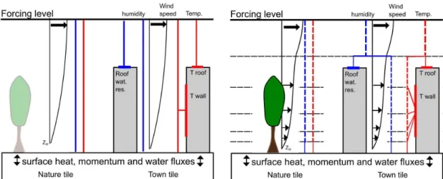
To improve the description of the physical coupling between the air and the surface, a one-dimensional surface boundary layer has been implemented in SURFEX in order to account for the vertical gradients of the variables of the lowest part of the atmosphere (Masson and Seity, 2009; Fig. 5). The main objectives of the use of an SBL in SURFEX are to
1. Better simulate the profile of wind, temperature, humid-ity and turbulence between the surface and the forcing level (usually, this is done diagnostically using Monin-Obuhkov similarity laws). This improves the forecast of near-surface air temperature at night when stability is strong (Masson and Seity, 2009).
2. Take account of the effect of vegetation or urban canopies on the in-canopy air. For example, it allows the micro-climate between buildings to be simulated in TEB, or the wind profile to be modified by the trees. For wind, it uses a drag force of the form du/dt= −Cd(z)u, whereuis the wind speed and where the drag coeffi-cient depends on building density or the leaf area index of trees. Heat and water fluxes directly influence the at-mospheric surface layer at the height where they are re-leased.
3. Better force the surface model, using air characteristics at the corresponding level (e.g. in TEB, near-road air temperature is used for roads, while mid-height canyon air temperature is used for walls).
One SBL profile is implemented for each of the four main tiles. First layers are usually at 50 cm, 2 m, 4 m, 7 m, and 10 m above the surface, but can be modified. Two metre tempera-ture and humidity, and 10 m wind, are prognostically com-puted by the SBL scheme for each tile. Note that the SBL scheme is implicitly coupled with the surface schemes, but not with the atmosphere, which may cause instabilities for long time steps. Hence, the SBL is not used for climate runs. 6.1.3 Orographic friction
Fig. 5.Schematic view of the coupling between the surface (ISBA and TEB) and the atmosphere without the SBL model(a)and with the SBL model(b). In the latter case, a drag force is applied in the Nature and Town tiles for the wind. The temperature profile in the SBL model is influenced by the road, wall and roof temperatures. The humidity profile is influenced by the road and roof humidities.
approaches have been widely used, even for large mountains (e.g. Wood and Mason, 1993; Georgelin et al., 1994). Re-cent works (Beljaars et al., 2004) have preferred to parame-terize orographic drag not only at the surface but throughout a certain height above it (adding a drag force directly in the wind equations of the lowest layers of atmospheric models). Thanks to the SBL scheme included in SURFEX, the latter option can now be used in the surface scheme itself.
The friction can be computed by a roughness length or di-rectional roughness length (mostly depending on the main subgrid-valley directions, Georgelin et al., 1994), or by us-ing Beljaars et al.’s (2004) approach, in which case an ad-ditional SBL scheme with only wind and turbulence needs to be added. Orographic friction is caused by obstacles of a much larger horizontal scale than trees or even buildings. Therefore, these frictions are computed separately (assuming that the processes are independent of each other): the friction of natural land surface, towns, water and sea surface are av-eraged, and then only orographic friction is added, in the fol-lowing way: (u∗(total)2=u∗(surface)2+u∗(orography)2).
This also has the advantage that low-level air temperature and humidity are consistent with the characteristics of the land cover below (including its own roughness).
6.2 Coupling with hydrology
The main function of river routing models (RRMs) is to con-vert runoff simulated by LSMs into river discharge. The rout-ing of runoff estimates from LSMs is important to model river flow from large river basins and to estimate freshwater inflow into the oceans. The coupling of SURFEX with RRMs appears to be a powerful tool for understanding the regional and global water cycles (Habets et al., 1999b; Decharme and
Douville, 2007; Alkama et al., 2010), predicting streamflow (Habets et al., 2004; Quintana Segu´ı et al., 2009; Thirel et al., 2010), and improving model parameterizations (Boone et al., 2004; Decharme et al., 2006, 2010, 2011; Decharme and Douville, 2006a).
At catchment scale, ISBA can be coupled with the hy-drodynamical TOPODYN model (Pellarin et al., 2002). Up to now, this coupling has been used to simulate flash-flood events, such as those that occur over Mediterranean basins of France (Vincendon et al., 2010; Bouilloud et al., 2010). The northwestern Mediterranean area is prone to severe rainy events, especially in autumn. High cumulative amounts of precipitation fall on small to medium catchments, which are characterised by steep slopes and short hydrological response times. Mediterranean flash-floods are thus essentially driven by Dunne runoff over saturated areas. According to the TOP-MODEL approach (Beven and Kirkby, 1979), the TOPO-DYN model is based on the lateral soil water transfer follow-ing the topographical information but also takes the spatial variability of rainfall over a given catchment into account.
this application, spatial resolutions of 1 km for ISBA and 50 m for TOPODYN were used.
At the regional scale, SURFEX will soon have replaced an older version of ISBA within the M´et´eo-France hydrom-eteorological system SAFRAN-ISBA-MODCOU (SIM, Ha-bets et al., 2008) over France. In this suite, SURFEX is fed by a mesoscale meteorological analysis (SAFRAN, Quintana Segu´ı et al., 2008) and feeds a distributed hydrological model over France (MODCOU). Decharme and Douville (2006a) have also shown that this system is an interesting tool to eval-uate new model versions such as the set of sub-grid parame-terizations described in Sect. 4.1.
Finally, SURFEX is coupled with the global TRIP RRMs in order to study the continental part of the global hydro-logical cycle (Decharme and Douville, 2007; Alkama et al., 2010) and/or to close the hydrological budget in the CNRM-GAME climate model (Voldoire et al., 2012). The original TRIP RRM was developed by Oki and Sud (1998) at the University of Tokyo. It is used at M´et´eo-France to convert the simulated runoff into river discharge using a global river channel network at 1◦
or 0.5◦
resolution. TRIP considers a surface river reservoir, a simple one-dimensional groundwa-ter reservoir and a variable stream flow velocity (Decharme et al., 2010). Decharme et al. (2008, 2012) developed inter-active coupling between SURFEX and TRIP to simulate sea-sonal flood events and to represent their impact on the con-tinental evapotranspiration and energy budget for large-scale applications and climate modelling. The flood dynamics is described by including a prognostic flood reservoir in the daily coupling between ISBA and TRIP. This reservoir is full when the water level exceeds the bank-full limit and vice-versa. Its dimension evolves dynamically according to the flood water mass and the sub-grid topography in a given grid-cell. The reservoir interacts with surrounding soil through in-filtration and with the overlying atmosphere through precipi-tation interception and free water surface evaporation.
7 Data assimilation
The initialization of the prognostic variables of the surface schemes is an important issue for short- and medium-range weather forecasts, particularly for quantities that evolve more slowly than atmospheric timescales (e.g. deep soil moisture and temperature, snow reservoir). Without a dedicated ini-tialization, spurious feedbacks can take place between the atmosphere and the surface, driving the soil variables into unrealistic states (Viterbo and Courtier, 1995). The best ini-tialization is obtained from data assimilation systems that merge observations and model short-range forecasts opti-mally. Monitoring of land surface fluxes can also be signifi-cantly improved when observations are assimilated in surface schemes (e.g. Reichle et al., 2007).
7.1 Optimal interpolation
A first data assimilation system based on local optimum in-terpolation (OI), originally proposed by Mahfouf (1991) and adapted to operational numerical weather prediction systems at M´et´eo-France (Giard and Bazile, 2000), ECMWF (Dou-ville et al., 2000) and CMC (B´elair et al., 2003), is available in SURFEX for the assimilation of screen-level observations from the surface network (e.g. SYNOP and METAR reports). The OI scheme allows soil moisture contents and soil temper-atures to be corrected through the knowledge of short-range forecasts errors in temperature and relative humidity at 2 m. Analytical OI coefficients have been derived from Monte-Carlo single column experiments in clear-sky situations and need to be reduced when near-surface atmospheric errors are not informative about errors in the soil variables.
7.2 Extended Kalman filter (EKF)
Although still used by a number of numerical weather ser-vices, the OI scheme has a number of known weaknesses, such as its lack of flexibility regarding the observation types to be assimilated (only screen-level temperature and rela-tive humidity) and the model variables to be initialized (only the two soil reservoirs of the ISBA version based on the force-restore method). For these reasons, a new surface as-similation scheme based on the EKF has been developed within SURFEX. This scheme compares favourably with the OI scheme for the assimilation of screen-level observations (Mahfouf et al., 2009). The “offline” version of SURFEX forced by atmospheric parameters above screen level (around 20 m in the surface boundary layer) can efficiently compute (reduced numerical cost) the Jacobian matrix of the observa-tion operator. Also, the capability of the EKF to assimilate satellite-derived superficial soil moisture products from the radiometer AMSR-E/Aqua has been demonstrated (Draper et al., 2009). The combined assimilation of satellite-derived soil moisture and screen-level observations with the EKF was examined by Draper et al. (2011b). A simplified version of the SURFEX EKF using analytical Jacobians of the ISBA scheme has also been developed in order to examine the im-pact of satellite-derived soil moisture from the scatterometer ASCAT on numerical weather predictions (Mahfouf, 2010). Recently, Mahfouf and Bliznak (2011) proposed a method to efficiently combine information coming from precipitation analyses (radars or raingauges) and from screen-level mea-surements within the EKF.
of the ISBA-Ags model has allowed the Jacobians of a new variable, the vegetation biomass, to be examined (R¨udiger et al., 2010), and also the formulation of the EKF to be extended to the availability of 12 patches in a grid box (i.e. different surface and soil prognostic variables for each patch) and one single “grid-averaged” observation. Draper et al. (2011a) showed that the assimilation of the satellite-derived ASCAT soil moisture improve runoff and river dis-charge simulations when assimilated in the hydrometeoro-logical model SIM (Habets et al., 2008) using the SURFEX EKF data assimilation system. It must be noted that some products such as LAI and soil moisture are biased and re-quire a pre-processing, as SURFEX assumes that observa-tions are unbiased. For the present applicaobserva-tions, the biases are corrected using a “CDF (cumulative distribution func-tion) matching technique” (Reichle and Koster, 2004).
Finally, studies are currently under way to improve the specification of the covariance matrix of background errors in the EKF through a better description of model errors. Us-ing a model error term derived from an ensemble of short-range forecasts of precipitation, which is cycled through the filter, generates realistic spatial variability patterns in the background errors.
8 Model applications and evaluations
Most pre-existing scientific models (e.g. ISBA and TEB) were used and validated in various configurations before the building of SURFEX, both in offline mode and coupled with the atmosphere. As an example, ISBA (Noilhan and Planton, 1989) has been regularly improved over more than 20 yr. The scientific work of improvement and validation of the physics continued during the transition from the pre-existing codes to SURFEX while, from a technical point of view, the progres-sive replacement of the surface components implied signifi-cant technical work. In most cases, the introduction of SUR-FEX into the applications (in particular atmospheric models) allowed an improvement of the surface parameterization and scores, drawing benefit from the use of an up to date exter-nalized surface scheme.
It is beyond the scope of this paper to provide a compre-hensive review of all the validations of the sub-models in-cluded in SURFEX. In the first sub-section, the applications and validations in offline mode (either local or distributed) will be reviewed rapidly. Then, the impact of the introduc-tion of SURFEX in atmospheric models will be shown. 8.1 Applications in offline mode
8.1.1 ISBA
The original version of ISBA (Noilhan and Planton, 1989) and further improved versions have been extensively vali-dated against measurements at the local scale and
partici-pated in many intercomparison projects that have stimulated improvements in the model:
– PILPS (Henderson-Sellers et al., 1993): ISBA applica-tion to the Cabaw (Chen et al., 1997), and Arkansas River (Wood et al., 1998; Liang et al., 1998; Lohmann et al., 1998) datasets, leading to improved subgrid hy-drology. The simulation of a Scandinavian basin (Ha-bets et al., 2003) was the first application of the multi-layer soil option of ISBA for hydrology and validated the cold processes in the soil. Valda¨ı (Slater et al., 2001 and Luo et al., 2003) was the occasion to further validate the snow and cold processes in the soil.
– GSWP (Dirmeyer et al., 1999, 2006): validation and in-tercomparison of hydrological parameterization at the global scale, including uncertainties associated with the forcing data (Decharme and Douville, 2006b).
– Rhone-Aggreg (Boone et al., 2004): testbed for scale changes, subgrid hydrology and the use of the multi-layer snow model (ISBA-ES).
– SnowMIP (Etchevers et al., 2003; Rutter et al., 2009): importance of the representation of albedo in snowpack models, simulation of the liquid water content in the snow for an accurate prediction of snowmelt, impor-tance of the interaction between snow and vegetation for an accurate simulation of the snow cover in forests. More recently, SURFEX has been applied in Africa within ALMIP (AMMA Land Surface Models Intercomparison Project; Boone et al., 2009), a validation of the surface en-ergy budget over France using different sources for the in-coming solar radiation, including METEOSAT satellite esti-mates, has been undertaken by Carrer et al. (2012) and the multilayer soil scheme (Boone et al., 2000) has been exten-sively validated by Decharme et al. (2011) at the SMOSREX (Surface Monitoring Of Soil Reservoir Experiment) site in the south west of France.