ILDIKÓ KNEISZ
1ABSTRACT - The paper presents how economic structural changes affect a region’s economic growth
and development. To show this effect is not that easy since changes of economic structure take time, and the result of changes appear shifted in time in the examined regions. Researchers examining reasons of income disparities among countries pay attention to the question how differences of GDP levels and growth rates can be explained by the economic structures. Literature of economic development sets store by explanatory potential of differences in macro-structures in countries within especially for share of agriculture in gross domestic product.
Keywords: regional development, territorial disparities, sectoral analysis, shift-share analysis.
INTRODUCTION
Several studies (e.g. European Commission 2001; European Commission 2004; Petrakos, 2000) confirm that throughout the last decade, the accession countries witnessed increasing regional disparities. In its latest report on economic and social cohesion, the European Commission (2004) finds that economic growth in the CEECs has not been regionally balanced.
Growing empirical evidence (e.g. Bachtler et al. 1999; European Commission 2001; Petrakos, 2000; Resmini, 2002) points to one type of winner and to two types of losers among the accession countries’ regions: in this admittedly simplified dichotomy, the metropolitan and urban areas (namely the capital city regions) belong to the former group, the rural and old (declining) industrial areas as well as those in the Eastern peripheries belong to the latter group.
According to Lıcsei (2004), on national and international level, it is confirmed that, since the
industrial revolution, between economic state of development and macroeconomic structure – from the point of view of production and employment – is a strong connection. Statically (cross-sectional) and dynamically (time series), it can be set out that by economic development the share of agriculture is decreasing in employment, as well as in economic value added, and the share of industry and services is increasing.
Regions’ economy can be traditionally structured into three sectors. In the primary sector (agriculture, hunting, forestry and fishing), the lands as capital goods have basically a determining role; in the secondary sector (industry and manufacture), processing and transformation are stressed on, while the tertiary sector (services) has human resources as function.
In this study, we try to find out whether development differences are caused by regional position or by economic structure. All indicators are calculated at NUTS 2 level. Main indicators are regional GDP and employment in the examined regions of Romania and Hungary and all the sources of indicators are Eurostat electronic and printed database.
Recent development path in Romania is determined by economic-social transformation, new political and economic condition after the change. Economic development is mainly defined, not exactly by sectoral transformations, but by enterprises’ competitiveness at micro level (Illés, 2002).
In the 90s, economic growth in Romania has declined to the deepest (in 1990, national economic growth: –7.4%; in 1994, it takes 1%), while stabilization of economic change was hold up by high inflation and foreign debt. Distinct improvement has came around 2000, where in 2001 growth in GDP per capita has reached even 5.7% which was an outcome of quantity flare of economic activities mainly in the trade, merchandise and construction sectors.
1 Assistant Lecturer, University of Miskolc, Faculty of Economics, Institute of World and Regional Economics,
ILDIKÓ KNEISZ
8
0 20 40 60 80
Nord-Vest
Centru
Nord-Est
Sud-Est
Sud - Muntenia Bucuresti - Ilfov
Sud-Vest Oltenia Vest
2000 2005
0 20 40 60 80 100 120
Közép-Magyarország
Közép-Dunántúl
Nyugat-Dunántúl
Dél-Dunántúl Észak-Magyarország
Észak-Alföld Dél-Alföld
1995 2000 2005
Romania Hungary
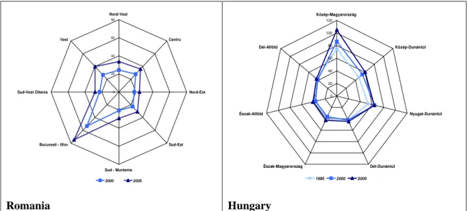
Figure 1. Regional GDP in EU percentage (1995, 2000, 2005).
(Source: Own compilation on Eurostat database)
Industrial employment in Romania fell down in the 90s from 34% to 27% until 2000 and rest of the active population turned to self-sufficient agriculture or, a small part of them, to some service branches. Therefore, a strong employment growth in the primary sector took place in Romania, which led to a huge rural population.
0% 10% 20% 30% 40% 50% 60% 70% 80% 90% 100%
1999 2000 2001 2002 2003 2004 2005 2006
agriculture industry services
Hungary
0% 10% 20% 30% 40% 50% 60% 70% 80% 90% 100%
1999 2000 2001 2002 2003 2004 2005 2006
agriculture industry services
Romania
Figure 2. National employment rates in the examined two countries, 1999-2006 (%).
(Source: Own compilation on Eurostat database)
2000 2001 2002 2003 2004 2005
1. Bucuresti -
Ilfov 24.7 Vest 8.8
Central
Hungary 8.0
Sud-Vest
Oltenia 11.1 Sud-Est 15.2
Bucuresti - Ilfov
14.6
2. Central
Transdanubia 9.1
Northern
Great Plain 8.5 Centru 7.6 Vest 9.6
Sud -
Muntenia 11.7
Central
Hungary 8.2
3. Central
Hungary 6.0
Bucuresti -
Ilfov 8.4 Nord-Vest 7.1
Central
Transdanubia 9.5 Vest 9.7 Nord-Est 3.4
4. Western
Transdanubia 5.6 Nord-Est 8.3
Sud -
Muntenia 6.4
Western
Transdanubia 9.4 Nord-Vest 8.6
Central
Transdanubia 3.0
5. Northern
Great Plain 5.2
Sud -
Muntenia 6.2 Vest 6.3 Nord-Vest 8.1
Northern
Hungary 8.3
Sud -
Muntenia 2.9
6. Northern
Hungary 2.8 Central Hungary 5.5 Nord-Est 5.8 Sud - Muntenia 6.6 Southern Great Plain 7.7 Vest 2.2
7. Southern
Great Plain 2.6
Northern
Hungary 5.0 Sud-Est 5.5
Northern
Great Plain 5.8
Sud-Vest
Oltenia 7.5 Nord-Vest 2.1
8. Centru 2.2 Nord-Vest 4.8 Western
Transdanubia 3.2 Centru 5.6
Central
Transdanubia 7.1
Northern
Hungary 1.7
9. Southern
Transdanubia 1.1
Southern
Transdanubia 4.3
Bucuresti -
Ilfov 2.7 Nord-Est 5.5
Bucuresti -
Ilfov 6.9 Sud-Est 1.3
10. Nord-Vest -0.9 Sud-Est 3.0 Northern
Hungary 2.7
Northern
Hungary 4.7 Centru 5.3 Centru 1.3
11. Sud-Vest
Oltenia -1.8 Centru 2.8
Southern
Great Plain 2.3 Sud-Est 4.6
Northern
Great Plain 5.0
Southern
Transdanubia 1.1
12. Sud-Est -2.7 Southern
Great Plain 2.5
Southern
Transdanubia 2.2
Southern
Great Plain 2.4
Southern
Transdanubia 4.7
Southern
Great Plain 1.0
13. Nord-Est -2.8 Central
Transdanubia 2.1
Northern
Great Plain 1.4
Central
Hungary 2.1 Nord-Est 4.1
Northern
Great Plain 0.3
14. Sud -
Muntenia -3.9
Sud-Vest
Oltenia 1.5
Sud-Vest
Oltenia 0.3
Southern
Transdanubia 1.8
Central
Hungary 4.0
Western
Transdanubia -1.1
15. Vest -8.5 Western
Transdanubia -2.8
Central
Transdanubia -1.9
Bucuresti -
Ilfov -1.7
Western
Transdanubia 0.9
Sud-Vest
Oltenia -2.4
ILDIKÓ KNEISZ
10
The higher employment in agriculture is shown in the Romanian regions except for the capital region, Bucharest (no. 80), with a rate under 3%. The highest values are in the Nord-Est (no. 58) and in the Sud-Vest Oltenia (no. 82) regions. A low economic performance, between 22% and 40% in GDP in EU-average, is connected to the high agricultural employment.
120,00 100,00 80,00 60,00 40,00 20,00
GDP in EU-average (%) 2005 0,50 0,40 0,30 0,20 0,10 0,00 E m p lo y m e n t ra te ( A ,B ) 2 0 0 5 88 82 80 72 65 58 51 44 39 35 31 27 23 19 17 Romania Hungary Country 120,00 100,00 80,00 60,00 40,00 20,00
GDP in EU-average (%) 2005 0,50 0,40 0,30 0,20 0,10 0,00 E m p lo y m e n t ra te ( C ,D ,E ) 2 0 0 5 88 82 80 72 65 58 51 44 39 35 31 27 23 19 17 Romania Hungary County
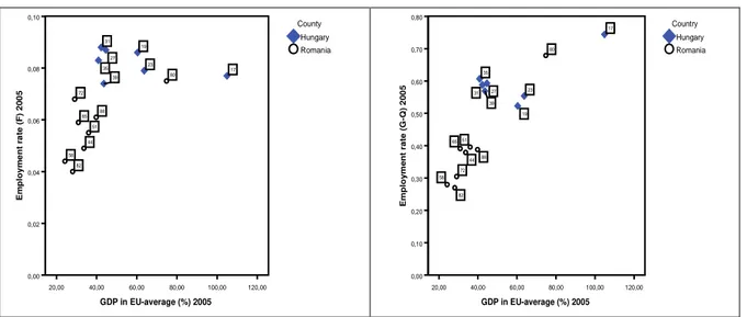
Figure 3. Regional employment rate compared to regional GDP in selected sectors (2005).
(Source: Own compilation on Eurostat database)
All Hungarian regions perform above 40% in GDP in EU-average but with a significant lower rate of employment in agriculture. It means that the domestic value added comes in Hungary not from agriculture. Industrial employment is in both counties’ regions between 18% and 38%. It is shown that this branches (mining and quarying; electricity, gas and water supply) gives the second larges part of regional employments. In Hungary this high rate appears in Central Transdanubia (nr. 19) and Western Transdanubia (nr. 23) while in Romania the Central region (nr. 51) and Western region (nr. 88).
120,00 100,00 80,00 60,00 40,00 20,00
GDP in EU-average (%) 2005
0,10 0,08 0,06 0,04 0,02 0,00 E m p lo y m e n t ra te ( F ) 2 0 0 5 88 82 80 72 65 58 51 44 39 35 31 27 23 19 17 Romania Hungary County 120,00 100,00 80,00 60,00 40,00 20,00
GDP in EU-average (%) 2005
0,80 0,70 0,60 0,50 0,40 0,30 0,20 0,10 0,00 E m p lo y m e n t ra te ( G -Q ) 2 0 0 5 88 82 80 72 65 58 51 44 39 35
31 27 23
19
17
Romania Hungary Country
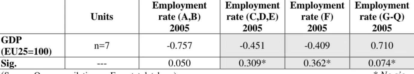
Figure 4. Regional employment rate compared to regional GDP in selected sectors (2005).
(Source: Own compilation on Eurostat database)
Another point of view indicates that the capital city and the biggest cities have the better employment potential, due to the presence of larger companies. The small cities and other settlements have a high rate of micro and small enterprises, which have a lower employment potential.
A connection between employment rate and regional economic performance correlate, in the case of Hungary, only in agriculture, but it is a negative one. Therefore, when agricultural employment declines, economic performance should get even higher, as industrial and service sector value added gets higher.
Table 2. Correlation between GDP and sectoral2 employment in Hungary.
Units
Employment rate (A,B)
2005
Employment rate (C,D,E)
2005
Employment rate (F)
2005
Employment rate (G-Q)
2005 GDP
(EU25=100) n=7 -0.757 -0.451 -0.409 0.710
Sig. --- 0.050 0.309* 0.362* 0.074*
(Source: Own compilation on Eurostat database) * No sig.
The analysis of the 8 Romanian regions has shown that the primary and tertiary sectors have strong connection to regional economic performance. In case of agriculture, the same negative correlation appears, but in the service sector the positive relation is typical.
Table 3. Correlation between GDP and sectoral employment in Romania.
Units
Employment rate (A,B)
2005
Employment rate (C,D,E)
2005
Employment rate (F)
2005
Employment rate (G-Q)
2005 GDP
(EU25=100) n=8 -0.882 0.113 0.706 0.972
Sig. --- 0.004 0.789* 0.050* 0.000
(Source: Own compilation on Eurostat database) * No sig.
METHODOLOGY AND DATA
In case of economic structure, the analysis of the different approaches belongs to different method backgrounds. In most cases, simple and complex quantitative methods are applied. In regional researches, we can use two ways of solving measurement problems. One could be the simplification manner, by selecting one or only a few indicators and analysing them. The other possibility is to choose a wider view and analyse many indicators as a whole (Rechnitzer ed., 1994).
Shift-share analysis is a method of decomposing regional income or employment growth patterns into expected (share) and differential (shift) components. The description of the economy provided by shift-share can be used in the research that explores the reasons for change. It is strictly a descriptive technique. By itself, it cannot be used to elicit the determinant economic trends.
The technique was first applied in the U.S. to calculate employment change from 1939 to 1954 (Dunn, 1960). Its origins date from the 1940's when an economist working for the U.S. Bureau of Labour and Statistics developed the concept of "location shifts" used to measure growth trend differences between the nation and its states (Cramer, 1942). Shift-share is utilized by regional
2Analysed sectors: A, B (Agriculture, hunting, forestry and fishing); C, D, E (Mining and quarrying; electricity,
ILDIKÓ KNEISZ
12
economists, community planners, and policy analysts to provide quick sketches of the economic landscape of both rural and urban areas.
Shift-share analysis decomposes regional growth into separate and unique factors influencing the prosperity of spatially distinct areas. Most shift-share models are mathematical identities expressing economic upswings (or downturns) as a function of three broad factors: the national growth effect, the industrial mix effect, and the competitive effect. Between any two time periods, the observed change in growth is assumed to be the sum of these three effects or components.
The classic shift-share model is defined as:
Etij - Et-1ij = ∆ Eij = NEij + IMij + CEij
Etij = Employment (income) in the ith sector in the jth region at time t
NEij = National Growth Effect
IMij = Industrial Mix Effect
CEij = Competitive Effect
National Growth Effect
The national growth effect is the amount that total regional employment would have grown if it grew at precisely the same rate as total employment in the nation as a whole. Implicitly, the model asserts that the industries in a region will grow at approximately the rate of national industries unless the region has a comparative advantage or disadvantage.
Industry Mix
Most regions do not have identical industrial profiles. Some regions are home to a preponderance of slow-growing sectors, while others may specialize in sectors with growth rates that are higher than the national average. The industry mix effect in the shift-share equation tries to capture these regional variations in industrial composition. The industry mix is the amount of growth attributable to differences in the sectoral makeup of the region versus that of the nation.
Both the national growth effect and the industry mix effect are exogenous factors that are determined by national growth rates, not local or regional economic conditions. Together, they comprise the region's expected growth - the growth that would occur in the region if each of the industries grew at the same rate as the nation as a whole.
Competitive Effect
The competitive effect is a "shift" from what would be expected if the region's industry grew at exactly the proportion of national growth and industry mix. Implicit in shift-share analysis is the assumption that regional economies should grow at national growth rates unless there are comparative advantages or disadvantages operating at the regional level.
The growth attributed to the competitive effect is the value that is left after the national growth effect and industry mix are subtracted. This residual is inferred to result from factors that are unique to the region. The competitive effect arises from interregional differences affecting a given area's attractiveness to the activity. These differences develop because of endogenous factors inherent to the region. The competitive effect can be thought of as a measurement of a region's competitive edge or
comparative advantage in the production of the goods in the ith industry.
Applicability of shift-share method (Kalocsai and López, 2005):
− Analysis of structure of branches
− Merchandise and market analysis
− Migration analysis
− Analysis of regional growth (neoclassic point of view)
− Forecasting (economic growth, population)
− Regional specialisation
We analysed 15 regions in Hungary and Romania. Hungarian regions are in better situation compared to most of the Romanian regions, which can be confirmed by static indicators. But most of the dynamic indicators prove the significant improvement of the Romanian regions in economic terms.
RESULTS
Four regions – three Hungarian and one Romanian (Southern Great Plain, Southern Transdanubia, Western Transdanubia, Sud-Vest Oltenia) – have an absolutely disadvantaged position, while the unfavourable structural effects are strengthened by the worse employment potentials. It is very interesting that only the Hungarian central region shows lower employment decline among the 15 regions.
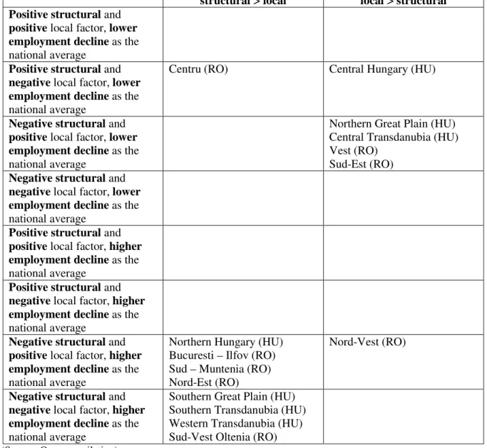
Table 4. Role of local and structural effects in the employment rate changes in
Hungarian and Romanian regions (2000-2006).
structural > local local > structural
Positive structural and
positive local factor, lower
employment decline as the
national average
Positive structural and
negative local factor, lower
employment decline as the
national average
Centru (RO) Central Hungary (HU)
Negative structural and
positive local factor, lower
employment decline as the
national average
Northern Great Plain (HU) Central Transdanubia (HU) Vest (RO)
Sud-Est (RO)
Negative structural and
negative local factor, lower
employment decline as the
national average
Positive structural and
positive local factor, higher
employment decline as the
national average
Positive structural and
negative local factor, higher
employment decline as the
national average
Negative structural and
positive local factor, higher
employment decline as the
national average
Northern Hungary (HU) Bucuresti – Ilfov (RO) Sud – Muntenia (RO) Nord-Est (RO)
Nord-Vest (RO)
Negative structural and
negative local factor, higher
employment decline as the
national average
Southern Great Plain (HU) Southern Transdanubia (HU) Western Transdanubia (HU) Sud-Vest Oltenia (RO)
(Source: Own compilation)
ILDIKÓ KNEISZ
14
speaking, Budapest and Hungary’s Western parts are characterised by good infrastructure links (e.g. the M1 motorway), by a dynamically growing private sector activity and by a great number of international joint ventures which act as connections to international networks (Bachtler et al., 1999). While Budapest has attracted basically tertiary activities (mainly financial services), the counties of
Gyır-Moson-Sopron and Vas have become centres of specialised industrial mass-production
(Rechnitzer, 2000).
The Eastern periphery (the counties of Szabolcs-Szatmár-Bereg and Hajdú-Bihar) suffers from a regional crisis in the manufacturing and agricultural industries, which were producing for the Soviet market: three Eastern Hungarian industrial counties account for around 35 per cent of the country’s total unqualified and unemployed workers. The employment power of the weak service sector is still far too low to absorb those who lost their jobs due to the systemic change.
Generally, Hungary’s Southern, Northern and (North-) Eastern counties have comparatively poor infrastructure connections, small numbers of joint ventures and a very weak private sector (Bachtler et al. 1999). Among other factors, it is the lack of favourable transport connections that makes regions like North-East Hungary and the Great Hungarian Plain far less competitive (Rechnitzer, 2000). Hungary’s Southern, Northern and (North-) Eastern border regions are all peripheries, their economic sources and potential are still moderate and limited (Rechnitzer, 2000).
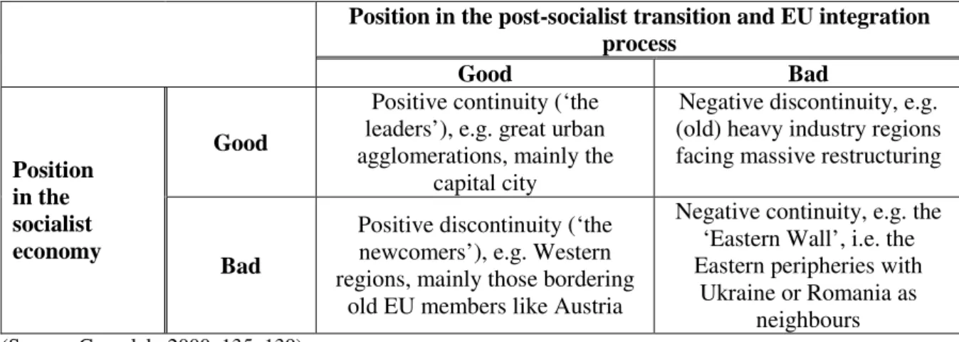
Table 5.Position in the socialist economy and in the post-socialist transition
and EU integration process.
Position in the post-socialist transition and EU integration process
Good Bad
Good
Positive continuity (‘the leaders’), e.g. great urban agglomerations, mainly the
capital city
Negative discontinuity, e.g. (old) heavy industry regions facing massive restructuring Position
in the socialist economy
Bad
Positive discontinuity (‘the newcomers’), e.g. Western regions, mainly those bordering
old EU members like Austria
Negative continuity, e.g. the ‘Eastern Wall’, i.e. the Eastern peripheries with
Ukraine or Romania as neighbours
(Source: Gorzelak, 2000, 135–139)
CONCLUSIONS
REFERENCES
BACHTLER, J., R. DOWNES, E. HELIOSKA-HUGHES, AND J. MACQUARKIE. (1999),
Regional development and policy in the transition countries. Regional and Industrial Policy Research Paper 36. European Policies Research Centre, Glasgow.
CRAMER, D. (1942), Shifts of Manufacturing Industries, Industrial Location and Natural
Resources. U.S. Government Printing Office, Washington, D.C.
DUNN, E. S. (1960), A statistical and analytical technique for regional analysis. Papers of the
Regional Science Association Vol.6, 97-112.o.
EUROPEAN COMMISSION (2001), Real convergence in candidate countries: Past performance
and scenarios in the pre-accession economic programmes. ECFIN/708/01-EN.
EUROPEAN COMMISSION (2004), Third Report on economic and social cohesion.
Luxembourg: Office for Official Publications of the European Communities.
GORZELAK, G. (2000), The dilemmas of regional policy in the transition countries and the
territorial organisation of the state. In: Integration and transition in Europe: The
economic geography of interaction, eds. G. Petrakos, G. Mayer, and G. Gorzelak, 131–49.
London: Routledge.
ILLÉS, I.(2002), Közép- és Délkelet-Európa az ezredfordulón, Dialóg–Campus Kiadó, Budapest–
Pécs.
KALOCSAI, K., LÓPEZ, A. J. (2005), Predicción del efecto de la UE en Hungría del Norte.
Análisis comparativo con Asturias. Hispalink-Asturias, 2/2005 Documento, AS-6139-2005, Oviedo.
KOCZISZKY, GY. (2003), Economic growth in Hungary 1990-2000. RSA International 33. rd.
Annued Conference. University of St. Andrews, Scotland (co-writer: Dr. Bakos István).
KOCZISZKY, GY. (2006), Versenyképességi elemek a hazai regionális stratégiákban. (In:
Horváth Gyula (szerk.): Régiók és települések versenyképessége. MTA Regionális Kutatások Központja. Pécs, pp. 443-462.
KOCZISZKY, GY. (2006), Az Észak-magyarországi régió felzárkózási esélyei.
Észak-magyarországi Stratégiai Füzetek III. évf. 2006/1. pp. 128-147.
LACKENBAUER, J. (2004.), Catching-up, Regional Disparities and EU Cohesion Policy: The
Case of Hungary. In Managing Global Transitions (Edited by Bostjan Antoncic), 2004, vol. 2, issue 2, pages 123-162.
LIIKANEN, E. (1999), Strukturwandel und Anpassungsleistungen im europäischen
verarbeitenden Gewerbe. Mitteilung der Kommission an den Rat, das Europäische Parlament, den Ausschuß der Regionen und den Wirtschafts- und Sozialausschuß.
LİCSEI, H. (2004), A foglalkoztatás ágazati és regionális dimenzióinak kapcsolata az ezredvégi
Magyarországon. Regionális Tudományi Tanulmányok, 9. kötet, Az ELTE Regionális Földrajzi Tanszék és az MTA-ELTE Regionális Tudományi Kutatócsoport
kiadványsorozata, Sorozatszerkesztı: Nemes Nagy József.
NEMES NAGY, J. (1987), A regionális gazdasági fejlıdés összehasonlító vizsgálata. Akadémiai
Kiadó, Budapest.
PETRAKOS, G. (2000), The spatial impact of East-West integration. Integration and transition in
Europe: The economic geography of interaction, eds. G. Petrakos, G.Mayer, and
G.Gorzelak, 38–68. London: Routledge.
RECHNITZER, J. (1994) (szerk.), Fejezetek a regionális gazdaságtan tanulmányozásához. MTA
ILDIKÓ KNEISZ
16
RECHNITZER, J. (2000), The features of the transition of Hungary’s regional system. Discussion
Paper 32. Centre for Regional Studies of the Hungarian Academy of Sciences, Pécs.
RESMINI, L. (2002), Specialization and growth prospects in border regions of accession