www.biogeosciences.net/10/6721/2013/ doi:10.5194/bg-10-6721-2013
© Author(s) 2013. CC Attribution 3.0 License.
Biogeosciences
Seasonal dissolved inorganic nitrogen and phosphorus budgets for
two sub-tropical estuaries in south Florida, USA
C. Buzzelli1, Y. Wan1, P. H. Doering1, and J. N. Boyer2
1Coastal Ecosystems Section, South Florida Water Management District, West Palm Beach, Florida 33406, USA 2Center for the Environment and Department of Environmental Science and Policy, Plymouth State University, 17 High
Street, MSC #63, Plymouth, New Hampshire 03264, USA
Correspondence to:C. Buzzelli (cbuzzell@SFWMD.gov)
Received: 3 January 2013 – Published in Biogeosciences Discuss.: 11 February 2013 Revised: 18 September 2013 – Accepted: 25 September 2013 – Published: 24 October 2013
Abstract. Interactions among geomorphology, circulation, and biogeochemical cycling determine estuary responses to external nutrient loading. In order to better manage water-shed nutrient inputs, the goal of this study was to develop seasonal dissolved inorganic nitrogen (DIN) and phospho-rus (DIP) budgets for the two estuaries in south Florida, the Caloosahatchee River estuary (CRE) and the St. Lucie Estu-ary (SLE), from 2002 to 2008. The Land–Ocean Interactions in the Coastal Zone (LOICZ) approach was used to generate water, salt, and DIN and DIP budgets. Results suggested that internal DIN production increases with increased DIN load-ing to the CRE in the wet season. There were hydrodynamic effects as water column concentrations and ecosystem nutri-ent processing stabilized in both estuaries as flushing time in-creased to>10 d. The CRE demonstrated heterotrophy (net ecosystem metabolism or NEM<0.0) across all wet and dry season budgets. While the SLE was sensitive to DIN load-ing, system autotrophy (NEM>0.0) increased significantly with external DIP loading. This included DIP consumption and a bloom of a cyanobacterium (Microcystis aeruginosa) following hurricane-induced discharge to the SLE in 2005. Additionally, while denitrification provided a microbially-mediated N loss pathway for the CRE, this potential was not evident for the SLE where N2fixation was favored.
Dispari-ties between total and inorganic loading ratios suggested that the role of dissolved organic nitrogen (DON) should be as-sessed for both estuaries. Nutrient budgets indicated that net internal production or consumption of DIN and DIP fluctu-ated with inter- and intra-annual variations in freshwater in-flow, hydrodynamic flushing, and primary production. The results of this study should be included in watershed
man-agement plans in order to maintain favorable conditions of external loading relative to internal material cycling in both dry and wet seasons.
1 Introduction
S-79
Sanibel PI-01
38-3GR 39-20GR
26-3GR20 25-3GR20 24-7GR 23-5GR
18-6GR
16-3GR
20-9GR 20A-11GR 22-7GR
21-7GR
CES02
CES04
CES05
CES06
CES07 CES08
CES09
Upstream flow
Tributary flow & WQ
Estuary WQ
Downstream WQ
Downstream salinity
Fig. 1.Map depicting the Caloosahatchee River estuary. See Table 1 and Sect. 2.2 for details of data sources and integration into the nutrient budgets. Included is the upstream boundary site of gauged freshwater inflow (S-79; filled star), 12 locations of tributary water quality data (open circles), 7 locations of estuary water quality data (open squares), the location of downstream water quality data (PI-01; open cross), and the downstream boundary location for salinity (Sanibel; open star).
Baseline quantification of material inputs, flushing time, downstream export, and the potential for internal production or consumption of C, N, and P (CNP) is essential to better un-derstand estuarine system metabolism (Gordon et al., 1996; Smith et la., 2005; Giordani et al., 2008). This is particularly true for coastal water bodies with heavily managed freshwa-ter inflow subject to both short- and long-freshwa-term fluctuations in discharge (Brock, 2001). In fact, sensitivity to both re-duced inflows (loss of freshwater and estuarine habitats) and increased inorganic nutrient loading (symptoms of eutroph-ication) offers an apparent contradiction for estuarine man-agement (Flemer and Champ, 2006). The amount of water and dissolved materials required to maintain optimal system metabolism with regard to CNP production and consumption should be quantified and factored into management plans for coastal watersheds.
In 1993 the International Geosphere-Biosphere Program (IGBP) and the International Human Dimensions Program on Global Environmental Change (IHDP; http://www.loicz. org/; http://nest.su.se/mnode/) initiated a project to inves-tigate biogeochemistry of the coastal zone (Gordon et al., 1996; Smith et al., 2005; Swaney et al., 2011). The Land– Ocean Interactions in the Coastal Zone (LOICZ) included a spreadsheet tool designed to quantify internal C, N, and P sources and sinks in estuaries (Giordani et al., 2008). LOICZ also has been useful in socio-economic-political assessments
of human dimensions in the coastal zone (Talaue-McManus et al., 2003; Swaney et al., 2011). The approach has been used to investigate CNP cycling in hundreds of coastal en-vironments (Smith et al., 2005; Giordani et al., 2008; Ya-mamoto et al., 2008; Liu et al., 2009; Swaney et al., 2011. The spreadsheets are customizable depending upon the qual-ity and quantqual-ity of data and can be applied to any estuary without the need for detailed rate process information.
2 Methods
2.1 Study sites
The CRE is located in southwest Florida and has been al-tered by human activities starting in the 1880s when the river was straightened and deepened (Fig. 1; Antonini et al., 2002). The first water control structures at Lake Okeechobee (S-77) and Ortona (S-78) were completed in the 1930s with the last installed in 1966 at Olga (S-79; Antonini et al., 2002). The Franklin Lock at S-79 represents the head of the CRE that extends∼42 km downstream to Shell Point where it empties into the Gulf of Mexico. The meso- and poly-haline estuary downstream of S-79 has also experienced anthropogenic im-pacts (Chamberlain and Doering, 1998). Early descriptions of the CRE characterize it as barely navigable due to exten-sive shoals and oyster bars near the estuary’s mouth (Sackett, 1888). A navigation channel was dredged with a causeway built across the mouth of San Carlos Bay in the 1960s. His-toric oyster bars immediately upstream were mined for road construction.
Located in southeast Florida, the SLE comprises a major tributary to the ecologically and commercially valuable In-dian River lagoon (Sime, 2005; Ji et al., 2007; Fig. 2). Histor-ically, the SLE was a freshwater system that was temporarily exposed to the coastal ocean only through ephemeral inlets (United States Army, 1915). The St. Lucie Inlet was perma-nently opened in 1892 to provide a connection between the SLE and coastal ocean resulting in a partially mixed estu-ary with semi-diurnal tidal amplitude of∼0.4 m. The past several decades have seen the SLE watershed altered from a system of natural sloughs and wetlands into a series of sub-basins affected by agriculture and urbanization. The SLE has a large watershed : estuary surface area ratio of 150:1 (Tampa Bay, 5.5:1). Watershed changes and periodic high-volume water releases from Lake Okeechobee have altered historical wet season and dry season patterns of nutrient load-ing. These changes in flow, salinity, and water quality are as-sociated with increased prevalence of phytoplankton blooms, accumulation of muck-like sediments, and the loss of sea-grass and oyster habitats (Sime, 2005; SFWMD, 2012a).
2.2 Application of the LOICZ approach to the Caloosahatchee and St. Lucie estuaries
Application of the LOICZ approach results in water, salt, DIN, and DIP budgets for the estuary of interest (Gordon et al., 1996; Smith et al., 2005; Giordani et al., 2008; Swaney et al., 2011; the reader is encouraged to refer to these pub-lished efforts for conceptual and mathematical details of the LOICZ approach). It was designed to isolate internal, non-conservative production or consumption of dissolved CNP from conservative exchanges for a spatially homogeneous layer, segment, or estuarine water body.
Gordy
C-24; S-49
C-23; S-48
C-44; S-80 HR1
SE03 SE02
SE01
SE11
SE04
Upstream flow
Tributary flow & WQ
Estuary WQ Downstream salinity & WQ
Fig. 2. Map depicting the St. Lucie Estuary. See Table 1 and Sect. 2.2 for details of data sources and integration into the nutrient budgets. Included is the upstream boundary for freshwater inflow (Gordy Rd.; filled star), three locations of tributary water quality and inflow data (open circles), six locations of estuary water qual-ity data (open squares), and the downstream boundary location for water quality and salinity (SE-11; open star).
The approach assumes a steady state condition that bal-ances the sum of physical inputs against the sum of phys-ical outputs (Wosten et al., 2003; Swaney et al., 2011). In general, salinity (S) differences between the estuary and the downstream oceanic boundary are used to define net flows, residual exchange, and flushing time (Tf). The water budget
and hydrodynamic exchange attributes are used to predict in-ternal production or consumption of dissolved inorganic C, N, and P. This study generated budgets in order to evaluate net internal production or consumption of DIN (1 DIN; g N m−2d−1)and DIP (1DIP; g P m−2d−1)at the seasonal
Table 1.Sources of input data for seasonal DIN and DIP budgets for CRE and SLE. Please see Sect. 2.2 for explanation and details and Figs. 1 and 2 for water quantity and quality monitoring locations.
Abbreviation Definition Unit CRE SLE
Vrain Rain to estuary surface 106m3d−1 Nexrad Nexrad
VQ Freshwater discharge 106m3d−1 DBHydro S-79 DBHydro S484980+Gordy
VOFW Tributaries+groundwater 106m3d−1 Tidal basin model 30 % of total Q
Ve Estuary volume 106m3 Interpolated bathymetry Interpolated bathymetry
Se Estuary salinity DBHydro CES stations DBHydro SE stations
So Downstream bound salinity Shell Point daily model DBHydro station SE-11
DIPrain DIP in rain g m−3 DBHydro averages DBHydro averages
DIPQc DIP in discharge g m−3 Lee County Stations DBHydro S-484980
DIPOFW DIP in tributaries+gw g m−3 Lee County Stations DBHydro S-484980
DIPe DIP in estuary g m−3 DBHydro CES stations DBHydro SE stations
DIPo DIP in downstream bound g m−3 Lee County Stn. PI-01 DBHydro station SE-11
DINrain DIN in rain g m−3 NADP St. Petersburg, FL NADP St. Petersburg, FL
DINQc DIN in discharge g m−3 DBHydro station S-79 DBHydro S-484980
DINOFW DIN in tributaries+gw g m−3 Lee County Stations DBHydro S-484980
DINe DIN in estuary g m−3 DBHydro CES stations DBHydro SE stations
DINo DIN in downstream bound g m−3 Lee County Stn. PI-01 DBHydro station SE-11
The budgets required DIN and DIP concentrations in rain (DINrainand DIPrain), surface discharge (DINQcand DIPQc),
other freshwater sources (DINOFW and DINOFW), the
es-tuary (DINe and DIPe), and the oceanic boundary (DINo
and DIPo). Seasonal hydrological inputs via the atmosphere,
groundwater, and surface inflow; salinity; and DIN and DIP concentrations in the upstream, tributaries and ground water, main water body; and downstream oceanic boundary from 2002 to 2008 were assembled for each estuary (Table 1).
Since DIP does not have an air–sea conversion term it is assumed to be in stoichiometric balance with dis-solved inorganic carbon (DIC) mass in the estuarine vol-ume. Using straightforward Redfield stoichiometry (mo-lar C : N : P=106:16:1), 1DIP can be converted to net ecosystem metabolism (NEM; g C m−2d−1)with NEM
de-fined as a positive number (autotrophic) when the system consumes DIP internally (Yamamoto et al., 2008). In con-trast, there is net exchange of DIN between the water and at-mosphere through microbially mediated N cycling that con-founds direct inter-conversion through stoichiometry. The LOICZ budgets are used to calculate the actual1DIN from differences in DIN imports and exports, and, the expected
1DIN (1DINexp)from 1 DIP and the N : P ratio of
par-ticulate matter (N : Ppart=16). The difference between the
two values represents the relative difference between N2
fix-ation and denitrificfix-ation (NfixD >0.0=net N2fixation;
Ya-mamoto et al., 2008; Swaney et al., 2011).
Each estuarine water body was bounded and assumed to represent a homogenous volume to assess system-level inter-nal cycling of CNP. While splitting each estuary spatially into multiple segments and vertically into multiple layers can be desirable (Webster et al., 2000), treating each estuary as a
sin-gle box was optimal for initial assessments. The CRE was as-sumed to extend from the Franklin Lock (S-79) to Shell Point (CES09) approximately 40 km downstream (Fig. 1). Estu-arine surface area for the CRE is 56.9 km2(56 900 000 m2)
with an average depth of 2.4 m (Buzzelli et al, 2013b). In contrast, the SLE has multiple upstream points of freshwater inflow (Fig. 2). Three water control structures (S-49, S-48, S-80) provided upstream boundaries for the SLE. The final upstream bound was the St. Lucie Blvd. Bridge in the North Fork, which was assumed to possess flow indicative of a gated structure located farther upstream (Gordy Rd.; Fig. 2). The downstream boundary was the St. Lucie Inlet. Estuarine surface area for the SLE is 22.0 km2(22 000 000 m2)with an average depth of 2.7 m (Buzzelli et al., 2013b).
Average monthly rainfall (m3d−1) directly to the
wa-ter surfaces of the CRE and SLE was queried from NEXRAD data available through the South Florida Wa-ter Management District (SFWMD) publicly accessible database (DBHydro; http://www.sfwmd.gov/dbhydroplsql/ show_dbkey_info.main_menu). Seasonal rainfall amounts for the CRE and SLE were summed from the time series of monthly averages. Daily freshwater inflow rate to the CRE at S-79 (m3d−1)available through DBHydro was
aver-aged over each dry and wet season. Other freshwater inflow (m3d−1) representative of combined tributary and ground
water input to the CRE was derived using a tidal basin wa-tershed model presently in development at the SFWMD (Y. Wan, unpublished data; Table 2).
Table 2.Inputs for seasonal DIN and DIP budgets for the CRE. Values are seasonal averages from 2002 to 2008 for water, salt, DIN, and DIP budgets. The wet season consisted of months 6–11 (June–November) within each year. The dry season consisted of month 12 (December) from the preceding year followed by the first 5 months (January–May) of the next year. Abbreviations and units shown for average daily input of rain (Vrain; 106m3d−1), upstream flow or discharge (VQ; 106m3d−1), and other freshwater sources (VOFW; 106m3d−1); salinity in the estuary (Se) and downstream or ocean boundary (So); and concentrations of DIN and DIP in rainfall (DINrainand DIPrain), discharge (DINQcand DIPQc), the estuary (DINeand DIPe), and the ocean boundary (DINoand DIPo). All concentrations are in g m−3. DIN and DIP in other freshwater sources (DINOFWand DIPOFW) were assumed to be equal to DINQcand DIPQc. See text for specifics and sources of input data for budget development. CRE volume was assumed to be constant (VCRE=140×106m3).
Water Salt DIP DIN
year season Vrain VQ VOFW Se So DIPrain DIPQc DIPe DIPo DINrain DINQc DINe DINo
2002 Dry 0.1 2.2 0.4 12.6 30.2 0.04 0.16 0.06 0.05 0.75 0.27 0.10 0.04
Wet 0.5 8.1 0.9 7.9 18.8 0.08 0.09 0.11 0.07 0.96 0.15 0.16 0.15
2003 Dry 0.1 4.6 0.5 8.4 21.7 0.04 0.05 0.05 0.02 0.82 0.15 0.11 0.04
Wet 0.4 15.4 2.7 8.2 12.5 0.08 0.08 0.06 0.04 0.78 0.14 0.23 0.11
2004 Dry 0.1 4.5 0.4 10.6 24.1 0.04 0.04 0.04 0.02 0.45 0.12 0.12 0.06
Wet 0.4 13.3 9.3 6.5 17.1 0.08 0.06 0.07 0.03 0.73 0.14 0.18 0.13
2005 Dry 0.2 7.2 0.5 6.2 20.8 0.04 0.03 0.05 0.02 0.74 0.13 0.35 0.12
Wet 0.5 19.6 2.2 1.6 9.5 0.08 0.05 0.08 0.06 0.58 0.12 0.30 0.19
2006 Dry 0.1 2.2 0.4 1.9 22.6 0.04 0.03 0.05 0.02 1.19 0.15 0.25 0.12
Wet 0.4 4.2 1.9 7.4 23.1 0.08 0.07 0.11 0.06 0.68 0.14 0.20 0.09
2007 Dry 0.1 0.2 0.3 19.4 33.1 0.04 0.07 0.06 0.02 1.22 0.12 0.16 0.04
Wet 0.3 0.4 0.8 15.7 31.2 0.08 0.08 0.11 0.01 0.84 0.17 0.10 0.07
2008 Dry 0.1 0.4 0.4 20.0 34.0 0.04 0.07 0.05 0.01 0.77 0.18 0.08 0.03
Wet 0.5 6.1 2.5 9.1 22.1 0.08 0.08 0.11 0.04 0.77 0.19 0.13 0.05
from four gauged input canals (C-44, C-23, C-24, and North Fork) is approximately 70 % of the total freshwater input to the SLE (Ji et al., 2007). Thus, other freshwater input to the SLE was added as 30 % of the total summed daily discharge of surface water (Table 3).
S in the CRE was based on an average of seven mid-channel stations (CES02, CES04, CES05, CES06, CES07, CES08, CES09; Fig. 1; Table 2). Similarly, average seasonal S in the SLE was calculated using monitoring data from five stations (SE01, SE02, SE03, SE04, HR1; Fig. 2; Table 3). Daily S predicted at the Sanibel Bridge using a 3-D hydro-dynamic model provided the downstream boundary for the CRE water budgets (Fig. 1; D. Sun and Y. Wan, unpublished data; Table 2). S values at the oceanic boundary of the SLE were from observational data at the most downstream station (SE-11; Fig. 2; Table 3).
Seasonally varying concentrations of DIP in rain (DIPrain; g P m−3) from 2002 to 2008 were from data
available in DBHydro (Table 2). Seasonally varying con-centrations of DIN in rain (DINrain; g N m−3) was
calcu-lated by summing NO−
2+NO
−
3+NH
+
4 concentrations from
St. Petersburg, FL, as part of the National Atmospheric Deposition Program (NADP; http://nadp.sws.uiuc.edu/data/ ntndata.aspx). Atmospheric concentrations were assumed to be representative of the south Florida region so the same seasonal time series of DIPrain and DINrainwere
ap-plied to both estuaries. Lee County in southwest Florida maintains a water quality database for the CRE and its
tributaries (available at http://www.lee-county.com/gov/dept/ naturalresources/WaterQuality/Pages/default.aspx). DIN and DIP concentrations (g N m−3; g P m−3) from 12 tributary
stations were averaged by season for use as DIPOFW and
DINOFW for the CRE (Fig. 1). Concentrations from the two
upstream stations (38-3GR and 39-20GR) were used for DIPQc and DINQc in order to calculate DIP and DIN
load-ing at S-79 (DIPQ and DINQ; g d−1; Table 2). The
concen-trations of DIP (DIPe; g P m−3)and DIN (DINe; g N m−3)in
the main body of the CRE were derived from monthly moni-toring at the seven mid-estuary stations (CES02-CES09). Fi-nally, data from the Lee County station PI-01 were the source of DIP and DIN concentrations at the oceanic boundary of the CRE (DIPoand DINo; Table 2).
Seasonally averaged concentrations of DIP (g P m−3)and
DIN (g N m−3)observed at S-49, S-48, and S-80 provided
DIPQc and DINQc to estimate surface loadings to the SLE
(DIPQand DINQ; g d−1; Table 3). DIPOFWand DINOFW
con-centrations were assumed to be equal to DIPQc and DINQc.
DIP (DIPe; g P m−3)and DIN (DINe; g N m−3)
concentra-tions in the main body of the SLE were derived from monthly monitoring at the five mid-estuary stations (Fig. 2; Table 3). Nutrient concentrations observed at SE11 provided the con-dition at the oceanic boundary (DIPoand DINo; g m−3).
Table 3.Inputs for seasonal DIN and DIP budgets for the SLE. Values are seasonal averages from 2002 to 2008 for water, salt, DIN, and DIP budgets. The wet season consisted of months 6–11 (June–November) within each year. The dry season consisted of month 12 (December) from the preceding year followed by the first 5 months (January–May) of the next year. Abbreviations and units shown for average daily input of rain (Vrain; 106m3d−1), upstream flow or discharge (VQ; 106m3d−1), and other freshwater sources (VOFW; 106m3d−1); salinity in the estuary (Se)and downstream or ocean boundary (So); and concentrations of DIN and DIP in rainfall (DINrainand DIPrain), discharge (DINQcand DIPQc), the estuary (DINeand DIPe), and the ocean boundary (DINoand DIPo). All concentrations are in g m−3. DIN and DIP in other freshwater sources (DINOFWand DIPOFW)were assumed to be equal to DINQcand DIPQc. See text for specifics and sources of input data for budget development. SLE volume was assumed to be constant (VSLE=53×106m3).
Water Salt DIP DIN
year season Vrain VQ VOFW Se So DIPrain DIPQc DIPe DIPo DINrain DINQc DINe DINo
2002 Dry 0.03 0.5 0.2 20.3 33.2 0.04 0.10 0.08 0.02 0.75 0.16 0.09 0.06
Wet 0.06 3.7 1.1 14.2 26.7 0.08 0.12 0.18 0.09 0.96 0.19 0.19 0.15
2003 Dry 0.04 2.9 0.9 17.7 30.6 0.04 0.16 0.08 0.02 0.82 0.19 0.11 0.05
Wet 0.07 6.2 1.9 5.9 18.0 0.08 0.09 0.18 0.09 0.78 0.23 0.18 0.17
2004 Dry 0.03 2.0 0.6 17.2 30.4 0.04 0.09 0.06 0.02 0.45 0.20 0.07 0.04
Wet 0.90 7.8 2.4 11.2 25.9 0.08 0.29 0.21 0.1 0.73 0.34 0.36 0.24
2005 Dry 0.05 2.8 0.8 13.8 28.5 0.04 0.38 0.06 0.02 0.74 0.39 0.19 0.04
Wet 0.10 9.9 3.0 2.3 17.4 0.08 0.70 0.20 0.14 0.58 0.21 0.26 0.21
2006 Dry 0.02 2.2 0.7 14.1 30.8 0.04 0.41 0.07 0.03 1.19 0.33 0.20 0.05
Wet 0.05 1.0 0.3 19.5 31.9 0.08 0.41 0.18 0.04 0.68 0.70 0.18 0.04
2007 Dry 0.02 0.2 0.1 27.7 35.9 0.04 0.17 0.07 0.01 1.22 0.19 0.02 0.02
Wet 0.10 1.7 0.5 16.2 33.3 0.08 0.68 0.17 0.02 0.84 0.25 0.16 0.03
2008 Dry 0.04 0.4 0.1 20.2 34.0 0.04 0.23 0.07 0.01 0.77 0.18 0.06 0.02
Wet 0.10 2.7 0.8 9.4 24.8 0.08 0.87 0.12 0.05 0.77 0.19 0.17 0.11
and SLE (14 total spreadsheets). Each annual spreadsheet had input and result pages for both the dry and wet seasons with each result page including both DIN and DIP budget values. Data assembly and entry for budget calculations was the most time intensive and important part of budget devel-opment (Tables 2, 3). Results from the LOICZ budgets were collated within each estuary with results for the CRE and SLE combined for graphical and tabular presentation.
3 Results
3.1 Caloosahatchee River estuary
Rainfall directly to the surface of the CRE ranged 0.1– 0.15×10⁶m3d−1 and 0.35–0.45×10⁶m3d−1 in the dry
and wet seasons, respectively (Fig. 3a). Total rainfall var-ied inter-annually for both the dry and wet seasons of 2002– 2008. Freshwater discharge to the CRE revealed long-term variability with maximum values of 15–20×106m3d−1 in
the wet seasons of 2003–2005 followed by minimal inflow for both seasons beginning in 2006 (Fig. 3b). Freshwater in-put from the tidal basin downstream of S-79 generally re-flected patterns of surface flow except for the extreme peak in the wet season of 2005 (∼9×10⁶m3d−1; Fig. 3c).
Salinity in the CRE was inverse to freshwater discharge ranging from 7 to 13 in both wet and dry seasons of 2002– 2004 before values <2.0 in the wet season of 2005 and dry season of 2006 (Fig. 4a). The salinity of the CRE
de-creased from 20 to<5 with increased freshwater inflow over all seasonal water budgets of 2002–2008 (Fig. 5a). Aver-age salinity increased to≥20.0 in the dry seasons of 2007 and 2008 when discharge was lowest and theTfof the CRE
approached 50 and 70 days, respectively (Fig. 6a). Estuary-wide, average DIN concentrations exhibited inter-annual cli-matic fluctuations similar to patterns of inflow from 2002 to 2008 (Fig. 4b). DIN ranged from 0.1 to 0.25 g m−3from
2002 to 2005 before reaching 0.35 g m−3 in 2005. Average
DIN concentrations decreased in both dry and wet seasons of 2006–2008. Over all seasonal budgets, the concentration of DIN in the CRE ranged from 0 to 0.35 g m−3and
exhib-ited a modest increase with external loading of DIN up to 0.06 g N m−2d−1(Fig. 5b). The relationship between
flush-ing time and DIN concentrations were unclear although DIN was reduced (∼0.1 g m−3)whenT
f=50 d (Fig. 6b). In
con-trast to DIN, DIP concentrations in the CRE were remark-ably consistent ranging from 0.03 to 0.12 across all sea-sons and years (Fig. 4c). In fact, there was no obvious re-lationship between either the external loading of DIP (0.0– 0.025 g P m−2d−1), or T
f and internal DIP concentrations
in the CRE (0.025–0.10 g m−3; Figs. 5c, 6c). DIP
concen-trations declined (<0.075 g m−3)when inflow was greatest
from 2004 to 2005 (Fig. 5c).
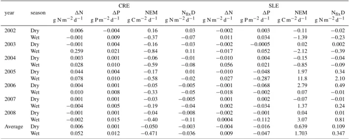
Table 4.Rates of internal dissolved CNP turnover resulting from seasonal DIN and DIP budgets of CRE and SLE from 2002 to 2008. Net internal production or consumption of DIN and DIP were derived through a budgeting process that incorporates water, salt, and input concentrations (1N, g N m−2d−1;1P, g P m−2d−1; Swaney et al., 2011). The DIP rate was converted to net ecosystem metabolism (NEM; g C m−2d−1). Average values were calculated across all dry and all wet seasons, respectively.
CRE SLE
year season 1N 1P NEM NfixD 1N 1P NEM NfixD
g N m−2d−1 g P m−2d−1 g C m−2d−1 g N m−2d−1 g N m−2d−1 g P m−2d−1 g C m−2d−1 g N m−2d−1
2002 Dry 0.006 −0.004 0.16 0.03 −0.002 0.003 −0.11 −0.02
Wet −0.001 0.009 −0.37 −0.07 0.011 0.034 −1.39 −0.23
2003 Dry −0.001 0.004 −0.16 −0.03 −0.002 −0.0005 0.02 0.002
Wet 0.259 0.021 −0.84 0.11 −0.017 0.052 −2.12 −0.39
2004 Dry 0.003 0.001 −0.06 −0.01 −0.010 0.004 −0.15 −0.04
Wet 0.028 0.010 −0.59 −0.08 0.056 0.021 −0.85 −0.09
2005 Dry 0.044 0.004 −0.17 0.01 −0.010 −0.048 1.97 0.34
Wet 0.078 0.010 −0.58 −0.02 0.027 −0.287 11.8 2.10
2006 Dry 0.004 0.001 −0.05 −0.005 −0.001 −0.068 2.79 0.49
Wet 0.010 0.008 −0.33 −0.05 −0.018 −0.002 0.07 −0.01
2007 Dry 0.001 0.001 −0.03 −0.005 0.001 0.002 −0.07 −0.01
Wet −0.004 0.005 −0.19 −0.04 0.002 −0.034 1.37 0.24
2008 Dry −0.001 0.001 −0.04 −0.008 −0.002 −0.001 0.04 0.01
Wet −0.002 0.015 −0.40 −0.11 0.0004 −0.112 3.07 0.81
Average Dry 0.006 0.001 −0.050 −0.003 −0.004 −0.016 0.639 0.109
Wet 0.052 0.012 −0.471 −0.036 0.009 −0.047 1.703 0.347
majority of the 2002–2008 budgets averaging 0.006 and 0.052 g N m−2d−1for the dry and wet seasons, respectively
(Table 4). Internal DIN production did not dramatically in-crease with the loading of external DIN to the CRE despite a maximum input rate of 0.25 g N m−2d−1in the wet season
of 2003 (Fig. 8a). There was no apparent net DIN production or consumption (∼0.0 g N m−2d−1)by the CRE when T
f ≥10 d (Fig. 9a). Similar to1DIN, internal1DIP was pos-itive averaging 0.001 and 0.012 g P m−2d−1suggesting that
the CRE was heterotrophic (−0.05 to −0.47 g C m−2d−1)
across all seasonal budgets (Table 4, Fig. 7c). There was no discernible relationship between1DIP and DIP loading or flushing time (Figs. 8b, 9b). NEM of the CRE signified a balance between internal production and consumption of pri-mary production over all seasonal budgets. Moreover, aver-age seasonal NfixD was negative in both the dry (−0.003 g
N m−2d−1)and wet (−0.036 g N m−2d−1)seasons
indicat-ing net denitrification with an order of magnitude more oc-curring in the wet season (Table 4). NfixDdid not fluctuate
with NEM in the CRE (Fig. 10a).
3.2 St. Lucie Estuary
Rainfall directly to the surface of the SLE ranged from 0.05 to 0.9×10⁶m3d−1across all seasonal budgets (Fig. 3a).
Ex-cept for the extreme value of 0.9×10⁶m3d−1in the wet
sea-son of 2004, total seasea-sonal rainfall was<0.1×10⁶m3d−1.
Freshwater discharge to the SLE was variable with maximum values of ∼10×106m3d−1 in the wet seasons of 2003–
2005 followed by low inflow for both dry and wet seasons beginning in 2006 (Fig. 3b). Surface water inflow was very low from 2007 to 2008. Basin inflow was proportional to sur-face discharge across all seasons (Fig. 3c).
Salinity in the SLE was inverse to freshwater discharge ranging from 6 to 20 in both wet and dry seasons of 2002– 2004 after which values decreased to<2.0 in the wet season of 2005 (Fig. 4a). The salinity of the SLE decreased from 27.0 to<2.0 with increased freshwater inflow across all wa-ter budgets from 2002 to 2008 (Fig. 5a). Average salinity in-creased to 27.0 in the dry season of 2007 when discharge was least andTf=40 days (Fig. 6a). Estuary-wide, average
DIN concentrations exhibited inter-annual fluctuations simi-lar to patterns of inflow from 2002 to 2008 (Fig. 4b). DINe
ranged 0.09–0.20 g m−3 from 2002 to 2005 before
increas-ing to 0.35 g m−3 in wet season of 2004. Seasonally
aver-aged DIN concentrations decreased in both dry and wet sea-sons from 2006 to 2008. Over all seasonal budgets, the con-centration of DIN in the SLE increased linearly from 0.0 to 0.38 g m−3as external loading approached 0.20 g N m−2d−1
(r2=0.85; Fig. 5b). The relationship between flushing time and DIN suggested that concentrations in the SLE declined hyperbolically reaching a minimum of 0.1 g m−3 when T
f >10 d (Fig. 6b). Wet season DIP concentrations were gen-erally 2.5 times greater than in the dry seasons of 2002–2008 (Fig. 4c, Table 4). DIPe concentration reached an apparent
saturation at 0.20 g m−3 with increased external DIP
load-ing (DIPQ)ranging up to 0.4 g N m−2d−1(Fig. 5c). The
hy-perbolic relationship for DIPe was inverted whenTf served
as the independent variable with concentrations declining as flushing time was>10 d (Fig. 6c).
Table 5.Comparisons among attributes of CRE and SLE. Rate values were averaged across all DIP and DIN budgets derived for each estuary (2002–2008). Shown are estuary surface area, flushing time (Tf), freshwater discharge (Q), daily DIP and DIN loading (DIPQ
and DINQ), internal production (+) or consumption (−) of DIP and DIN (1DIP and1DIN), net ecosystem metabolism (NEM) , and the
relative difference between nitrogen fixation and denitrification (NfixD>0.0=net N2fixation; NfixD<0.0=net denitrification). The final row provides the trophic status in terms of production vs. respiration (+NEM=p > r=autotrophic;−NEM=p < r=heterotrophic). The final column provides the ratio of values between the estuaries (CRE : SLE) in terms of surface area,Tf, Q, and DIPQand DINQ.
Attribute Unit CRE SLE CRE : SLE
Surface Area km2 56 22 2.5
Tf d 18.4 11.4 1.6
Q 106m3d−1 6.3 3.1 2.0
DIPQ g P m−2d−1 0.003 0.005 0.6
DINQ g N m−2d−1 0.005 0.007 0.7
1DIP g P m−2d−1 0.014 −0.031
1DIN g N m−2d−1 0.055 0.002
NEM g C m−2d−1 −0.544 1.171
NfixD g N m−2d−1 −0.043 0.228
Trophic Status pvs.r heterotrophic autotrophic
Table 6.Summary of average DIP and DIN loadings (DIPQ and DINQ) and system DIP (1DIP) and DIN (1DIN) production (+) or consumption (−) from several studies using the LOICZ methods. Similar units were derived among the studies for loadings (moles m−2yr−1) and production/consumption (mmol m−2yr−1). Studies with daily rates were multiplied by 182.5 days to calculate seasonal values that were summed to derive annual estimates. Studies reporting a single daily rate were multiplied by 365 days to derive annual estimates.
DIPQ 1DIP DINQ 1DIN
Reference Estuary Size (km2) T
f(days) mol m−2yr−1 mmol m−2yr−1 mol m−2yr−1 mmol m−2yr−1
Que et al., 2003 Lake Illawarra, Australiaa 35
LIA, 1995 1.37 26.5
Miller, 1998 56 7.43 −119.9
Qu, 2001 33 12.43 −85.8
Hung and Huang, 2005 Tsengwen Estuary, Taiwan 2,3,4b 150, 4.5, 1b −83.0 −4484.6
Gazeau et al., 2005 Randers Fjord, Denmark 23 13 65.7
Boonphakdee and Fujiwara, 2008 Bangakong Estuary, Thailand ∼23 15.2 109.5 930.8 Giordani et al,. 2008 LOICZ and Italian lagoonsc
LOICZ1(n=94) <2500 0.31 146.5 5.3 2423.0
LOICZ2(n=61) 0.11 35.3 2.4 −813.0
LaguNet (n=17) 2 d to 3 yrc 0.04 −13.7 1.2 −761.0
Noriega and Araujo, 2011 Barra da Jangandas Estuary, Brazil 13 8–16 0.11 2190.5 0.03 −1292.8 This Study
CRE 57 18.4 0.08 159.6 0.41 1429.9
SLE 22 11.3 0.65 −367.2 0.97 63.0
aThree different studies applied the LOICZ budgeting methods to the Lake Illawarra estuary in Australia.bThe Tsengwen Estuary includes dry, wet, and flood seasons with different values for estuary size and flushing time.c
LOICZ metrics for a network of Italian lagoons (LaguNet) were compared to those derived for a group of estuaries that were<2500 km2in size (LOICZ
1;n=94) and a sub-set of smaller estuaries (LOICZ2;n=61).Tfestimates
varied greatly among the 17 Italian lagoons.
external DINQ up to a maximum loading rate of 0.18 g
N m−2d−1in the wet season of 2004 (Fig. 8a). Net estuarine
DIN production/consumption hovered near 0.0 g N m−2d−1
whenTf≥10 d (Fig. 9a).
1DIP within the SLE was more variable and revealing than1DIN. The SLE generally produced DIP (1DIP>0.0) in the wet seasons of 2002–2004 (Fig. 7b; Table 4). How-ever, DIP was consumed (1DIP<0.0) at rates of−0.05 to
−0.30 g P m−2d−1in 2005 and the dry season of 2006.
In-ternal DIP consumption became more negative as DIPQ
in-creased to 0.4 g P m−2d−1(Fig. 8b). Similar to DIN
dynam-ics, 1DIP was near zero when Tf ≥10 d (Fig. 9b). NEM
was inverse to internal DIP consumption with maximum
val-ues of 1.0–12.0 g C m−2d−1(Fig. 7c) that increased linearly
with the external DIP load (Fig. 8c). Thus, both1DIP and NEM approached 0.0 whenTf≥10 d (Fig. 9b, c). The
av-erage relative difference between N2 fixation and
denitrifi-cation (NfixD) was positive in both dry (0.109 g N m−2d−1)
and wet seasons (0.347 g N m−2d−1)in the SLE (Table 4).
The proportion of N2 fixation (NfixD>0.0) increased
lin-early with NEM, which increased with external DIP loading (Fig. 10a). Closer inspection revealed that SLE ecosystem metabolism may be sensitive to the DIN : DIP loading ratio as NEM (g C m−2d−1)and relative N
2fixation (g N m−2d−1)
Fig. 3.Comparative seasonal time series of water budget compo-nents for CRE and SLE. CRE (filled) and SLE (open) bars are paired seasonally with the first pair of each year representing the dry sea-son. All values are in 106m3d−1.(A)Rainfall;(B)discharge;(C) basin inflow=tributaries+ground water.
2005 had the lowest DIN : DIP loading ratio (∼1.0), the most NEM (∼12 g C m−2d−1), and the greatest relative N fixation
(∼2.2 g N m−2d−1).
4 Discussion
The Caloosahatchee and St. Lucie estuaries on opposite sides of Florida are small, sub-tropical water bodies with highly modified watersheds (Barnes, 2005; Sime, 2005). While nat-ural variations in freshwater inflow and associated salinity changes are part of estuarine dynamics, anthropogenic mod-ification of water delivery to afford flood protection and public safety can create unstable salinity distributions that adversely affect estuarine biota. The direct physical conse-quences of high flow events in the wet season can lead to low salinity throughout both of these estuaries. Rapid de-creases in salinity can make it difficult for benthic organ-isms such as oysters and seagrass to survive (Buzzellli et al., 2012, 2013a). Conversely, periods with low freshwa-ter input indicative of the dry season permits upstream
in-02 03 04 05 06 07 08 09 Se
0 5 10 15 20 25 30
CRE SLE
02 03 04 05 06 07 08 09
DI
N
(g
m
-3)
0.0 0.1 0.2 0.3 0.4
CRE SLE
02 03 04 05 06 07 08 09
DI
P
(g
m
-3)
0.00 0.05 0.10 0.15 0.20 0.25
CRE SLE
(A)
(B)
(C)
Fig. 4.Comparative seasonal time series of water budget compo-nents for CRE and SLE. CRE (filled) and SLE (open) bars are paired seasonally with the first pair of each year representing the dry sea-son.(A)Salinity;(B)DIN (g m−3);(C)DIP (g m−3).
trusion of saltier water that endangers estuarine organisms with freshwater-dependent life cycles (Adams et al., 2009; Tolley et al., 2010; Simpfendorfer et al., 2011). Although both coastal water bodies possess similar watershed patterns of agriculture and urbanization and ranges in flushing time, these two estuaries have very different biogeochemical at-tributes (Table 5).
This study demonstrated that the CRE responded to ex-ternal DIN loading by producing inex-ternal DIN at an aver-age rate of 1429 mmol m−2yr−1(Table 6). A similar result
was reported for the 23 km2, sub-tropical Bangakong Estu-ary in Thailand (930.8 mmol m−2yr−1), which has a flushing
VQ (106 m3 d-1)
0 5 10 15 20 25
Se 0 5 10 15 20 25 30
DINQ (gN m-2 d-1)
0.00 0.05 0.10 0.15 0.20
DI Ne (g m -3) 0.0 0.1 0.2 0.3 0.4
DIPQ (gP m-2 d-1)
0.0 0.1 0.2 0.3 0.4 0.5
DI Pe (g m -3) 0.00 0.05 0.10 0.15 0.20 0.25 (A) (B) (C)
r2= 0.85
DINe= 1.4*DINQ+ 0.08
CRE SLE CRE SLE )] . ( ( * . [ . Q Q e DIP DIP DIP 02 0 15 0 06 0
r2= 0.34
CRE SLE
Fig. 5.Scatter plots from seasonal DIN and DIP budgets for CRE
and SLE from 2002 to 2008.(A)Freshwater discharge (VQ)vs.
estuary salinity;(B)external DIN load (g N m−2d−1)vs. estuary DIN concentration (g m−3);(C)external DIP load (g P m−2d−1) vs. estuary DIP concentration (g m−3). Regression lines,r2values, and equations provided for the SLE points only.
Compared to the CRE, the response of the SLE to DIN loading was less clear with N2fixation in excess of
denitri-fication for all seasonal budgets. Empirical measurements of denitrification from both estuaries reinforced the notion that denitrification is an important sink for nitrogen in the CRE but not the SLE (Table 5; Howes et al., 2008, b). It is sus-pected that biogeochemical feedbacks including coupling of nitrification–denitrification at the sediment–water interface could account for the observed differences between the CRE and SLE (Kemp et al., 2005). The water column is more iso-lated from the benthos in the SLE due to the presence of muck-like sediments and considerably reduced light penetra-tion across the estuary (Sime, 2005; Buzzelli et al., 2013b). Since LOICZ results are dependent upon stoichiometric as-sumptions and DIP dynamics, it is possible that DIN budgets are confounded in benthic-dominated estuaries with low DIN concentrations and significant denitrification (Swaney et al., 2011). This could be the case for the CRE.
Tf (days)
0 10 20 30 40 50 60 70
Se 0 5 10 15 20 25 30 Tf (days)
0 20 40 60
DI Ne (g m -3) 0.0 0.1 0.2 0.3 0.4 Tf (days)
0 20 40 60
DI Pe (g m -3) 0.00 0.05 0.10 0.15 0.20 0.25 (A) (B) (C) CRE SLE CRE SLE CRE SLE ) . ( . f e T DIN 6 4 8 1
r2= 0.60
) . ( . f e T DIP 5 10 2 2
r2= 0.33
Fig. 6.Scatter plots from seasonal DIN and DIP budgets for CRE and SLE from 2002 to 2008. Estimated flushing time (Tf; days) pro-vided the independent variable vs.(A)salinity; (B)estuary DIN concentration (g m−3);(C)estuary DIP concentration (g m−3). Re-gression lines,r2values, and equations provided for the SLE points only.
The budgets revealed that the internal production of C, N, and P was more influenced by external loading to the SLE than the CRE. While the CRE is 2.5 times larger and receives twice the freshwater inflow, spatially normal-ized DIP and DIN loadings are only 60–70 % of those to the SLE (Table 5). Water column DIP concentrations, DIP consumption, and system autotrophy increased with exter-nal DIP loading to the SLE. A similar positive relation-ship between DIP loading and net primary production has been reported for an estuary in Taiwan and several eutro-phied Italian lagoons (Table 6; Hung and Huang, 2005; Gior-dani et al., 2008). In contrast, annual estimates of 1DIP were positive in estuaries such as Randers Fjord, Denmark (65.7 mmol m−2yr−1; Gazeau et al., 2005); Bangakong
Es-tuary, Thailand (109.5 mmol m−2yr−1; Boonphakdee and
Fujiwara, 2008); and the CRE (159.6 mmol m−2yr−1; this
Fig. 7. Comparative seasonal time series of internal CNP source/sink processing for CRE and SLE. CRE (filled) and SLE (open) bars are paired seasonally with the first pair of each year representing the dry season.(A)1DIN (g N m−2d−1);(B)1DIP (g P m−2d−1);(C)NEM (g C m−2d−1).
Florida estuaries (Koch et al., 2011), there is additional po-tential for eutrophication of the SLE through combined water column and benthic regeneration of DIP that fuels primary production (Buzzelli et al., 2013b).
The magnitude of freshwater, DIN, and DIP inputs rel-ative to the flushing time provide the setting for interest-ing biogeochemical dynamics in the SLE (Dettman 2001; Sheldon and Alber, 2006). In the absence of freshwater in-flow, the flushing time of the SLE is approximately 20 d solely through tidal exchange (Y. Wan and D. Sun, unpub-lished data). Nutrient budget results suggested that both the concentrations and internal utilization of DIP and DIN sta-bilized with flushing times greater than 10 d. Longer water residence times allow for increased grazing and sedimenta-tion to respond to primary producsedimenta-tion and balance system metabolism (Buzzelli et al., 2007; Lucas et al., 2009; Phlips et al., 2011; Swaney et al., 2011). In fact, it appears that the negative relationship between flushing time and NEM ob-served in this study is a common attribute of many estuar-ies (Fig. 11). IfTfin the SLE is <10 d as it is much of the
time (Ji et al., 2007), then the inputs of freshwater and
nu-DIPQ (gP m-2 d-1)
0.0 0.1 0.2 0.3 0.4 0.5 -4
0 4 8 12 16
DIPQ (gP m-2 d-1)
0.0 0.1 0.2 0.3 0.4 0.5 -0.4
-0.3 -0.2 -0.1 0.0 0.1
DINQ (gN m-2 d-1)
0.00 0.05 0.10 0.15 0.20 -0.05
0.00 0.05 0.10 0.15 0.20 0.25 0.30
(A)
(B)
(C)
∆ DI
N (
gN
m
-2 d -1)
∆ D
IP
(
gP
m
-2
d
-1)
NEM
(
gC
m
-2 d -1)
CRE SLE
CRE SLE
CRE SLE
r2= 0.53
∆ DIN = 0.27*DINQ+ 0.01
r2= 0.8
∆ DIP = -0.7*DIPQ+ 0.02
r2= 0.8
NEM = 28.3*DIPQ–0.86
Fig. 8.Scatter plots from seasonal DIN and DIP budgets for CRE
and SLE from 2002 to 2008.(A)1DIN (g N m−2d−1);(B)1
DIP (g P m−2d−1);(C)NEM (g C m−2d−1). External DIN load (g N m−2d−1)or DIP load (g P m−2d−1)provided the independent variable. Regression lines,r2values, and equations provided for the SLE points only.
trients result in rapid DIP consumption, a spike in autotro-phy, increased N2fixation, and the potential for DIN export
to the coastal ocean. For example, rates of estuarine DIP consumption (−3.0 g P m−2d−1), NEM (12 g C m−2d−1),
and NfixD (2.3 g N m−2d−1)were all maximized in the wet
season of 2005. In the case of extreme freshwater inflows and rapid flushing (Tf <1 d), both allochthonous and
au-tochthonous materials are transported from the estuary to the coastal ocean (Doering et al., 2006; Murrell et al., 2007; Phlips et al., 2011). Reliable estimates of freshwater inflow and nutrients along with knowledge of flushing time offer a platform to quantify and link external loading to internal ecosystem metabolism (Fig. 11; Dettmann, 2001; Sheldon and Alber, 2006; Swaney et al., 2011).
Tf (days)
0 10 20 30 40 50 60 70 -4 0 4 8 12 16 Tf (days)
0 10 20 30 40 50 60 70 -0.4 -0.3 -0.2 -0.1 0.0 0.1 Tf (days)
0 10 20 30 40 50 60 70 -0.05 0.00 0.05 0.10 0.15 0.20 0.25 0.30 (A) (B) (C) ∆ DI N ( gN m -2 d -1) ∆ DI P ( gP m -2 d -1) NEM ( gC m -2 d -1) CRE SLE CRE SLE CRE SLE
Fig. 9.Scatter plots from seasonal DIN and DIP budgets for CRE and SLE from 2002 to 2008. Estimated flushing time (Tf; days) pro-vided the independent variable vs.(A)1DIN (g N m−2d−1);(B)
1DIP (g P m−2d−1);(C)NEM (g C m−2d−1).
N loading could decrease primary production in the SLE (Phlips et al., 2011). This result is reasonable given that N has been emphasized as the dominant limiting nutrient in es-tuaries (Howarth and Marino, 2006). However, the extrapo-lation of knowledge gained from fine-scale experiments to the seasonal estuary scale may not be appropriate because of feedbacks related to internal biogeochemical cycling (Kemp et al., 2005; Wulff et al., 2011). This may be particularly true for N and P recycling within the SLE where there is surplus DIN produced under increased DIP loading. While increased freshwater inflow could provide the DIP required for N2
fix-ation, it is possible that benthic nitrogen fixation may be in-hibited by lack of light penetration in the SLE (Howarth and Marino, 2006; Buzzelli et al., 2013b). Despite the result that N2fixation exceeded denitrification in the SLE, it is
possi-ble that N2fixation may be negligible since the
phytoplank-ton community is composed of diatoms and dinoflagellates (Millie et al., 2004; Phlips et al., 2011). Smith (1990)
hy-Molar NPQ
0 1 2 3 4 5 6 7
-4 -2 0 2 4 6 8 10 12 14 (C) NE M ( gC m -2 d -1)
r2= 0.4
NEM = -1.3*NPQ+ 4.7
Molar NPQ
0 1 2 3 4 5 6 7
-1.0 -0.5 0.0 0.5 1.0 1.5 2.0 2.5 Wet05 Wet08 Dry06 Wet07 Dry08 Dry05 Dry07Wet04 Dry03 Wet02
Dry02Wet06 Dry04
Wet03 (B) Nfi x D (gN m -2 d -1)
r2= 0.4
NfixD= -0.25*NPQ+ 0.9
-4 -2 0 2 4 6 8 10 12 14 -1.0 -0.5 0.0 0.5 1.0 1.5 2.0 2.5
NEM (gC m-2 d-1) Nfi x D (gN m -2 d -1) CRE SLE
r2= 0.98
NfixD= 0.18*NEM+ 0.02
(A)
Fig. 10.Scatter plots from seasonal DIN and DIP budgets for CRE and SLE from 2002 to 2008.(A)Both the CRE (filled circles) and the SLE (open squares) presented with net ecosystem metabolism (NEM) vs. the difference between N2fixation and denitrification (NfixD). Regression lines,r2 values, and equations provided for the SLE points only.(B)Scatter plots of seasonal values from the SLE from 2002 to 2008. Relationship between the DIN : DIP ratio of loading (independent) and NfixD (dependent).(C)Relationship between the DIN : DIP ratio of loading as the independent variable and NEM as the dependent variable.
pothesized that when DIN supply is great, non-heterocystous phytoplankton can proliferate if provided with adequate P supply. This appears to be the case as the SLE experienced a huge bloom of the toxic, non-heterocystous cyanobacterium
Microcystis aeruginosawith the extreme inputs of freshwater
log Tf (days)
0.0 0.5 1.0 1.5 2.0
log
NE
M
(
m
m
olC m
-2 d -1)
0.0 0.5 1.0 1.5 2.0 2.5
r2= 0.72
log(NEM) = -0.88* log(Tf) + 2.1
N = 19
CRE SLE
(B) (A)
Fig. 11.Integrated results demonstrating the relationship between flushing time (Tf; days) and NEM (mmol C m−2d−1).(A)Plot of estuaries from the LOICZ database with negative NEM, adopted with permission from Swaney et al. (2011).(B)Similar results from the CRE and SLE confined to seasonal budgets with negative NEM (NCRE=13; NSLE=6). Values resulted from log transformation of the absolute values of NEM in each of the 19 cases. Provided are the linear regression information and 95 % confidence intervals (dashed lines).
The recognition that sub-tropical estuaries have the poten-tial to respond to both N and P inputs is an important step to establish nutrient load limits (Smith et al., 2006; Howarth and Marino, 2006; Wulff et al., 2011). However, merely setting criteria for either total or dissolved nutrient loading based on their correlation to water column concentrations fails to appreciate the complexity and uncertainty of estuarine bio-geochemical cycling (Dodds, 2003). In both the discharge and the receiving basin, the DIN : DIP ratios are often very different than the TN : TP ratios due to the differential com-position and reactivity of dissolved organic N and P (DON and DOP; Smith et al., 2005). The assessment of particulate and dissolved organic fractions of the TN and TP pools re-quires a modification of the existing LOICZ protocol (Hung and Huang, 2005).
Freshwater inflow to the SLE has a comparatively high TN : TP ratio (∼14:1), but a much reduced DIN : DIP ra-tio (∼3.0; Doering 1996; SFWMD 2012a). While most of the TP is available as DIP (DIP : TP=0.7), most of the TN is in the form of DON with DIN comprising only 30 % of TN. It is possible that autochthonous DOP production and contri-bution to NEM could confound LOICZ results in some estu-aries (Gazeau et al., 2005). DON is a potentially important component in CNP cycling in CRE, which possesses com-paratively low concentrations of water column N (Hung and Huang, 2005; Eyre et al., 2011). Like many estuaries, there is limited understanding about the effects of DOP and DON cycling on primary production and system metabolism in the SLE and CRE (Smith and Hollibaugh, 2006; Loh, 2008). Fu-ture studies should examine the partitioning and reactivity of TP and TN external loading and internal concentrations in-cluding dissolved and particulate organic and inorganic frac-tions. Knowledge of the role and reactivity of TN and TP constituents would support the contention that the regulation of both nutrients should be considered (Smith, 2006; Paerl, 2009; Conley et al., 2009).
LOICZ was designed to estimate carbon metabolism for estuaries around the world where salinity and inorganic nu-trient concentrations, and not biogeochemical rate processes, provided a bulk of the available data (Swaney et al., 2011). The approach assumes that estuaries can be represented as well-mixed, homogeneous boxes. This assumption cre-ates the potential for errors if an estuary possesses spatial and/or vertical variability in conservative (salinity) and non-conservative (CNP) properties (Webster et al., 2000). While the CRE and the SLE are often well-mixed over depth, there can be horizontal gradients between the headwaters and the oceanic boundary during some inflow conditions (Buzzelli et al., 2013b). A modification that could improve the relia-bility of the LOICZ approach would be to split each estuary into segments based upon predominant salinity and nutrient gradients in the dry and wet seasons. To further refine the approach, in situ rates of dissolved CNP exchanges across the sediment–water interface for different years could be in-troduced to improve system-level calculations and estimates (Buzzelli et al., 2013b).
Smaller estuaries such as the CRE and SLE that are sub-jected to high material loading and fast flushing are very im-portant components in biogeochemical cycling at the local, regional, and global scales (Smith et al., 2005). The LOICZ approach to estuarine nutrient budgets offers a highly trans-ferrable method to link watershed inputs to biogeochemical responses for a variety of coastal embayments (Swaney et al., 2011). While the LOICZ approach has been applied to hun-dreds of coastal water bodies, its value to coastal manage-ment is dependent upon the quality of input data, the reliabil-ity of the steady-state and stoichiometric assumptions, and the connectivity between the watersheds and the estuaries (Smith et al., 2005; Swaney et al., 2011). This study provided an improved understanding of the relationships among sea-sonal variations in watershed N and P loading, hydrodynamic flushing time, nutrient cycling, and ecosystem metabolism for sub-tropical estuaries with heavily modified watersheds (Millie et al., 2004; Phlips et al., 2011; Eyre et al., 2011).
Acknowledgements. We would like to thank Kathy Haunert,
Zhiquiang Chen, Detong Sun, Lucia Baldwin, Nenad Irichanin, and Daniel Crean for help in data acquisition. Yao Yan helped provided geographic expertise for map Figs. 1 and 2. A special acknowledgement goes to Dennis Swaney for valuable insight into the LOICZ approach and interpretation of results. We acknowledge the editorial efforts of P. Gorman, S. Gray, and R. T. James at the South Florida Water Management District and four anonymous reviewers.
Edited by: B. A. Bergamaschi
References
Adams, A. J., Wolfe, R. K., and Layman, C. A.: Preliminary exam-ination of how human-driven freshwater flow alteration affects trophic ecology of juvenile snook (Centropomus undecimalis) in estuarine creeks, Estuar. Coast., 32, 819–828, 2009.
Antonini, G. A., Fann, D. A., and Roat, P.: A Historical Geogra-phy of Southwest Florida Waterways. Volume II; Placida Harbor to Marco Island, National Sea Grant College Program, College Park, MD, 1–16, 2002.
Barnes, T.: Caloosahatchee Estuary Conceptual Ecological Model, Wetlands, 25, 884–897, 2005.
Boonphakdee, T. and Fujiwara, T.: Temporal variability of nutrient budgets in a tropical river estuary: The Bangpakong River Estu-ary, Thailand, Environment Asia, 1, 7–21, 2008.
Brock, D. A.: Nitrogen budget for low and high freshwater inflows, Nueces Estuary, Texas, Estuaries, 24, 509–521, 2001.
Buranapratheprat, A., Yanagi, T., Boophakdee, T., and Sawang-wong, P.: Seasonal variations in inorganic nutrient budgets of the Bangpakong Estuary, Thailand, J. Oceanogr., 58, 557–564, 2002. Buzzelli, C., Holland, A. F., Sanger, D. S., and Conrads, P. C.: Hy-drographic characterization of two tidal creeks with implications for watershed land use, flushing times, and benthic production, Estuar. Coast., 30, 321–330, 2007.
Buzzelli, C., Robbins, R., Doering, P., Chen, Z., Sun, D., Wan, Y., Welch, B., and Schwarzchild, A.: Monitoring and modeling of
Syringodium filiforme (Manatee Grass) in the southern Indian River Lagoon, Estuar. Coast., 35, 1401–1415, 2012.
Buzzelli, C., Parker, M., Geiger, S., Wan, Y., Doering, P., and Haunert, D.: Predicting system-scale impacts of oyster clearance on phytoplankton production in a small sub-tropical estuary, En-viron. Model. Assess., 18, 185–198, 2013a.
Buzzelli, C., Chen, Z., Coley, T., Doering, P., Samimy, R., Schlezinger, D., and Howes, B.: Dry season sediment-water ex-changes of nutrients and oxygen in two Florida estuaries: Pat-terns, comparisons, and internal loading, Florida Scientist, 76, 54–79, 2013b.
Chamberlain, R. H. and Doering, P. H.: Freshwater inflow to the Caloosahatchee Estuary and the resource-based method for eval-uation, in: Proceedings of the Charlotte Harbor Public Confer-ence and Technical Symposium, edited by: Treat, S. F., South Florida Water Management District, West Palm Beach, FL, 81– 90, 1998.
Childers , D. L., Boyer, J. N., Davis, S. E., Madden, C. J., Rudnick, D. T., and Sklar, F.: Relating precipitation and water management to nutrient concentrations in the oligotrophic “upside-down” es-tuaries of the Florida Everglades, Limnol. Oceanogr., 51, 602– 616, 2006.
Cloern, J. E.: Our evolving conceptual model of the coastal eutroph-ication problem, Mar. Ecol. Prog. Ser., 210, 223–253, 2001 Conley, D. J., Paerl, H. W., Howarth, R. W., Boesch, D. F.,
Seitzinger, S. P., Havens, K. E., Lancelot, C., and Likens, G. E.: Controlling eutrophication: Nitrogen and phosphorus, Science, 323, 1014–1015, 2009.
Dennison, W. C.: Environmental problem solving in coastal ecosys-tems: A paradigm shift to sustainability, Estuar. Coast. Shelf Sci., 77, 185–196, 2008.
Dettmann, E. H.: Effect of water residence time on annual export and denitrification of nitrogen in estuaries: A model analysis, Es-tuaries, 24, 481–490, 2001.
Dodds, W. K.: Misuse of inorganic N and soluble reactive P con-centrations to indicate nutrient status of surface waters, J. North Amer. Benthol. Soc., 22, 171–181, 2003.
Doering, P. H.: Temporal variability of water quality in the St. Lucie Estuary, South Florida, Water Res. Bull., 32, 1293–1306, 1996. Doering, P. H., Chamberlain, R., and Haunert, K. M.: Chlorophyll
a and its use as an indicator of eutrophication in the Caloosa-hatchee Estuary, Florida, Florida Scientist, 69, 51–72, 2006. Eyre, B., Ferguson, A. J. P., Webb, A., Maher, D., and Oakes, J. M.:
Denitrification, N-fixation, and nitrogen and phosphorus fluxes in different benthic habitats and their contribution to the nitro-gen and phosphorus budgets of a shallow oligotrophic subtrop-ical coastal system (southern Moreton Bay, Australia), Biogeo-chemistry, 102, 111–133, 2011.
Flemer, D. A. and Champ, M. A.: What is the future fate of estuar-ies given nutrient over-enrichment, freshwater diversion, and low flows?, Mar. Pollut. Bull., 52, 247–258, 2006.
Gazeau, F., Borges, A.V., Barron, C., Duarte, C.M., Iversen, N., Middleburg, J.J., Delille, B., Pizay, M.-D., Frankingnoulle, M., and Gattuso, J.-P.: Net ecosystem metabolism in micro-tidal estu-ary (Randers Fjord, Denmark): evaluation of methods, Mar. Ecol. Prog. Ser., 301, 23–41, 2005.
ap-plication of the LOICZ biogeochemical model, Estuar. Coast. Shelf Sci., 77, 264–277, 2008.
Gordon, D. C., Boudreau, P. R., Mann, K. H., Ong, J.-E., Silvert, W. L., Smith, S. V., Wattayakorn, G., Wulff, F., and Yanagi, T.: LOICZ Biogeochemical Modeling Guidelines, LOICZ/R&S/95-5, Texel, the Netherlands, 1–96, 1996.
Howarth, R. W. and Marino, R.: Nitrogen as the limiting nutrient for eutrophication in coastal marine ecosystems: evolving views over three decades, Limnol. Oceanogr., 51, 364–376, 2006. Howes, B. H., Schlezinger, D., and Samimy R.: The
Character-ization and Quantification of Benthic Nutrient Fluxes in the Caloosahatchee River and Estuary. Project Summary Report, Coastal Systems Program, School for Marine Science and Tech-nology, University of Massachusetts Dartmouth, 2008a. Howes, B. H., Schlezinger, D., and Samimy R.: The
Characteriza-tion and QuantificaCharacteriza-tion of Benthic Nutrient Fluxes in the St. Lu-cie River and Estuary. Project Summary Report, Coastal Systems Program, School for Marine Science and Technology, University of Massachusetts Dartmouth, 2008b.
Hung, J. J. and Huang, M. H.: Seasonal variations in organic car-bon and nutrient transport through a tropical estuary (Tsengwen) in southeastern Taiwan, Environ. Geochem. Health, 27, 75–95, 2005.
Ji, Z.-G., Hu, G., Shen, J., and Wan, Y.: Three-dimensional model-ing of hydrodynamics processes in the St. Lucie Estuary, Estuar. Coast. Shelf Sci., 73, 188–200, 2007.
Kemp, W. M., Boynton, W. R., Adolf, J. E., Boesch, D. F., Boicourt, W. C., Brush, G., Cornwell, J. C, Fisher, T. R., Glibert, P. M., Hagy, J. D., Harding, L. W., Houde, E. D., Kimmel, D. G., Miller, W. D., Newell, R. I. E., Roman, M. R., Smith, E. M., and Steven-son, J. C.: Eutrophication of Chesapeake Bay: Historical trends and ecological interactions, Mar. Ecol. Prog. Ser., 303, 1–29, 2005.
Koch, G. R., Childers, D. L., Staehr, P. A., Price, R. M., Davis, S. E., and Gaiser, E. E.: Hydrological conditions control P load-ing and aquatic metabolism in an oligotrophic subtropical estu-ary, Estuar. Coast., 35, 335–352, doi:10.1007/s12237-011-9431-5, 2011.
Liu, S. M., Hong, G.-H., Zhang, J., Ye, X. W., and Jiang, X. L.: Nutrient budgets for large Chinese estuaries, Biogeosciences, 6, 2245–2263, doi:10.5194/bg-6-2245-2009, 2009.
Loh, A.: Mixing and Degradation of Riverine Dissolved Organic Nitrogen in the Caloosahatchee Estuary. Final Report to the South Florida Water Management District, 35 pp., 2008. Lucas, L. V., Thompson, J. K., and Brown, L. R.: Why are
di-verse relationships observed between phytoplankton biomass and transport time?, Limnol. Oceanogr., 54, 381–390, 2009. Millie, D. F., Carrick, H. J., Doering, P. H., and Steidinger, K. A.:
Intra-annual variability of water quality and phytoplankton in the North Fork of the St. Lucie River Estuary, Florida (USA): a quan-titative assessment, Estuar. Coast. Shelf Sci., 61, 137–149, 2004. Murrell, M., Hagy, J. D., Lores, E. M., and Greene, R. M.: Phy-toplankton production and nutrient distributions in a subtropical estuary: Importance of freshwater flow, Estuar. Coast., 30, 390– 402, 2007.
Nixon, S. W.: Coastal marine eutrophication: A definition, social causes, and future concerns, Ophelia, 41, 199–219, 1995.
Noriega, C. E. D. and Araujo, M.: Nutrient budgets (C, N, P) and trophic dynamics of a Brazilian tropical estuary: Barra das Jan-gadas, Ann. Braz. Ac. Sci., 83, 441–456, 2011.
Paerl, H. W.: Controlling eutrophication along the freshwater-marine continuum: Dual nutrient (N and P) reductions are es-sential, Estuar. Coast., 32, 593–601, 2009.
Phlips, E. J., Badylak, S., Hart, J., Haunert, D., Lockwood, J., O’Donnell, K., Sun, D., Viveros, P., and Yilmaz, M.: Climatic influences on autochthonous and allochthonous phytoplankton biomass in a subtropical estuary, St. Lucie Estuary, Florida, USA, Estuar. Coast., 35, 292–307, doi:10.1007/s/12237-011-9442-2, 2011.
RECOVER: System Status Report, Restoration Coordination and Verification Program, United States Army Corps of Engineers, Jacksonville, FL, and the South Florida Water Management Dis-trict, West Palm Beach, FL, 2010.
Sackett, J. W.: Survey of the Caloosahatchee River, Florida. Report to the Captain of the United States Engineering Office, St. Au-gustine, Florida, 1888.
SFWMD: St. Lucie River Watershed Protection Plan 2012 Update, 2012 South Florida Environmental Report, Volume 1, Appendix 10-1, available at: www.sfwmd.gov/SFER, 2012a.
SFWMD: Caloosahatchee River Watershed Protection Plan 2012 Update, 2012 South Florida Environmental Report, Volume 1, Appendix 10-2, available at: www.sfwmd.gov/SFER, 2012b. Sheldon, J. E. and Alber, M.: The calculation of estuarine turnover
times using freshwater fraction and tidal prism methods: A criti-cal evaluation, Estuaries and Coasts, 29, 133-146, 2006. Sime, P.: St. Lucie Estuary and Indian River Lagoon Conceptual
Ecological Model, Wetlands, 25, 898–207, 2005.
Simpfendorfer, C. A., Yeiser, B. G., Wiley, T. R., Poulakis, G. R., Stevens, P. W., and Heupel, M. R.: Environmental influences on the spatial ecology of juvenile smalltooth sawfish (Pristis pecti-nata): Results from acoustic monitoring, Plos One, 6, 1–12, 2011. Smith, V. H.: Nitrogen, phosphorus, and nitrogen fixation in lacus-trine and estuarine ecosystems, Limnol. Oceanogr., 35, 1852– 1859, 1990.
Smith, V. H.: Responses of estuarine and coastal marine phy-toplankton to nitrogen and phosphorus enrichment, Limnol. Oceanogr., 51, 377–384, 2006.
Smith, S. V. and Hollibaugh, J. T.: Water, salt, and nutrient ex-changes in San Francisco Bay, Limnol. Oceanogr., 51, 504–517, 2006.
Smith, S. V., Swaney, D. P., Talaue-McManus, L., Bartley, J. D., Sandhei, P. T., McLaughlin, C. J., Dupra, V. C., Crossland, C. J., Buddemeier, R. W., Maxwell, B. A., and Wulff, F.: Humans, hydrology, and the distribution of inorganic nutrient loading to the ocean, Bioscience, 53, 235–245, 2003.
Smith, S. V., Buddmeier, R. W., Wulff, F., Swaney, D. P.: C, N, P fluxes in the coastal zone, edited by Crossland, C. J., Kre-mer, H. H., Lindeboom, H. J., Marshall-Crossland, J. I, and Le Tissier, M. D. A.: Coastal Fluxes in the Anthropocene. The Land-Ocean Interactions in the Coastal Zone Project of the Interna-tional Geosphere-Biosphere Programme, Spring, Berlin, Heidel-berg, Chapter 3, 96–143. 2005.
Swaney, D. P., Smith, S. V., and Wulff, F.: The LOICZ Biogeochem-ical Modeling Protocol and its Application to Estuarine Ecosys-tems in: Estuarine and Coastal Ecosystem Modeling, edited by: Baird, D. and Mehta, A., Academic Press, Amsterdam, Chapter 9, 135–160, 2011.
Talaue-McManus, L., Smith, S. V., and Buddemeier, R. W.: Bio-physical and socio-economic assessments of the coastal zone: the LOICZ approach, Ocean Coast. Manag., 46, 323–333, 2003. Tolley, S. G., Evans, J. T., Burghart, S. E., Winstead, J. T., and
Vo-lety, A. K.: Role of freshwater inflow and salinity on population regulation in the hydrozoan inquiline symbiont Eutima sp., Bull. Mar. Sci., 86, 625–636, 2010.
United States Army: Annual Report of the Chief of Engineers, War Department Document Number 493, Part 1, Government Print-ing Office, WashPrint-ington, DC, 1915.
Webster, I. T., Smith, S. V., and Parslow, J. S.: Implications of spa-tial and temporal variation for biogeochemical budgets of estuar-ies, Estuarestuar-ies, 23, 341–350, 2000.
Wosten, J. H. M., de Willigan, P., Tri, N. H., Lien, T. V., and Smith, S. V.: Nutrient dynamics in mangrove areas of the Red River Es-tuary in Vietnam, Estuar. Coast. Shelf Sci., 57, 65–72, 2003. Wulff, F., Eyre, B., and Johnstone, R.: Nitrogen versus
phospho-rus limitation in a subtropical embayment (Moreton Bay, Aus-tralia): Implications for management, Ecol. Modell., 222, 120– 130, 2011.