A SENSITIVITY STUDY USING TWO DIFFERENT CONVECTION SCHEMES OVER SOUTH
AMERICA
LUCIANO PONZI PEZZI, IRACEMA F. A. CAVALCANTI ANd ANTÔNIO M. MENdONÇA
Centro de Previsão de Tempo e Estudos Climáticos (CPTEC)
Instituto Nacional de Pesquisas Espaciais (INPE)
Cachoeira Paulista, SP, Brasil
[email protected]
Received September 2006 - Accepted October 2007
ABSTRACT
The sensitivity of cumulus convection parameterizations is investigated using the CPTEC/COLA Atmospheric General Circulation Model (AGCM) with T62L28 resolution. This model has been used at CPTEC/INPE since 1995 with the Kuo convective scheme for weather and seasonal climate forecasts. In this study, two sets of integrations are performed using climatological Sea Surface Temperature (SST) of the Southern Hemisphere summer season (december, January and February) as bottom boundary conditions. Five integrations with different initial conditions are applied for each ensemble. The study was divided in two groups, one using the adjusted Relaxed Arakawa-Schubert convection scheme considering modiications in the convection physics (ARAS) and the other one using the Kuo convection scheme (KUO). The atmospheric circulation and precipitation model results are compared with NCEP/NCAR reanalysis data and CMAP precipitation data. The results are analyzed mainly over South America and also for the Southern Hemisphere to verify the model response compared to observed data when different convection scheme is applied. The adjusted scheme for RAS suggested in this study, reduced errors in several areas of South America, when comparing with the previous version. Over most of South America areas KUO gives smaller errors than ARAS. Over tropical Paciic Ocean, Southeastern Brazil and south of northeast Brazil, ARAS scheme shows better results. Keywords: deep convection, Kuo scheme, Arakawa-Schubert scheme, AGCM convection scheme, South America Precipitation, SACZ
RESUMO: ESTUdO dE SENSIBILIdAdE USANdO-SE dOIS ESQUEMAS dIFERENTES dE CONVECÇÃO SOBRE A AMÉRICA dO SUL
1. INTRODUCTION
Atmospheric General Circulation Models (AGCMs) have been used in seasonal climate prediction and climatological experiments in several research centers. In the tropics the large-scale precipitation is dominated by convective activity that depends on the convection scheme adopted in each model. The surface boundary forcing for the atmospheric models is the Sea Surface Temperature (SST) which can have inluence on all parts of the globe. For example, the climate of South America is largely inluenced by the tropical oceanic conditions.
Several studies have shown the effect of El Niño-Southern Oscillation (ENSO) on precipitation over South America. Warm episodes (El Niño) are associated with the occurrence of a weaker rainy season over the Amazon and Northeast Brazil regions, as well as with excessive precipitation over southern Brazil (Kousky et al. 1984, Rao et al. 1986, Ropelewski and Halpert, 1996). Observational studies have shown that the Atlantic SST dipole also inluences South America in the rainy season of Northeast Brazil (Nobre and Shukla, 1996) and the Amazon region (Souza et al., 2000). Numerical model experiments performed by Pezzi and Cavalcanti (2001) showed the inluence of both ENSO and tropical SST Atlantic dipole on precipitation over South America, when they occur simultaneously. The Northeast region (Nordeste) which is situated at 2˚S-18˚S; 45˚W-35˚W, has a high degree of predictability when GCMs are used, as pointed out in several studies such as Graham (1994), Sperber and Palm (1996), Marengo et al. (2003). However, it has been dificult to predict rainfall over the southeastern region of Brazil, correctly. This region is affected by frontal systems during the whole year and by the South Atlantic Convergence Zone (SACZ) in the summer.
Statistical analysis performed by Marengo et al. (2003) showed that the southeastern Brazil region has a large dependence on the initial conditions when the CPTEC/COLA AGCM is applied to simulations or predictions. Results of a climate simulation using CPTEC/COLA AGCM (Cavalcanti et al., 2002) showed the presence of the NW-SE precipitation band in the summer season, over South America/South Atlantic Ocean, representing the SACZ occurrence. However, the model overestimated precipitation in the southern portion of this band, and underestimated precipitation in the tropical sector. This systematic error is partially removed when the precipitation anomalies are taken, but the scheme used in the parameterization of convective precipitation may be responsible for the errors. The southeastern area of Brazil is a densely populated region, which is affected by cases of extreme rainfall associated with the behavior of the SACZ. Thus, improvements in seasonal prediction or better knowledge of the model limitations for the region are required.
Convective precipitation in CPTEC/COLA AGCM is derived from the convection scheme of Kuo (1965). de Witt (1996) and Kirtman and deWitt (1997) showed the possibility of improvements in the COLA AGCM results by changing the convection parameterization scheme. In their studies three convection parameterization schemes were tested, the Kuo (1965) (hereafter KUO) scheme, Betts and Miller (1993) and Relaxed Arakawa-Schubert (Moorthi and Suarez, 1992; Arakawa and Shubert, 1974) (hereafter RAS) scheme. A detailed description of the convection schemes used in the experiments can be found in deWitt (1996). The results from the AGCM model were compared with European Centre for Medium Range Weather Forecast (ECMWF) reanalysis data. The main conclusions were that improvements might be expected by applying the RAS convection scheme.
To evaluate the sensitivity of the COLA AGCM in simulating surface wind stress when the model was submitted to the three different convection schemes, Kirtman and deWitt (1997) forced the Geophysical Fluid dynamics Laboratory (GFDL) ocean model with the three different ields of wind stress obtained from the experiments. Analyzing the output, they compared the results from the ocean model simulation with ocean data assimilation analysis provided by National Center for Environmental Prediction (NCEP). In that study Kirtman and deWitt (1997) showed that some of the errors in the annual cycle and the interannual variability of AGCM wind stress could be attributed to the convective parameterization. Based on their results they found that the RAS convective parameterization gave the best simulation of the annual cycle and interannual variability in the tropical Paciic when the atmospheric model was coupled to the ocean model.
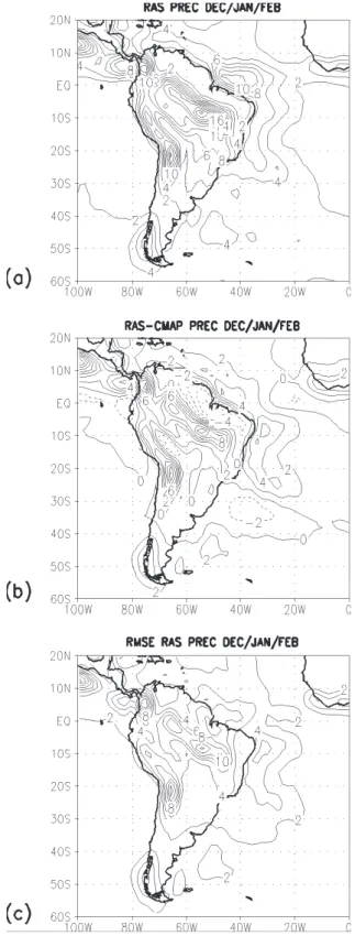
Figure 1 - Results of precipitation using RAS scheme without adjustments, for december, January and February. (a) Precipitation, (b) Precipitation difference (RAS-CMAP), (c) Root mean square error (RMS). Intervals are 2 mm.day-1.
ideas about both KUO and RAS convection schemes as well as the adjustment done in the ARAS scheme are shown in section 2. The experimental design is described in section 3. Precipitation results over South America are discussed in section 4. The extratropical Southern Hemisphere features obtained from the experiments are displayed in section 5. Regional analysis and skill in several areas of South America are discussed in section 6. The inal discussion and conclusions are given in section 7.
2. THE DEEP CONVECTION
PARAMETERIZATIONS AND ADJUSTMENT TO RAS
The AGCM used in this study is the same used by CPTEC for operational climate and weather forecast as well as for research purposes (Pezzi and Cavalcanti, 2001; Cavalcanti et al., 2002; Cavalcanti et al., 1999; Marengo et al., 2003). It is based on previous version of the NCEP global spectral model used for medium range forecast, modiied by COLA (Kinter et al., 1997 and deWitt, 1996) and by CPTEC (Cavalcanti et al. 2002). It is a spectral global model with two options for convection, the KUO and RAS schemes. In this study we conducted two experiments, using the T62L28 resolution (corresponding to approximately 1.88˚), one applying the KUO convection parameterization (Kuo, 1965) and the other one using the RAS convection scheme (Moorthi and Suarez, 1992; Arakawa and Schubert, 1974), however, with modiications in the base and top cloud levels and in the cloud eficiency.
2.1. The KUO scheme
2.2. The RAS scheme
The RAS scheme is described in detail in Moorthi and Suarez (1992): It is a modiication of the original Arakawa and Schubert (1974) scheme. This scheme implemented by COLA differs from the original Arakawa-Schubert version in two aspects: 1) - the normalized lux of mass which is an exponential function of the height is replaced by a linear function of the height; 2) - in the original version the whole cumulus cloud ensemble must be in quasi-equilibrium each time that the cumulus convection routine is called. This will imply that the interaction between the clouds must occur quickly when compared to the changes in the large-scale forcing. The original version assumes that these interactions occur instantaneously and this might result in an overadjustment, in which some cloud types are overstabilized by the effects of other cloud types, i.e., multiple mass-lux distributions can produce the balance for those clouds with positive buoyancy. In RAS scheme, there is no direct interaction between clouds, however, it allows that during the adjustment process each cloud type interact and change the surrounding environment and that the following clouds are affected by this environmental change. In this way, the RAS scheme goes towards equilibrium of a singular cloud, but during the whole integration all clouds will affect each other through the environment. differing from the original version, the RAS scheme, assumes that the cloud-environment interaction occurs in a short and inite time interval so that the large-scale atmosphere is relaxed towards quasi-equilibrium instead of assuming instantaneous interactions as in the original version. The RAS implementation in the CPTEC/COLA AGCM assumes that the sub-cloud layer is composed by the mass weighted averaged of the two lowest model layers. Each time that the cumulus parametrization convection is used, all levels above the sub-cloud layer are checked to access the convection likelihood. Clouds with the same base but with different levels of detrainment (clouds top) are classiied as different kinds of clouds. In the RAS scheme, the cumulus convection occurs for those kinds of clouds where the cloud work function exceeds a critical value which is empirically determined. The cloud work function is the integrated measure of the wet static energy difference between the cloud and the environment. For those kinds of clouds where the cloud work function exceeds a critical value, the mass lux at cloud base needed to restore the cloud work function to its critical value is determined. This mass lux is used to solve the equations on the grid scale, including the convection effects on the temperature and speciic humidity. The re-evaporation of the convective precipitation within the environment is allowed, as suggested by Sud and Molod (1988).
2.3. The adjusted RAS scheme - ARAS
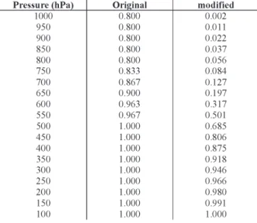
Table 1 - Clouds eficiency as function of pressure at the clouds top
On the other hand, the cloud types are selected according to the detrainment levels, i.e. to all levels above 3 rd, up to the level below the stratosphere. The CPTEC/COLA AGCM model used here has 28 levels in the vertical (L28). It has a non uniform vertical distribution of the thickness layers (more levels near the surface and at the high troposphere) allowing a better representation of the physical processes in the mixed layer and in the region near the tropopause. In the L28 resolution, 7
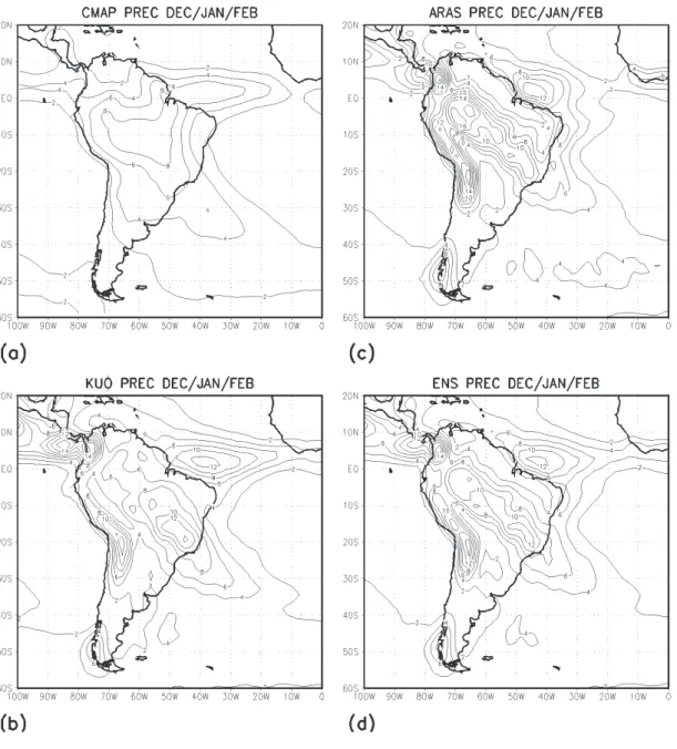
Figure 2 - Contours of climatological precipitation for december,January and February. (a) CMAP , (b) KUO, (c) ARAS and (d) KUO+ARAS. Intervals are 2 mm. day-1.
Precipitation excess represented by the CPTEC/COLA AGCM, using the RAS scheme, might be related to the cloud eficiency on conversion of cloud liquid water into precipitation. The original RAS version gives an eficiency of 80% to clouds with top below 800 hPa. A linear interpolation between 80% and 100% is done for clouds with top between 800 and 500 hPa and 100% is used when the top clouds are above 500 hPa. These eficiencies are large for shallow clouds. New schemes, including the modiications described below have originated the adjusted RAS scheme (ARAS). So the ARAS scheme uses a new proile to cloud eficiency similarly to those suggested by Silva-Dias (1977). This new proile has smaller cloud eficiency than the original version, with major reductions for shallow clouds. Table 1 compares the precipitation eficiency used in RAS and the new ARAS scheme. The second column in this table displays the eficiency values used in the original version while the third column shows the new values suggested and
used in this study. These values are associated with each top cloud pressure which is related to their deepness as indicated in the irst column of Table 1.
3. THE EXPERIMENTAL DESIGN AND ERROR ANALYSIS
For each experiment, ive integrations are performed using the atmospheric conditions of days 13, 15, 16, 17 and 18 of November 1998 as initial data. The model is integrated up to February, using as boundary forcing conditions, the climatological SST monthly ields (averaged over the period from 1950 to 1996) of November to February, obtained from the Reynolds and Smith (1994) SST data set. These data have a horizontal grid resolution of 1˚x 1˚ and the climatological average is used with the purpose of reproducing the mean state of the simulated atmosphere.
Both cumulus convection schemes (KUO and ARAS) are applied for each ensemble of five integrations. The resulting ensemble integrations are analyzed considering the two experiments separately (2 ensembles of 5 integrations each), and also constructing another ensemble with results of the two experiments (average of the two ensembles), called the total ensemble. Observed precipitation is derived from the Climate Prediction Center Merged Analysis Precipitation (CMAP) dataset (Xie and Arkin, 1997), and the NCEP/NCAR reanalysis data (Kalnay et al., 1996) are used to compare wind and geopotential height with model results. The climatological precipitation and other reanalysis variables are calculated for the period of 1979 to 1998. Then, climatological model results are compared to climatological observational data.
To assess the impact of the two different cumulus convection schemes on the climate of CPTEC/COLA AGCM, we followed the analysis presented in \emph{deWitt} (1996) performing the Root Mean Square Error (RMS):
(1)
(2)
M is equal to 15 and refers to the number of months (3) of the 5 integrations. ym represents the ields simulated by the
AGCM and Om the analysis (or observations). Performing the
calculation in this way the error attributed to the dispersion among each individual member is also diagnosed.
4. DJF CLIMATOLOGICAL PRECIPITATION OVER SOUTH AMERICA USING KUO AND ARAS CONVECTION SCHEMES
The precipitation ields (observed and simulated) for the summer season over South America (dJF) are shown in Figure 2 and differences between model and observation are displayed in Figure 3. One of the most typical summer season characteristics over South America is the presence of deep convection in a cloud belt with northwest (NW) to southeast (SE) orientation. This band is associated with the occurrence of the South Atlantic Convergence Zone (SACZ) and contributes considerably to the total amount of precipitation over that region.
Using the KUO scheme, the model overestimates the total precipitation amount in the southern part of the SACZ and underestimates the precipitation over the westernmost region (Figures 2b and 3a). A similar result has been shown also in Cavalcanti et al. (2002). This simulated precipitation pattern by
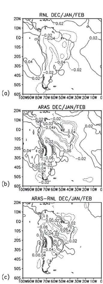
Figure 4 - Moisture convergence (x 103 day-1) at 850 hPa using the
the AGCM apparently is a convection scheme response to the dynamic forcing (moisture convergence in the lowest levels) as observed in Figure 4 and also associated with an excess of wind conluence at low levels (igure not shown). Figures 4b and 4c show that the simulated moisture convergence is larger than that observed in the reanalysis, near 5. 10-3 day-1 against
1.10-3 day-1 respectively, over Southeastern Brazil. It is coincident
with regions where the precipitation is overestimated. This is consistent, since the main triggering convection mechanism in the KUO scheme is the moisture convergence.
Using the ARAS convection scheme, the results are better than the previous RAS implemented in the model, and the errors reduce, but are still large in the precipitation ield over South America. The model enhances precipitation over the tropical region of SACZ, however excessive values occur over western Amazonia and near the northeast Brazil
coast. Underestimated rainfall occurs around the Amazon River mouth and also east of Andes (Figures 2c and 3c). The excessive convection over western Amazon, Nordeste coast and over Andes may be generating an excessive subsidence movement in other areas.The main convection triggering mechanism in the ARAS scheme is the cloud work function which represents an integrated measurement of the difference between the moist static energy (h) and the saturation moist static energy (h*). Figure 5 exhibits the vertical proiles of h and h* for two contrasting points over South America, concerning to the amount of simulated precipitation. Considering the irst point located at 55˚W and 8˚S where the model has an excess of precipitation, we can see that reanalysis proile is favorable to deep convection clouds development because the parcel which is lifted from surface might saturate around 900 hPa level (cloud base) and the cloud top might reach up to 300 hPa level.
Figure 5 - Vertical proiles of the moist static energy (dashed lines) and the saturation moist static energy (solid lines) for two points over South
At this same location the simulated proiles of h e h* (Figure 5b) indicate the presence of a warmer and drier layer between 700 e 1000 hPa with a maximum between 900 and 950 hPa. This will cause an inversion in the environmental thermodynamics properties at the lowest model layers. This effect is not seen in the reanalysis data. Those differences seen in the model simulations will cause an increase of the cloud base heights to approximately 750 hPa. Nevertheless, the vertically integrated differences between h e h* suggest the possibility of deep convection development. The second point is located at 50˚W and 2.5˚S. This location is where the model simulation underestimates the climatological precipitation amount. The reanalysis proiles of h and h* (Figure 5c) are similar to those observed in Figure 5a. Nonetheless, the simulated proiles (Figure 5d) are quite different of those exhibited by the reanalysis, mainly in the layer below 700 hPa. The model layer (between 700 e 1000 hPa) is highly warmer and drier than the observed one. This is a non favorable condition to the cloud development since a parcel of air lifted from the surface will reach the saturation near 700 hPa but the vertically integrated difference between h and h* will be null approximately. As a consequence, the convection is not triggered at this point.
Figure 6 shows the vertical velocity ield (omega) at 500 hPa. It can be seen from Figure 6a, that the central and north regions of South America and the SACZ regions are dominated by ascent vertical movements. The vertical movement pattern agrees with the precipitation ield. For model simulation (Figure 6b), it is noticed an agreement between the ascent movement region with a precipitation excess region and a compensating subsidence region where a precipitation deicit is simulated. These results altogether with Figure 5, suggest that the enhanced ascent simulated by the model over SACZ and central South America regions, is causing a strong subsidence to the northeastern of this convection belt. This subsidence will dry and warm the environment at the lower levels over that region, inhibiting the cloud development and consequently eliminating the production of precipitation along the South America north shore.
Considering the total ensemble (KUO+ARAS), the precipitation is improved on the northwestern Amazon region, and on the southern sector of the SACZ. However, inside the band, the combination of the two schemes still shows overestimated precipitation, but with smoothed values compared to the ARAS scheme (Figures 2d and 2c). The error over the northern coast is reduced and the underestimated values east of Andes are concentrated in a small area (Figure 3b). This latter behavior might be related to the excess of precipitation that remains over the Andes Mountains, a feature mentioned in Cavalcanti et al. (2002). Both the KUO and ARAS convection schemes produce maximum precipitation between 10˚S and 30˚S over the Andes region, with the ARAS scheme producing higher maximum
Hemisphere while the ARAS scheme improved the zonal wind representation in the upper atmosphere of the Northern Hemisphere. Comparing the geopotential height zonal anomalies at 200 hPa from the results of both experiments, it is noticed that the zonal structures are very similar to the observations, but the intensity and position of some of the anomalous zonal centers are better simulated using the ARAS scheme (Figure 10). However, the ARAS scheme gives more intense centers over the southeastern Paciic and southwestern Atlantic. Figure 11 shows the RMS for the 200 hPa geopotential height. For this variable, the ARAS convection scheme shows errors of smaller magnitude than the KUO scheme, mainly around Antarctica (Figures 11a, b, c). With ARAS scheme errors are large over three areas, over the drake Passage (between the southern South America and Antarctic Peninsula), over the southwestern Paciic and over the southern Indian ocean. The errors in both versions relect the deiciency of the model in representing well the intensity and position of jet streams aroundthe Southern Hemisphere. Consistent with the geopotential errors, the largest errors of wind magnitude at high levels in the KUO scheme results occur to the southeast of Australia, while the ARAS scheme reduces the errors in this region and also over Southern Indian Ocean. Same errors magnitude occurs over the extreme southern South America in KUO and ARAS. Considering the ensemble KUO+ARAS, the errors are reduced over the extreme south of South America, but persist over the south Indian ocean and to southeast of Australia (Figure 12).
6. REGIONAL ANALYSIS AND SPREADING OF INDIVIDUAL MEMBERS
In this section, some statistics comparing KUO and ARAS results with observations are calculated for several areas as shown in Figure 13. The South America continent is divided into small areas where the precipitation regime is considered to be quasi-homogeneous, i.e, areas in which the regional averaged precipitation in the summer season is approximately under the same climate regime. Two extra areas over the equatorial Paciic (0˚-10˚N and 145˚W-90˚W) and Atlantic (0˚-10˚N and 50˚W-35˚W) oceanic regions are also analyzed in an attempt to capture and analyze the ITCZ simulated by both schemes.
Table 2 shows the statistical quantities averaged over three months for the analyzed areas, as indicated in the irst column. The values are: simulated precipitation for each scheme (mm/day), differences between simulation and observation, RMS as described before, and standard deviation among the members. Southeastern Brazil (SE) (d), which has its rainy season during dJF, presents one of the largest members dispersion, compared to the other regions, in KUO and ARAS results. However, in ARAS there is larger dispersion than in values. These are unrealistic features and might be related to the
AGCM dificulties in correctly simulating the mountain effect, due to the horizontal grid resolution. The contrast between these two methods is enhanced analyzing the difference between the precipitation ields simulated by both methods (Figure 3d). The ARAS scheme tends to give more precipitation over the western Amazon and eastern coast of Nordeste, when compared to the KUO scheme, even with the adjustments in the RAS scheme. It is also noticed that the systematic errors over South America are larger when using ARAS scheme than when using KUO scheme (Figures 7a-d). The ensemble of the two results (Figure 7c) still shows large errors but they are smaller than the ARAS errors.
5. ZONAL MEAN GLOBAL ANALYSIS AND EXTRATROPICAL SOUTHERN HEMISPHERE FEATURES
Analyzing the global results, it is seen that other regions also present different errors using the two schemes (Figure 8). The errors considering ARAS are larger than KUO over central Africa, central south Paciic; over the Indonesian islands region; besides the area already discussed over tropical South America (Figure 8d). The errors over Africa may also be related to the deiciency in representing well the South Indian Convergence Zone. The errors are very similar over the oceans, except in some areas close to the continents.
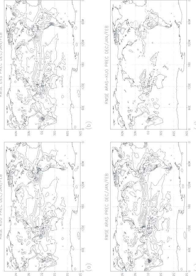
Figure 7 - Root mean square error (RMS) of climatological precipitation for december, January and February. (a) KUO, (b) ARAS, (c) KUO+ARAS and (d) ARAS-KUO. Intervals are 2 mm.day-1.
KUO, also seen in other regions. Considering the difference between observed and simulated precipitation, although there is overestimation in both results, ARAS scheme produced better results comparatively to KUO scheme in SE region (4.22 mm.day-1 in KUO and 1.59 mm.day-1 in ARAS). In the Amazon area (c), the difference between observed and simulated precipitation using KUO (0.18 mm.day-1) was smaller than using ARAS (2.70 mm.day-1). Over central South America (e), both KUO and ARAS underestimate the precipitation and
KUO scheme shows more consistency among the members (STd =1.10 mm.day-1) compared to ARAS (STd=1.68 mm.day-1). Over Nordeste (a), the differences between model and observations, and the standard deviation among members are smaller with KUO. In this region, ARAS underestimates the precipitation (-1.05 mm.day-1), while KUO scheme overestimates (0.31 mm.day-1) Southern Brazil and Argentina
Figure 9 - Omega zonal mean (latitude-level). (a) KUO, (b) ARAS, (c) NCEP reanalysis.
regions the standard deviations among the membersare similar and small considering both schemes. Simulated precipitation using ARAS scheme over the Paciic area is very similar to the observations (k), while in the KUO scheme the values are overestimated. Over the Atlantic, both schemes show large differences and KUO scheme presents the largest errors.
Table 3 presents the observed precipitation (mm.day-1)
ensemble (KUO +ARAS), the results are slightly improved over some areas such as southern Northeast (b) and Argentina (i-j). A larger improvement in the ENS is seen over the Paciic area (k) where the smallest error occurs, only 1%. The monthly results of each integration, for each area, considering both experiments and the observations are displayed in Figure 14. Both schemes show convergence among members in Northern
Nordeste (a), Amazon region (c), southern Argentina (j) and over the oceans (k-l). Lesser degrees of convergence are seen in southern Brazil, Uruguay and Argentina/Paraguai (g-h) and northwest of Peru and Ecuador (f). Larger dispersion is seen in the southern Northeast (b), Southeastern Brazil (d), Central South America (e) and northern Argentina (i). The results suggest that tropical and extratropical South America are not
Figure 10 - Zonal mean vertical proile of zonal wind for December, January and February. (a) KUO, (b) ARAS, (c) KUO+ARAS and (d) NCEP
Figure 11 - Root mean square error (RMS) of zonal wind ield zonal mean for December, January and February. (a) KUO, (b) ARAS and (c)
ARAS-KUO. Interval is 1 m.s-1.
dependent of the initial conditions, being affected directly mainly by large-scale SST forcing conditions (tropics) and by frequent passages of synoptic systems (extratropics). On the other hand, the areas of southeastern Brazil, southern Northeast and central South America, which are affected by the South Atlantic Convergence Zone (SACZ), are very dependent on the initial conditions. Northern Argentina seems to have a particular
behavior, different from southern and eastern Argentina.The different dependence on the initial conditions in these regions may be related to different trajectories of the synoptic systems over South America. Some can move from southwestern South America northward, along the coast, or can propagate to the interior of the continent, and some can be displaced to the ocean (Andrade, 2007). Thus, different results in the areas
a)
b)
Figure 12 - difference of wind magnitude at 200 hPa between
model simulations and re-analysis wind ields. (a) KUO minus NCEP
reanalysis, (b) ARAS minus NCEP reanalysis and (c) KUO+ARAS
minus NCEP reanalysis. Interval is 3 m.s-1.
can be associated with the different behavior of the systems in each integration over South America. Although the spatial maps show errors in both schemes, when the analysis is performed regionally (Figure 14), it is seen that the observed precipitation over northern Nordeste and Amazon region (magnitude and monthly variation) are very well simulated by the model when KUO scheme is used, and the results with ARAS are far from the observations. In these regions the two ensembles are well separated. Over northern and southern Argentina, southern Brazil, Uruguay and Argentina, the results of both KUO and ARAS are mixed. This is consistent with precipitation that is not associated with deep convection in extratropical regions. Over the Paciic Ocean, the ARAS results are closer to observations than KUO. This result is consistent with those showed by Kirtman and deWitt (1997) where they found a better simulation of winds over Paciic Ocean using the ARAS scheme.
7. CONCLUDING REMARKS
In this study two convection schemes, KUO and a modiied version of Arakawa-Schubert (ARAS), are applied to the CPTEC/COLA AGCM in two sets of ive integrations, in order to analyze the climatological response of the model with respect to precipitation over South America and to some atmospheric global and regional features. The results have shown that the KUO scheme gives smaller precipitation magnitude errors than the ARAS scheme in 7 out of 12 analyzed areas, representing 64% of the total areas. ARAS scheme shows smaller errors than KUO scheme over tropical Atlantic and Paciic oceans, Southeast, Uruguay and part of eastern Argentina. In most of land areas, precipitation is best simulated by KUO. However, ARAS scheme reduces the errors in the southern area of the SACZ over the eastern coast of Brazil, where the KUO scheme shows the largest errors. A combination of both schemes improves the precipitation ield coniguration over northern Northeast Brazil, northwestern Amazon and southern part of the SACZ, but still resulting in large errors in the central part of the band which is displaced northwards of the observed position.
Concerning the large-scale atmospheric characteristics in the Southern Hemisphere, both schemes have shown errors at high latitudes linked to errors in the jet stream intensity and position. A combination of both schemes seems to improve the results of wind and geopotential ields. The ARAS scheme improves the vertical zonal wind structure at upper levels of North Hemisphere but worsen in all levels of the South Hemisphere.
Table 2 - Statistics for the selected averaged areas. First column indicates the area. Second, third, fourth and ifth columns show the precipitation
simulated when KUO scheme is used, precipitation minus observations, RMS and standard deviation of each member relatively to the ensemble mean of this scheme, respectively. Sixth, seventh, eighth and ninth columns show the precipitation simulated when ARAS scheme is used, precipitation minus observations, RMS and standard deviation of each member relatively to the ensemble mean of this scheme, respectively. The remaining columns show the precipitation simulated when the total ensemble mean (ENS) is considered, ENS minus observations, RMS and standard deviation of each member relatively to the total ensemble mean, respectively. All units are in mm.day-1.
Table 3 - Statistics for the selected averaged areas. First column indicates the area. Second, observed precipitation (CMAP), third column is the
percentage of error when KUO scheme is used, fourth is the percentage of error when ARAS scheme is used and ifth when the total ensemble mean
Pezzi and Kayano (2007). The use of a superensemble where different weights are given to different models with different schemes have reduced errors and improved the simulations. The Grell ensemble scheme (Grell et al., 2002) for deep convection is being tested at CPTEC in the AGCM, and preliminary results show improvements in the summer precipitation ield over
South America. Other schemes should also be tested, such as the mass lux used by the Hadley Centre (Gregory and Rowntree, 1990). This scheme has been used in HadC3 climate simulation (Johns et al. 1997) and it was noticed that the precipitation over South America was closer to the observations than other models (Cavalcanti et al. 2002).
Figure 13 - South America areas for the analysis of monthly spatial averaged precipitation considering model experiments and CMAP data. (a) Northern Nordeste, (b) Southern Nordeste, (c) Amazon, (d) Southeast Brazil, (e) Central South America, (f) Northwest Peru and Ecuador, (g) Southern Brazil, Uruguay and eastern Paraguay, (h) Southern Brazil, Uruguay and Eastern Argentina, (i) Northern Argentina, (j) Southern Argentina,
8. ACKNOWLEDGMENTS
We would like to thank dr. Pedro Leite da Silva dias and dr. Silvio Nilo Figueroa for discussions about the cumulus convection parameterization adjustments. We would also like to thank an anonymous reviewer for the comments, which relected on substantial improvements to the paper. The second author thanks CRN-O55 (IAI project). We also thank CNPq and FAPESP for supporting our research activities.
9. REFERENCES
ANTHES, R. A. A cumulus parameterization scheme utilizing a one- dimensional cloud model. Mon. Wea. Rev., v. 105, n. 3, p. 270-286, 1977.
ARAKAWA, A. and W. H. SCHUBERT. Interaction of cumulus cloud ensemble with large-scale environment. Part I. J. Atmos. Sci, 31,671-701, 1974.
BETTS, A. K. and M. J. MILLER. The Betts-Miller scheme. The representation of Cumulus convection in numerical models, Metor. Monogr. N46. K. A. Emanuel and d.J. Raymond, Eds., Amer. Meteor. Soc., 107-122, 1993.
CAVALCANTI, I. F. A.; J. A. MARENGO; P. SATYAMURTY; C. A. NOBRE; I. TROSNIKOV; J. P. BONATTI; A. O. MANZI; T. TARASOVA; C. D’ALMEIDA; G. SAMPAIO; L. P. PEZZI; C. C. CASTRO; M. SANCHES; H. CAMARGO. Global climatological 21 features in a simulation using CPTEC/COLA AGCM. J. Clim., 15, 2965-2988, 2002.
CAVALCANTI, I. F. A.; J. A. MARENGO; C. C. CASTRO; G. SAMPAIO; M. SANCHES. Climate prediction of precipitation over South America for dJF 1999/2000 and MAM 2000 using the CPTEC/COLA AGCM. Exper. Long-Lead For. Bull., 8, (4), 43-46, 1999.
dE WITT d.G. The Effect of the Cumulus Convection on the Climate of the COLA General Circulation Model. Cola Tec. Rep., 27, 1996.
GRAHAM, N. E. Prediction of rainfall in Northeast of Brazil for MAM 1994 using an atmospheric GCM with persisted SST anomalies. Exper. Long- Lead For. Bull., 1994. GREGORY, D., P. R. ROWNTREE, 1990: A mass
° u x c o n v e c t i o n s c h e m e w i t h r e p r e s e n t a t i o n of ensemble characteristics and stability dependent closure. Mon. Wea. Rev., 118, 1483-506, 1994 GRELL, G. A., DEVENYI, D. A generalized approach
to parameterizing convection combining ensemble and data assimilation techniques. Geophys. Resear. Lett., (29)-14, 10.1029/2002GL015311, 2002. JOHNS, T. C., R. E. CARNELL, J. F. CROSSLEY, J. M.
GREGORY, J. B. MITCHELL, C. A. SENIOR, S.
B. TETT, R. A. WOOd. The second Hadley Centre coupled ocean-atmosphere GCM: model description, spinup and validation. Clim. Dyn., (13), 103-134, 1997. KALNAY, E. M ET AL.. The NCEP/NCAR 40-Year Reanalysis
Project. Bull. Amer. Meteor. Soc., (77) 437-471, 1996. KINTER, J. L., D. DE WITT, P. A. DIRMEYER, M.
J. FENNESSY, B. P. KIRTMAN, L. MARX, E. K. SCHINEIdER, J. SHUKLA, and d. STRAUS. The COLA Atmosphere-Biosphere General Circulation Model Volume 1: Formulation. Cola Tech Rep., 51(1) 46pp, 1997. KIRTMAN, B. P. and d. dE WITT. Comparison of atmospheric
model wind stress with three different convective parameterisations: Sensitivity of Tropical Paciic Ocean simulations. Mon. Wea. Rev., (125) 1231-1250, 1997. KOUSKY, V. E., M. T. KAYANO, I. F. A. CAVACALTI.
A Review of the Southern Oscillation: Oceanic-a t m o s p h e r i c c i r c u l Oceanic-a t i o n c h Oceanic-a n g e s Oceanic-a n d r e l Oceanic-a t e d rainfall anomalies. Tellus, 36A 490-504, 1984. KRISHNAMURTI, T.N., C.M. KISHTAWAL, d.W.
SHIN and C.E. WILLIFORd. Improving Tropical P r e c i p i t a t i o n F o r e c a s t s f r o m a M u l t i a n a l y s i s Superensemble J. Clim., 13 4217-4227, 2000. KRISHNAMURTI, T.N., S. SURENdRAN, d.W. SHIN,
R. CORREA-TORRES, T.S.V. VIJAYA KUMAR, C.E. WILLIFORd, C. KUMMEROW, R.F. AdLER, J. SIMPSON, R. KAKAR, W. OLSON and F.J. TURK. Real Time Multianalysis/Multimodel Superensemble Forecasts of Precipitation using TRMM and SSM/I Products. Mon. Wea. Rev., 129, 2861-2883, 2001. KUO, H. L. On the formation and intensification
of tropical cyclones through latent heat release by cumulus convection. J. Atmos. Sci., (22) 40-63, 1965. MARENGO, J. A., I. F. A. CAVALCANTI, P. SATYAMURTY,
I. TROSNIKOV, C. A. NOBRE, J. P. BONATTI, H. CAMARGO, G. SAMPAIO, M. B. SANCHES, A. O. MANZI, C. A. C. CASTRO, C. d’ALMEIdA, L. P. PEZZI and L. CANdIdO. Assessment of regional seasonal rainfall predictability using the CPTEC/COLA atmospheric GCM. Clim. Dyn, 21(5-6) 459-475, 2003. MOORTHI, S. and M. J. SUAREZ. Relaxed Arakawa-Shubert:
A parameterizetion of moist convection for general circulation models. Mon. Wea. Rev., 120, 978-1002, 1992. NOBRE, P. and J. SHUKLA. Variations of sea surface
temperature, wind stress and rainfall over the Ttropical Atlantic and South America. J. Clim., 10(4) 2464-2479, 1996. PEZZI, L. P. and I. F. A. CAVALCANTI. The Relative
drought in Northeast Brazil. Int. J. Clim., 6(1) 43-51, 1986. REYNOLDS, R. W. and T. M. SMITH. Improved g l o b a l s e a s u r f a c e t e m p e r a t u r e a n a l y s e s u s i n g optimum interpolation. J. Clim., (7) 929-948, 1994. R O P E L E W S K Y, C . F. a n d M . S . H A L P E RT.
Quantifying southern oscillation - precipitation relationships. J. Clim., (9) 1043-1059, 1996. SILVA-dIAS, P. L. Experiments with the Arakawa-Schubert cumulus Parameterization theory. Ph. D.Thesis, Colorado State University, 132 pp., 1977. SOUZA, E., KAYANO, M. T., TOTA, J., PEZZI, L., FISCH,
G. and NOBRE, C. On the Inluences of the El Nino, La Nina and Atlantic dipole Pattern on the Amazonian Rainfall During 1960-1998. ACTA Amazonica, 30(2) 305-318, 2000.
SPERBER, K., and PALMER, T. Interannual tropical rainfall variability in general circulation model simulations associated with the Atmospheric Model Intercomparison Project. J. Clim., 9, 27272750, 1996. SUD, Y. and MOLOD, A. The roles of dry convection, cloud
radiation feedback processes, and the inluence of recent improvements in the parameterization of convection in the GLA GCM. Mon. Wea. Rev., v. 116, n. 11, 2366-2387, 1988. VASUBANDHU, M., DIRMEYER. P. A. and KIRTMAN,
B. P. dynamic downscaling of seasonal simulations over South America. J. Clim., v. 116, n. 1, p. 103-117, 2003. XIE, P. and ARKIN, P. Analyses of global monthly precipitation