0103 - 5053 $6.00+0.00
Article
*e-mail: [email protected]
Atmospheric Corrosion Performance of Carbon Steel, Galvanized Steel, Aluminum
and Copper in the North Brazilian Coast
Yuri C. Sica,a Elaine D. Kenny,a Kleber F. Portella*,a and Djalma F. Campos Filhob
a
Instituto de Tecnologia para o Desenvolvimento, CP 19067, 81531-980 Curitiba-PR, Brazil
b
Centrais Elétricas do Norte do Brasil, 65095-530 São Luís-MA, Brazil
Para a caracterização, classificação e o mapeamento da corrosividade atmosférica da cidade de São Luís-MA, região costeira do Norte do Brasil, foi desenvolvida uma metodologia baseada na implantação de quinze estações de corrosão atmosférica (ACS) abrangendo diferentes ambientes corrosivos. Nestas ACS foram monitorados, mensalmente, a taxa de deposição dos principais poluentes atmosféricos (íons cloreto, Cl–; gases compostos de enxofre, expressos em SO2 e partículas sedimentáveis) e os parâmetros meteorológicos, a fim de se obter subsídios para a classificação da corrosividade atmosférica. Em quatro destas ACS foram instalados, além dos módulos de coleta de poluentes, painéis de intemperismo natural com corpos-de-prova dos materiais metálicos: aço-carbono, aço galvanizado, alumínio e cobre, metais mais utilizados no setor de distribuição e transmissão de energia elétrica local. Da classificação atmosférica foi elaborado mapa para promover a seleção dos materiais segundo seu desempenho em cada região e diminuir custos diretos e indiretos da corrosão pela extensão da sua vida-útil.
The main purpose of this study is to develop a method to characterize and classify the atmospheric corrosivity of the Sao Luis City, located at the Brazilian North coast, establishing 15 atmospheric corrosion sites (ACS), in different environments. These sites were monitored on a monthly basis to determine the deposition rates of atmospheric contaminants, such as airborne salinity, represented by chloride ions (Cl–), sulfur-containing substances, represented by SO2 and dustfall. These parameters were correlated to meteorological data and both were used to classify the atmospheric corrosivity. At the same time, metallic samples such as low carbon steel, galvanized steel, aluminum and copper, which are commonly used in transmission and distribution power lines, were exposed to the environment in four of these 15 sites, in order to qualify the environmental aggressiveness according to the corrosion rate of these materials. Based on the mapping results, it was possible to determine the materials which are more proper to be used in those specific areas, which could result in the cost reduction due to a span-life extension of such structures.
Keywords: atmospheric corrosion, metals degradation, corrosion mapping
Introduction
The industrial development during last decades has brought a significant evolution for the installations, equipments and metallic and non-metallic structures exposed to the atmosphere. The air has also become more polluted and therefore more aggressive to the materials exposed to a great quantity of gases, reagents and chemical vapors released into the atmosphere as also in soils, rivers and the sea.
The quantity of contaminants may vary due to the proximity of the emitting sources and to the climate
conditions such as temperature, rain, relative humidity, solar radiation and pressure.1 The wind vertical direction affects
the climate and the important synergetic processes related to environmental pollution.2 The short vertical motion is
called “stable” and the long is known as “unstable”. The wind speed is other important factor for the pollutants dispersion and may act as a vehicle for the erosion corrosion, mainly in environments with high particles contents. For these reasons, it is important to study the meteorological influence in atmospheric corrosion.
Examples are most of the engineering products, the electricity transmission lines and cables, the transportation means, most of the electricity towers and telephone lines, car and pedestrian overpasses, bridges, pipelines storing tanks, among many others.3
All the phenomena that influence the kinetic of atmospheric corrosion processes can be divided in macroclimatic and microclimatic. Water precipitation (rain, snow or mist), humidity condensation due to temperature changes (dew) allied to the solar radiation and the chemical composition of atmosphere (air contamination by gases, acid vapors and sea aerosols) are the main factors responsible for the atmospheric corrosive ability and define the macroclimate of the region.4,5 On the other hand, the microclimate is defined
by the electrolyte layer formed over the metal surface, which influences the corrosive processes that are essentially electrochemical. Among the parameters that define the microclimate, it can be considered: i) wetness time; (ii) the heating of metallic materials when exposed to solar radiation, especially to infrared light; and (iii) other kinds of chemical pollution (SO32–; NO
x, Cl –,
industrial dust, organic acids, etc).6
The wetness time (τ) can be estimated by the binomial temperature-relative humidity, that is the time to the ambient air to reach 80% RH at any temperature (T) > 0 ºC.7-11 From the correlation of these parameters to the metal
corrosion rate, it is possible to classify the environmental corrosivity degree, in 5 categories. It is based on sulfur-containing substances represented by SO2 (P), airborne salinity represented by chloride (S), and the corrosivity (C) index by the wetness time (τ).5,7,11 In Table 1, it is
presented the classification of the environment in corrosivity categories.
Tables 2 and 3 show some of the main physicochemical parameters used to classify the environment in accordance to corrosion rates and corrosivity to metal or alloy.
In this work, samples of low carbon steel, galvanized steel, aluminum and copper plates used in electricity distribution and transmission lines were studied. The materials were classified in corrosive categories, according to Table 4. The international standard ISO 9223 recommends
the use of metallic zinc samples with a minimum purity of 98.5% of zinc as standard.7 However, it was used galvanized
steel samples constituted by carbon steel substrate recovered by zinc, coated by the hot dip immersion process. This choice was based on its large utilization as metallic structures in electricity distribution and transmission systems.
Experimental
For the classification of the atmospheric corrosivity and its effect on the studied materials (SM - carbon steel, galvanized steel, aluminum and copper), data was collected from all the 15 atmospheric corrosion sites (ACS) located in different areas of the Sao Luis City -Brazil, in order to study the very aggressive environment, due to the salinity and industrial pollutants, and the less aggressive regions, far from the seashore or industrial complexes. The following parameters were monitored: sulfur-containing substances, airborne salinity in marine atmospheric represented by chloride, dustfall deposition rate, temperature, RH%, wetness time (τ), global radiation, wind speed and direction. The corrosivity rates of the samples were measured considering the lifetime of the metals during the experiment.
Monitored regions
In the Northern part of Sao Luis Island, 10 ACS were placed, as well as 5 in the South part, these later corresponding to the Southern and continental industrial
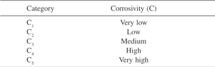
Table 1. Categories of corrosivity of the atmosphere11
Category Corrosivity (C)
C1 Very low
C2 Low
C3 Medium
C4 High
C5 Very high
Table 2. Classification of the environment in terms of τ, sulfur-contain-ing substances (P) and airborne salinity (S)7
Category τ/ SO2 / (P) Cl– / (S)
(h/year) (mg per m2 a day) (mg per m2 a day)
τ1; P0; S0 ≤10 ≤10 ≤3
τ2; P1; S1 10 – 250 10 – 35 3 – 60
τ3; P2; S2 250 – 2500 35 – 80 60 – 300
τ4; P3; S3 2500 – 5500 80 – 200 300 – 1500
τ5 > 5500 > 200* > 1500*
Note: * estimated values.
Table 3. Classification of corrosivity of the atmosphere according to Liesegang12
Corrosive Atmospheric contamination
environment SO3 / (mg per SO2 calculated / Cl– / (mg 100 cm2 a day) (mg per m2 a day) per m2 a day)
1. Rural 0.12 – 0.37 9.6 – 29.6 < 30 2. Urban 0.37 – 1.25 29.6 – 100.0 < 30 3. Industrial 1.25 – 2.50 100.0 – 200.0 < 30 4. Marine 0.12 – 0.37 9.6 – 29.6 30 – 3000 5. Industrial
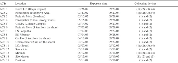
complexes, according to the illustrative map in Figure 1. In Table 5, the collecting device type and the exposure time for each ACS are listed. The devices at ACSs 1 to 10 were connected to the poles, located as high as the electricity lines and the devices at ACSs 11 to 15 were connected to the transmission towers (TL 500 kV “Presidente Dutra” transmission power line, 200 km long), installed 15 meters high from the ground.
The ACS locations were defined by the local Energy Company, as a function of the places with a large number of energy breakdowns caused by the high corrosivity to
the materials and to the high maintenance costs of the electricity network.
Climate classification of a determined region
As it was already verified,4 high RH% and temperature
values improve the degradation process of the materials in the atmosphere. Based on such concept, Brooks apud Morcillo et al.5 presented an index for the corrosive
potential, based on meteorological data.The numeric value was named Brooks’ deterioration index (Id) and it is calculated from the vapor pressure (obtained expe-rimentally or from standard tables)13 at the temperature
and RH% on the region. According to the Id value, the corrosion rates have a direct correlation with the environment corrosivity as illustrated in Table 6.
Determination of the chloride deposition rate
The determination of the airborne salinity represented by chloride deposition rate in the atmosphere (soluble chlorides as those from the industrial or marine atmosphere aerosols) was carried out in accordance with NBR 6211 which prescribes the moist candle method.14 The results
are expressed in mg of Cl–per m2 a day.
Determination of the sulfate deposition rate
The determination of the sulfate deposition rate was carried out in accordance with NBR 6921, which prescribes the gravimetric determination of sulfate deposition rate in the atmosphere obtained by the oxidation or fixation of sulfur-containing substances (SO2, SO3, H2S and SO42–) on a reactive surface.15 The results are expressed
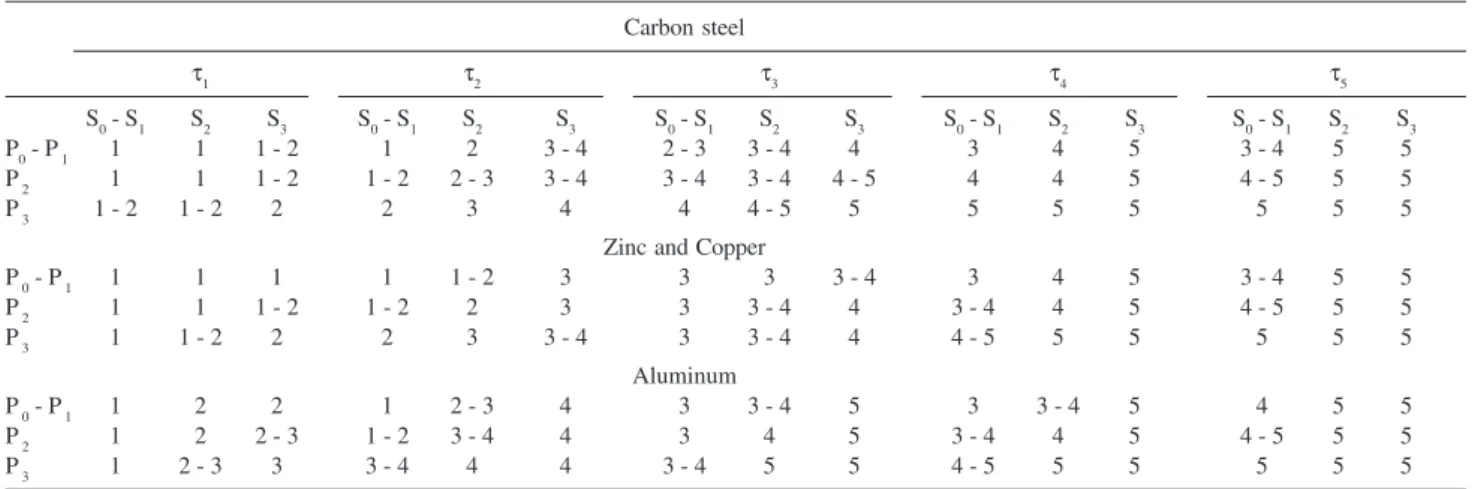
in mg of SO2per m2 a day. Table 4. Estimated corrosivity categories of the atmosphere for standard metals11
Carbon steel
τ1 τ2 τ3 τ4 τ5
S0 - S1 S2 S3 S0 - S1 S2 S3 S0 - S1 S2 S3 S0 - S1 S2 S3 S0 - S1 S2 S3
P0 - P 1 1 1 1 - 2 1 2 3 - 4 2 - 3 3 - 4 4 3 4 5 3 - 4 5 5
P 2 1 1 1 - 2 1 - 2 2 - 3 3 - 4 3 - 4 3 - 4 4 - 5 4 4 5 4 - 5 5 5
P 3 1 - 2 1 - 2 2 2 3 4 4 4 - 5 5 5 5 5 5 5 5
Zinc and Copper
P 0 - P 1 1 1 1 1 1 - 2 3 3 3 3 - 4 3 4 5 3 - 4 5 5
P 2 1 1 1 - 2 1 - 2 2 3 3 3 - 4 4 3 - 4 4 5 4 - 5 5 5
P 3 1 1 - 2 2 2 3 3 - 4 3 3 - 4 4 4 - 5 5 5 5 5 5
Aluminum
P 0 - P 1 1 2 2 1 2 - 3 4 3 3 - 4 5 3 3 - 4 5 4 5 5
P 2 1 2 2 - 3 1 - 2 3 - 4 4 3 4 5 3 - 4 4 5 4 - 5 5 5
P 3 1 2 - 3 3 3 - 4 4 4 3 - 4 5 5 4 - 5 5 5 5 5 5
Note: Corrosivity is expressed by the numeric part of the corrosivity category code (for example: 1 instead of C1).
Determination of dustfall rate
The determination of dustfall rate was carried out in accordance to ASTM D1739.16 This method prescribes
the collecting of atmospheric dust in large areas by the determination of soluble and non-soluble particulates materials. The dust is collected in a polymeric material recipient with an upper cover and known internal area and volume. The results are expressed in g per m2 in 30
days of settleable particulate matter in the atmosphere.
Performance assessment of the metallic materials exposed to natural weathering
The SM (carbon steel, aluminum, copper and galvanized steel) were placed over panels located in some of the ACSs, in order to improve the evaluation of the micro and macroclimate variables of the local atmospheric corrosion. The chosen places are indicated as collecting device number 4 in Table 5.
The panels were installed in accordance to NBR 620917
with some modifications, as follows: ACS 1 panel was positioned to the North-East direction facing the I.C. close to the sea; ACS 2 panel was installed facing the geographic North in order to receive more sunlight on the metallic surfaces, as recommended in the methodology; the ACSs
11 and 13 panels were installed in the transmission line towers, the former being faced to a South I.C. complex and the latter to the geographic North. All the plates were always faced to an environment with the greatest wind and solar radiation incidence, as well as atmospheric pollutants.
The wind direction and speed were important parameters to be considered when choosing the places because of their straight influence on the dispersion and synergism of the pollutants.
Sheet plates with (5 × 10) cm2 in size and 0.3 cm in
thickness of all MSs were prepared in accordance to NBR 6210.18 All MSs were identified by manual punching. Table
7 lists the exposed MSs in the respective ACSs, as well as the number of corrosion rate tests for the different metals. After each 30-day exposition and previous visual inspections (all registered on photographs), a specific cleaning for the corrosion products removal was carried out, according to the type of each standard metallic plate. Such procedure was done by mechanical and chemical processes, taking care not to remove the substrate or the coating metallic materials. After this cleaning, the MSs that had presented uniform corrosion were weighed for the mass loss and corrosion ratedetermination.19,20 Table 5. ACS collecting modules installed in Sao Luis City
ACSs Location Exposure time Collecting devices
ACS 1 North I.C. (Itaqui Region) 03/26/02 09/27/04 (1); (2); (3); (4)
ACS 2 Renascença (Mangrove Area) 03/27/02 09/27/04 (1); (2); (3); (4)
ACS 3 Praia do Meio (Seashore) 05/15/02 09/28/04 (1) and (2)
ACS 4 Panaquatira (Shore; strong winds) 05/15/02 09/28/04 (1) and (2)
ACS 5 UEMA (College Campus) 05/14/02 09/27/04 (1) and (2)
ACS 6 Praia do Meio (1 km from the shore) 07/02/03 09/28/04 (1) and (2)
ACS 7 ES Forquilha 07/07/03 09/27/04 (1) and (2)
ACS 8 ES Ribamar 07/04/03 09/28/04 (1) and (2)
ACS 9 Caolho (1 km from the shore) 04/12/04 09/28/04 (1) and (2)
ACS 10 Urban center (2 km off the shore) 04/12/04 09/27/04 (1) and (2)
ACS 11 I.C. (South) 05/07/04 05/12/05 (1); (2); (3); (4)
ACS 12 Santa Rita 05/11/04 05/12/05 (1) and (2)
ACS 13 Miranda 05/12/04 05/11/05 (1); (2); (3); (4)
ACS 14 São Mateus 05/13/04 05/10/05 (1); (2) and (3)
ACS 15 Peritoró 05/13/04 05/10/05 (1) and (2)
Note: I.C. and ES correspond to the data collection near to the industrial complex and to the electrical energy substation, respectively; (1) chloride device; (2) sulfate device, (3) dustfall device and (4) natural weathering panel.
Table 7. Identification of the MSs exposed in the ACSs
ACS MS code Material/Coating Number of corrosion rate tests
ACSs 1 and 2
S Carbon steel 6
A Aluminum 4
C Copper 5
G Galvanized steel 4
ACSs 11 and 13
S Carbon steel 8
A Aluminum 8
C Copper 8
G Galvanized steel 8
Table 6. Deterioration index (Id) of Brooks5
Id Corrosion rate Id Corrosivity
Id < 1 Very low 0 – 1 no corrosive
1 < Id < 2 Low 1 – 2 very low corrosive 2 < Id < 5 Medium 2 – 4 a bit corrosive
Id > 5 High 4 – 5 corrosive
After checking the evidence of localized attack, the aluminum and copper surfaces were investigated with a SMZ800 NIKON stereoscopic microscope for the corrosion type, and by metallographic analysis using a MM6 Leitz-Wetzlar optical microscope (OM). The samples for the metallographic tests were cut and set with bakelite, sandpapered up to 1200 granule and polished with 3 µm diamond-paste.
Meteorological parameters and classification of corrosivity atmosphere degree
The meteorological parameters (temperature, RH%, precipitation, solar radiation, direction and speed of the wind) were obtained from previous information supplied by CPTEC – Centro de Previsão de Tempo e Estudos Climáticos (Climate Studies and Weather Forecast Center),21 essential for the classification and
charac-terization of the atmospheric corrosion.7,11
For the climatic classification of Sao Luis City, two methodologies were used: Köppen and Strahler apud
Morcillo et al.5 The Köppen5 methodology presents five
climate types which classify the Brazilian territory based on temperature and annual average pluviosity, as follows: Am – equatorial; Aw – tropical; Bsh – semi-arid; Cwa – tropical of altitude and Cf – subtropical. Köppen apud
Morcillo et al.5 is based also on the main dynamic systems
of atmospheric mass circulation in Brazil: Atlantic equatorial mass (aEm) and continental equatorial mass (cEm); Atlantic tropical mass (aTm) and continental tropical mass (cTm) and, finally the Atlantic polar mass (aPm). The Strahler apud Morcillo et al.5 climate
classification proposes that the climates in the Brazilian territory can be controlled by tropical-equatorial and polar-tropical air masses and divides the atmosphere, like Köppen apud Morcillo et al.,5 in five climatic types: humid
equatorial climate (convergence of the trade winds); humid coastal climate (influenced by aTm); alternating humid and dry tropical climate; semi-arid tropical climate and humid subtropical climate.
Atmospheric corrosivity mapping
For the corrosivity mapping it was used a local environmental data bank (meteorological and pollutants) during the period of study and the corrosivity categories are expressed in Table 4,11 using the average values
corresponding to the more critical period (from July to December). These data were georeferenced by a geoprocessing software – ArcView 9.0 GIS (Geographic Information System) developed by ESRI, in which the
vectorial and punctual layers were defined in order to be interpolated by the deterministic interpolating method, called Inverse Distance Weighed (IDW). This method is a geospatial analysis resource available on the ArcView 9.0’s Spatial Analyst. It is based on the combination of the corrosivity rate group determined for each ACS in which the pondering factor is reversed to the distance and which provides a continuous surface, named atmospheric corrosivity raster.12, 22
Results and Discussion
Meteorological data
Based on the literature,4,5 and referring to the
atmospheric circulating dynamics, the climate of Sao Luis City is controlled by the tropical and equatorial air masses. According to the climatic classification of Strahler apud Morcillo et al.,5 the Maranhao State –
Brazil may be considered between the alternate humid/ dry tropical and humid equatorial climates. It has the influence of the Atlantic equatorial mass (aEm), which has its origin center in the Atlantic Ocean. In the summer, this climate is dominated by the continental equatorial mass (cEm) with its origin center in the Western part of the Amazon region, which leads to frequent rains. Due to the contact between trade winds, most of the precipitation is in the convectional form. Rains are abundant and the dry season is relatively short. Although such continental air masses are usually dry, the cEm is hot and humid because of the Amazon forest and also for the large number of rivers in the region.
Based on the meteorological data available from 2002 to 2005, it can be confirmed that the region of Sao Luis City is settled between the equatorial Am and tropical -Aw climates, according to Köppen apud Morcillo et al.,5
being characterized by two defined seasons: the dry period (July to December) and the rainy period (January to June). In Figure 2, the monthly averages are presented for the meteorological parameters of accumulated precipitation, RH% and temperature of the period from 2002 to 2005 for the Sao Luis City. It stands out the dry period that goes between July and December and the seasoned behavior.
It is observed that the annual average temperature of Sao Luis is around (28 ± 4) ºC.21 The atmosphere of the
of the ions from the atmosphere, mainly Cl– and SO 4
2–
coming from the sea wind air,12 and the contact with the
metal surfaces. On the other hand, the rain which is usually responsible for the leaching of the atmospheric pollutants, may also decrease the electrolyte concentration and also the corrosion rate.
The average accumulated solar radiation for the rainy period is about 672 MJ m-2, and the highest value
for the dry period about 1027 MJ m-2.21 This fact
influences both the τ on the metal and the corrosion rate, due to the semi-conducting behavior of the oxidative corrosion processes.6
North-East trade wind is predominant, with an average speed of 6.3 m s-1.21 It influences the dispersion and the
synergy of the atmospheric pollutants and the electrolyte drying time of the metal surface.
In accordance with NBR 14643,11 the calculated t of
approximately 4400 hours for the assessed period leads the classification of Sao Luis City atmosphere to the τ4
corrosivity category, which is classified as high corrosive atmosphere. The RH% condition higher than 70%, allied to annual average temperatures near to 30 ºC leads to deteriorating processes of materials in air, especially metals. This deteriorating index of atmosphere (Id), obtained from Brooks expression was 4.7 for the City of Sao Luis, classified as corrosive with moderate deterioration degree.
The high tendency to corrosion and abrasion-erosion processes on the surface of the materials, observed during the visual inspection on the metallic components of the electric energy distribution towers placed along the seashore, corroborates with the North-East direction of the predominant winds.
Chloride deposition rate
The chloride deposition rates, shown in Figure 3, are more expressive than the sulfur dioxide ones, shown in Figure 4, due to the proximity to the seashore. It may also be observed that in the ACSs 3 and 4 it was obtained chloride average rate values of 380 and 290 mg per m2 a
day, respectively. This is explained due to their proximity to the seashore when compared to any other ACS. As the RH% values were higher than 70%, the chloride ions were surely in the degradation process of the metallic materials since they are highly hygroscopic and strong electrolytes. From the former results, the environmental corrosivity degree for each ACS can be ordered as follows:
ACS 3 > ACS 4 > ACS 1 > ACS 6 > ACS 8 > ACS 2 > ACS 7 > ACS 11 > ACS 10 ≅ ACS 12 > ACS 13 ≅ ACS 9 > ACS 5 > ACS 14 ≅ ACS 15
Figure 2. Accumulated precipitation, temperature and RH% curves (monthly average values), between 2002 and 2005 in the City of São Luis - Brazil.
Figure 3. Average atmospheric chloride deposition rates for each ACS during the studied period.
Sulfur dioxide deposition rate
The SO2 deposition rate for each ACS is presented on Figure 4. This parameter was significant for the environmental corrosivity classification. The ACS stations are considered as typically rural environments from the Liesegang apud Kenny et al. classification.12 However,
the total sulfate deposition rates, even with lower values, followed the seasoned chloride quantities.
In ACSs 3 and 4, just like for the chloride quantities, sulfate deposition is higher than the others, probably because of the sulfate particle dragging. It is a consequence of the sea-wave splashing and of the winds. In general the values were considered low, with rates between 9.60 and 29.61 mg of SO2 per m2 a day. In such value range, the
local environment may be classified as a marine-rural corrosivity place.12 From these results, the environmental
corrosivity degree for each ACS also can be ordered:
ACS 4 ≅ ACS 3 > ACS 7 > ACS 1 > ACS 6 > ACS 0 > ACS 9 ≅ ACS 11 ≅ ACS 2 ≅ ACS 8 > ACS 5 > ACS 13 ≅
ACS 14 ≅ ACS 15
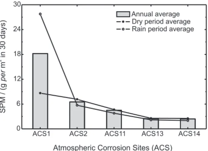
Settleable Particulate Matter (SPM)
The dustfall quantities measured at 5 ACSs installed in Sao Luis City are shown in Figure 5. The importance of this parameter is related not only to its concentration but also to its form and chemical composition. Solid particles, in dust and soot forms, are responsible for increasing the atmosphere corrosivity due to their hygroscopic properties. A typical case is the amorphous silica, which has the ability to retain humidity and to favor the electrochemical corrosion, leading to a localized corrosion.12 The same fact is observed with
metallic particles such as iron and aluminum, which can
aggravate the corrosive process when their chemical nature is different from the base metal (galvanic corrosion process).3
The form and the chemical composition of the particulate materials were not focused in this work.
From the results, it was possible to verify that ACS 1 had the higher dustfall rate, mainly during the rainy period, followed by ACS 2. Both are next to the seashore and to industrial complexes. ACS 11, 13 and 14 presented low dustfall rates, once they are installed at about 15 meters high in a rural environment.23
Comparing the regions, it was possible to classify the ACSs in the following decreasing order:
ACS 1 >> ACS 2 > ACS 11 > ACS 13 ≅ ACS 14
Pursuing the atmospheric pollutants quantity shows that the chloride ion amount, the annual average temperature of 28 ºC and a τ >45%, are the main factors for the observed high corrosivity at the ACSs installed in Sao Luis City. It is important to consider that the greatest rates of atmospheric chlorides and sulfates deposition were recorded in the dry period (July to December), in which the pollutant wash-away did not occur.
Natural weathering sites
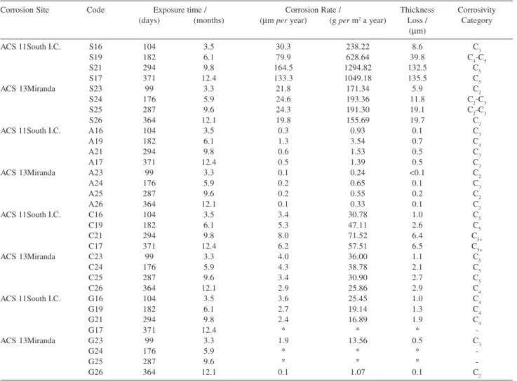
In Tables 8 and 9 the corrosion rates and the thickness loss for carbon steel, aluminum, copper and galvanized steel are presented, as well the classification in categories of corrosivity.
Based on the results and on the visual inspection, the corrosivity degree in the natural weathering sites could be classified in a decreasing order, according to the corrosivity criterion.
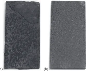
Carbon steel
ACS 11>> ACS 1> ACS 2> ACS 13. On Figure 6 the MSs surfaces are presented. The samples were evaluated after a year of exposition to natural weathering, at ACS 11 and ACS 13. The corrosion rate at ACS 11 was higher than at ACS 13.
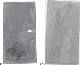
Aluminum
ACS 2> ACS 1> ACS 11> ACS 13. In Figure 7 the inspected MSs surfaces are shown after about a year of exposition to natural weathering, at the ACS 2 and 13. The corrosion rate was higher for ACS 2 than for ACS 13. The atmosphere of some areas in Sao Luis City is rich in chloride ions, which combined with moisture, produce hydrochloric acid (HCl). This acts as a strong oxidizing
Table 8. Results of the MSs exposed at ACSs 1 and 2
Corrosion Site Code Exposure Corrosion Rate / Thickness Corrosivity
time / (days) (µm per year) (g m-2per year) Loss / (µm) Category
ACS 1North I.C. S3 151 35.6 280.36 14.8 C3
S1 390 29.5 232.40 31.6 C3
S2 719 22.7 178.35 44.7 C5
ACS 2 Renascença S4 152 22.6 177.62 9.4 C2
S5 477 15.0 118.25 19.7 C4
S6 720 15.6 122.67 30.8 C4
ACS 1North I.C. A2 151 4.7 12.70 1.9 C5
A3 390 1.1 3.08 1.2 C4
A1 719 2.4 6.61 4.8 C5
ACS 2 Renascença A10 477 1.3 3.51 1.7 C4
ACS 1North I.C. C1 151 7.6 68.28 3.2 C5
C2 390 6.1 54.50 6.5 C5
C3 719 4.6 40.87 9.0 C5
ACS 2 Renascença C5 391 5.3 47.17 5.6 C5
C4 720 4.4 39.85 8.8 C5
ACS 1North I.C. G13 390 Negligible Negligible Negligible C1
G14 719 1.0 7.09 1.9 C3
ACS 2 Renascença G15 391 1.9 13.68 2.0 C3
G16 720 0.3 2.51 0.7 C2
Table 9. Results of the MSs exposed at ACSs 11 and 13
Corrosion Site Code Exposure time / Corrosion Rate / Thickness Corrosivity
(days) (months) (µm per year) (g per m2 a year) Loss / Category (µm)
ACS 11South I.C. S16 104 3.5 30.3 238.22 8.6 C3
S19 182 6.1 79.9 628.64 39.8 C4-C5
S21 294 9.8 164.5 1294.82 132.5 C5
S17 371 12.4 133.3 1049.18 135.5 C5
ACS 13Miranda S23 99 3.3 21.8 171.34 5.9 C2
S24 176 5.9 24.6 193.36 11.8 C2-C3
S25 287 9.6 24.3 191.30 19.1 C2-C3
S26 364 12.1 19.8 155.69 19.7 C2
ACS 11South I.C. A16 104 3.5 0.3 0.93 0.1 C3
A19 182 6.1 1.3 3.54 0.7 C4
A21 294 9.8 0.6 1.53 0.5 C3
A17 371 12.4 0.5 1.39 0.5 C3
ACS 13Miranda A23 99 3.3 0.1 0.24 <0.1 C2
A24 176 5.9 0.2 0.65 0.1 C3
A25 287 9.6 0.2 0.55 0.2 C2
A26 364 12.1 0.1 0.33 0.1 C2
ACS 11South I.C. C16 104 3.5 3.4 30.78 1.0 C5
C19 182 6.1 5.3 47.11 2.6 C5
C21 294 9.8 8.0 71.52 6.4 C5+
C17 371 12.4 6.2 57.51 6.5 C5+
ACS 13Miranda C23 99 3.3 4.0 36.00 1.1 C5
C24 176 5.9 4.3 38.78 2.1 C5
C25 287 9.6 3.4 30.90 2.7 C5
C26 364 12.1 2.9 25.86 2.9 C4
ACS 11South I.C. G16 104 3.5 3.6 25.45 1.0 C4
G19 182 6.1 2.7 19.14 1.3 C4
G21 294 9.8 2.4 16.89 1.9 C4
G17 371 12.4 * * *
-ACS 13Miranda G23 99 3.3 1.9 13.56 0.5 C3
G24 176 5.9 * * *
-G25 287 9.6 * * *
-G26 364 12.1 0.1 1.07 0.1 C2
agent and dissolves the passivated aluminum oxide layer (alumina - Al2O3), characterizing the pitting corrosion attack, as it can be seen in Figure 8. The A1 MS aged 24 months showed pits up to 75 µm deep. B17 and B26 MSs, both aged 12 months and A10 MS aged 16 months, showed pits up to 25 µm deep.
Another way to identify the pitting attack in the MSs was calculating the number of pits per area. A1 MS presented around 137 pits/cm2; A10 MS presented 40 pits/
cm2; B17 MS presented 48 pits/cm2; and B26 MS
presented 33 pits/cm2.
Copper
ACS 1≅ACS 11>ACS 2>ACS 13. In Figure 9 the assessed MSs are shown after about a year of exposition to natural weathering, at ACSs 1 and 13. The corrosion rate was higher for ACS 1 than for ACS 13.
The copper MSs submitted to natural weathering presented higher corrosion rates than those for aluminum, characterizing the regions of the ACSs in Sao Luis city as C5 (very high) corrosivity degree for this material. A closer evaluation shows a wide pit attack, as it can be seen in details by OM in Figure 10.
Galvanized steel
ACS 2>ACS 11>ACS 13>ACS 1. In Figure 11 the assessed MSs are shown after a year of exposition to natural weathering, at ACSs 1 and 2. The corrosion rate was lower for ACS 1 than for ACS 2.
All the ACSs, regardless from the exposed material, presented a stabilization of the corrosion rate along the time, faster for aluminum followed by copper and carbon steel.
After a year of the exposition, the corrosive atmosphere of the Southern I. C. (ACS 11) led to a more aggressive
Figure 6. Carbon steel MSs after a year of exposition to natural weather-ing (a) ACS 11-A17 MS, higher aggressiveness; (b) ACS 13–A 26 MS, lower aggressiveness.
Figure 7. Aluminum MSs after a year of exposition to natural weather-ing, (a) ACS 2–A10 MS, higher corrosivity; (b) ACS 13–B26 MS, lower corrosivity.
attack to the carbon steel, followed by ACS 1 on the Northern I. C. (Itaqui region). This effect was attributed to the calculated τ fraction for the period of exposition from May 2002 to June 2003, being 34% for ACS 1 and 49% for ACS 11 in the period of May 2004 to May 2005. The calculated τ justifies the higher rate of corrosion for ACS 11, even considering the lower quantity of pollutants in the corrosion site.
The galvanized steel MSs from ACSs 11 and 13 did not present a good performance due to their low Zn thickness (± 30 µm), deposited by hot dip process. For ACSs 1 and 2 it was just the opposite, where galvanized steel with thickness of 100 µm presented a better result.
It was also observed that galvanized MSs with low thickness coating presented a white oxide on the surface, not possible to be extracted by the Standard.18 It was
observed a mass increase, that made impossible to calculate the corrosion rate.
Figure 9. Copper MSs after approximately a year of exposition to natu-ral weathering, (a) ACS 1–C2 MS, higher aggressiveness; (b) ACS 13–C26 MS, lower aggressiveness.
Figure 11. Galvanized steel MSs after approximately a year of exposition to natural weathering: (a) ACS 2–G15 MS, higher aggressiveness; and (b) ACS 1–G13 MS, lower aggressiveness.
Atmospheric corrosivity rate
Based on the monitoring averages of the atmospheric pollutants (chlorides and sulfates) in the most critical period – July to December, the ACSs classification was built according to the atmospheric corrosivity rate, as shown in Tables 10 and 11.
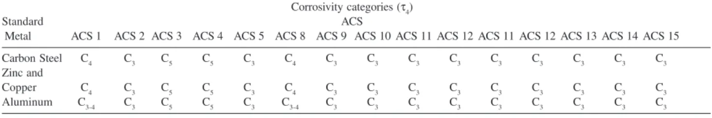
In Table 12, the atmospheric corrosion rates for the analyzed metals for each ACS are presented in corrosivity categories, based on the results of the pollutants and on the τ (Table 4 data was used to estimate the atmospheric corrosivity of these studied materials).
Table 13 rates the respective ACSs according to the type of corrosive environment and according to Liesegang
apud Kenny et al. criterion.12
ACSs 5, 14 and 15 were classified as rural environ-ments of low aggressiveness since they presented low chloride deposition rate (± 14.5 mg per m2 a day). ACS 3
region was the most corrosive in the atmospheric corrosivity category, presenting very high corrosivity, being followed by ACS 4.
ACS 1 and ACS 11 atmospheres were classified as very high category, presenting high quantities of dustfall. ACS 8 is also in the high corrosivity category and ACS 2 in the medium corrosivity one, showing an unexpected
Table 13. Corrosivity categories estimated in the atmosphere of the ACSs of São Luis City according to Liesegang apud Kenny et al.12 criterion
Corrosivity categories
Corrosive ACSs
Environment ACS 1 ACS 2 ACS 3 ACS 4 ACS 5 ACS 6 ACS 7 ACS 8 ACS 9 ACS 10 ACS 11 ACS 12 ACS 13 ACS 14 ACS 15
Rural
•
•
•
Marine
•
•
•
•
•
•
•
•
•
•
•
•
Note: ACSs 9, 10, 12 and 13 were considered marine environments for having a chloride deposition rate of about 30 mg Cl–per m2 a day in the dry period.
Table 12. Corrosivity categories of the ACS of São Luis City, estimated in the atmosphere
Corrosivity categories (τ4)
Standard ACS
Metal ACS 1 ACS 2 ACS 3 ACS 4 ACS 5 ACS 8 ACS 9 ACS 10 ACS 11 ACS 12 ACS 11 ACS 12 ACS 13 ACS 14 ACS 15
Carbon Steel C4 C3 C5 C5 C3 C4 C3 C3 C3 C3 C3 C3 C3 C3 C3
Zinc and
Copper C4 C3 C5 C5 C3 C4 C3 C3 C3 C3 C3 C3 C3 C3 C3
Aluminum C3-4 C3 C5 C5 C3 C3-4 C3 C3 C3 C3 C3 C3 C3 C3 C3
Note: C2,low corrosivity; C3, medium corrosivity; C4, high corrosivity and C5, very high corrosivity. Table 11. Classification of pollution by sulfur-containing substances represented by (SO2)
SO2 / (mg per m2 a day)
Corrosive ACSs
Environment ACS 1 ACS 2 ACS 3 ACS 4 ACS 5 ACS 6 ACS 7 ACS 8 ACS 9 ACS 10 ACS 11 ACS 12 ACS 13 ACS 14 ACS 15
P0
•
•
•
•
•
•
•
•
•
•
•
•
•
P1
•
•
P2 P3
Table 10. Classification of ASCs’ pollution by airborne salinity represent by chloride
Cl– / (mg per m2 a day)
Corrosive ACSs
Environment ACS 1 ACS 2 ACS 3 ACS 4 ACS 5 ACS 6 ACS 7 ACS 8 ACS 9 ACS 10 ACS 11 ACS 12 ACS 13 ACS 14 ACS 15
S0
•
S1
•
•
•
•
•
•
•
•
S2
•
•
•
•
Table 14. Aggressiveness categories estimate for each ACS
ACSs Aggressiveness Categories
ACS 1 – I.C. North-Itaqui Region High C4.5
ACS 2 – Renascença – mangroves Médium C3.5
ACS 3 – Praia do Meio – seashore Very high C5.0
ACS 4 – Panaquatira Seashore, strong winds Very high C5.0
ACS 5 – UEMA – College Campus Low C2.0
ACS 6 – Praia do Meio, 1000 m off the shore High C4.5
ACS 7 – Forquilha - Electric Energy Substation Medium / high C3.5
ACS 8 – Ribamar - Electric Energy Substation Medium C4.0
ACS 9 – Caolho - 1000 m off the shore Medium C3.0
ACS 10 – Urban center - 2000 m off the shore Medium C3.0
ACS 11 – I.C. – South Medium C3.0
ACS 12 – Santa Rita Low C2.0
ACS 13 – Miranda Low C2.0
ACS 14 – São Mateus Low C2.0
ACS 15 – Peritoró Low C2.0
low sulfur-dioxide deposition rate, along with ACS 7, ACS 9 and ACS 15.
Intense reddish darkening was observed in ACS 1 MSs due to an iron-ore deposit, that occurred on the metallic components and installations of the electricity transmission lines nearby.
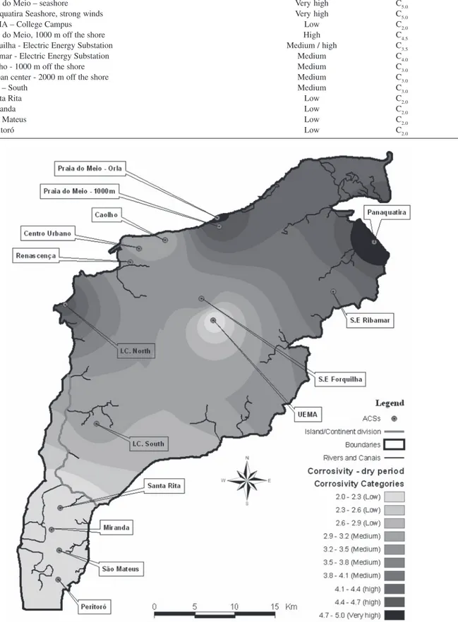
Atmospheric corrosivity map
The atmospheric corrosion map of Sao Luis City is represented in Figure 12. It was used the classification criteria based on the environmental data in the most critical period (dry season) and its effect on the corrosive resistance performance of the materials. It was taken the average values generated by a monthly monitoration of chlorides and sulfur-containing substances in each ACS during the dry period (between July and December). From these averages, it was estimated the atmospheric corrosivity for each ACS region, as a function of the wetness time (τ4), as presented in Table 14.
Conclusions
The atmospheric corrosive potential for Sao Luis City, determined by Brooks’ index, was 4.7. This classifies the atmosphere of the city as aggressive and with a moderate to high deteriorating rate.
During the measurement time, the region climate was driven by the equatorial and tropical air masses, which classified local atmosphere in two well defined seasons: the dry one (Jul-Dec) and the rainy one (Jan-Jun), according to Köppen’s methodology as Aw-tropical.5
Based on the climatic data, the presented condition during the study period of high RH% (superior to 70%) and the average temperatures of 30 ºC, resulted in a τ4. This is 50% of the annual fraction and favors the degradation process of the atmospheric metals.
In visual inspections at the distribution towers, it could be observed corrosion and erosion on the metallic components, mainly on the surfaces facing the North-East direction of the predominant winds.
Chloride deposition rate was more expressive than sulfur-containing substances represented by SO2, due to the predominance of a marine environment. It was observed that total sulfate deposition rate followed the chloride amount profile, which can be clearly evidenced at ACSs 3 and 4.
The highest dustfall rates were recorded at ACSs 1 and 11, both of them next to I.C., that are in agreement to the highest corrosion rates found in these sites.
The atmospheric conditions of the analyzed regions in Sao Luis City, in accordance with ISO 9223,7 led to a
classification for the corrosion on copper, as corrosivity C5, which is very high. For carbon steel the corrosivity was classified from high to very high for ACSs 1, 2 and 11. For ACS 13 it was classified as medium to low due to its low quantity of recorded chloride and sulfate amounts. During the study, the environmental aggressiveness for carbon steel and aluminum, given the influence of the contamination by pollutants, mainly chloride ions (Cl–),
and the climate conditions, resulted in high to very high atmospheres for both ACSs 1 and 2.
The galvanized MSs of ACSs 11 and 13, with a ± 30
µm zinc coating initial thickness, presented coating partial dissolution with a localized attack on the substrate, since the initial thickness was not enough to offer cathodic protection to carbon steel during the exposition period. On the other hand, ACSs 1 and 2 presented corrosivity C1 to C3 due to their initial coating thickness of about 100 µm.
The atmospheric corrosivity map for Sao Luis area showed that the more aggressive regions, with a C5 corrosive category in accordance with ISO 9223,7 were
ACSs 3 (Praia do Meio - on the seashore), and ACS 4 (Panaquatira). It is evident the great influence of the chloride ions deposition rate in this classification. It could be observed that in the region of Panaquatira, there should be carried out further evaluations with more ACSs. A better visualization of the local corrosivity could be defined, according to the shading chloride concentration gradient shown in the map. It is clear that the most central stations are under lower aggressive conditions due to the lower chloride deposition rates, which gradually decreases with the seashore distance, as seen in ACSs 7 and 9 to the North and in ACSs 11 to 15 to the South.
Acknowledgments
The authors would like to thank Companhia Energética do Maranhão – CEMAR (Maranhão Energy Company), Centrais Elétricas do Norte, ELETRONORTE (Northern Electricity Center), LACTEC, ANEEL and UFPR/PIPE for their technical and financial support, as well as the academic opportunity for developing this work.
References
1. Viana, R. O.; O Programa de Corrosão Atmosférica Desenvolvido pelo CENPES, Technical bulletin PETROBRAS, 1980, 23-1, p. 39.
3. Gentil, V.; Corrosão, 4th ed., LTC-Livros Técnicos e Científicos S.A.: Rio de Janeiro, 2003, p. 341.
4. Feliú, S.; Morcillo, M.; Corrosión y Protección de los Metales en la Atmósfera, Centro Nacional de Investigaciones Metalúrgicas, Ediciones Bellaterra S. A.: Madrid, 1982, p. 246. 5. Morcillo, M.; Almeida, E.; Rosales, B.; Uruchurtu, J.; Marrocos, M.; Corrosión y Protección de Metales en las Atmósferas de Iberoamerica: Programa CYTED, Gráficas Salué: Madrid, 1998, p. 816.
6. Roberge, P. R.; Klassen,R. D.; Haberecht, P. D.; Mat. Design
2002, 23, 321.
7. ISO 9223: Corrosion of Metal and Alloys - Classification of Corrosivity of Atmospheres, Genebra, 1992, p. 18.
8. ISO 9224: Corrosion of Metal and Alloys – Guiding Values for the Corrosivity Categories, Genebra, 1992, p. 5.
9. ISO 9225: Corrosion of Metal and Alloys - Corrosivity of Atmospheres - Methods of Measurement of Pollution, Genebra, 1992, p. 10.
10. ISO 9226: Corrosion of Metal and Alloys - Corrosivity of Atmospheres - Determination of Corrosion Rate of Standard Specimens for the Evaluation of Corrosivity, Genebra, 1992, p. 4.
11. ABNT NBR 14643: Corrosão Atmosférica – Classificação da Corrosividade de Atmosferas, Rio de Janeiro, 2001, p. 11. 12. Kenny, E. D.; Cruz, O. M.; Silva, J. M.; Sica, Y. C.; Ravaglio,
M.; Mendes, P. R.; Mendes J.C.; Desenvolvimento de Metodologia para Monitoramento do Grau de Poluição nos Alimentadores de 13,8 kV e 69 kV da Ilha de São Luís, Curitiba: LACTEC, Technical Report, 2004, p. 98.
13. Perry, R. H.; Chilton, C. H.; Manual de Engenharia Química, 5th ed., Guanabara Dois S.A.: Rio de Janeiro, 1980, ch. 3, p. 50.
14. ABNT NBR 6211: Determinação de Cloretos na Atmosfera pelo Método da Vela Úmida, Rio de Janeiro, 2001, p. 6. 15. ABNT NBR 6921: Sulfatação Total na Atmosfera –
Determinação da Taxa pelo Método da Vela de Dióxido de Chumbo, Rio de Janeiro, 1981, p. 7.
16. ASTM D 1739: Standard Test Method for Collection and Measurement of Dustfall (Settleable Particulate Matter), Philadelphia, 1994, p. 4.
17. ABNT NBR 6209: Materiais Metálicos Não Revestidos – Ensaio Não Acelerado de Corrosão Atmosférica, Rio de Janeiro, 1986, p. 5.
18. ABNT NBR 6210: Preparo, Limpeza e Avaliação da Taxa de Corrosão de Corpos de Prova em Ensaios de Corrosão Atmosférica, Rio de Janeiro, 1982, p. 16.
19. ASTM G 1-90: Preparing, Cleaning, and Evaluating Corrosion Test Specimens, 1990, p. 7.
20. Jeyaprabha, C.; Sathiyanarayanan, S.; Muralidharan, S.; Venkatachari G.; J. Braz. Chem. Soc. 2006, 17, 61.
21. http://www.cptec.inpe.br, accessed in September 2005. 22. Camargo Libos, M. I. P. de; PhD Thesis, Universidade Federal
do Rio de Janeiro, Brazil, 2002.
23. Morcillo, M.; Chico, B.; Mariaca, L.; Otero, E.; Corros. Sci.
2000, 42, 91.