A STOCHASTIC COLORED PETRI NET MODEL TO ALLOCATE
EQUIPMENTS FOR EARTH MOVING OPERATIONS
SUBMITED: November 2007 REVISED: June 2008
PUBLISHED: September 2008 EDITOR: P. Katranuschkov
Bruno de Athayde Prata, M.Sc.
Program in Logistics and Operations Research, Federal University of Ceará, Fortaleza, Brazil [email protected]
Ernesto Ferreira Nobre Júnior, Professor Dr,
Department of Transportation Engineering, Federal University of Ceará, Fortaleza, Brazil [email protected]
Giovanni Cordeiro Barroso, Professor Dr,
Department of Physics, Federal University of Ceará, Fortaleza, Brazil [email protected]
SUMMARY: Earth moving operations can be represented as Discrete Events Systems (DES), which propitiates
qualitative and quantitative analysis. In this paper we propose a model using Stochastic Colored Petri Nets to represent the operational dynamics of earth moving work. For this purpose, a graphic and analytic model that represents the earth moving activities was idealized. Data were collected concerning a real case, followed by several simulations aiming at the economic assessment of the identified operational scenarios. As a conclusion of the study, it can be stated that Petri nets models provide an important instrument for decision makers when managing earth moving planning and execution.
KEYWORDS: Earth Moving Works, Simulation, Decision Making, Colored Petri Nets.
1.
INTRODUCTION
Earth moving refers to all the operations involving the cut, loading, haulage, unloading, grading, humidifying and compaction of materials in a civil engineering building, aiming to adequately shape the natural field to the specifications of the project.
According to Lima and Nobre Júnior (2004), because earth moving and paving services deal with a big number of heavy equipments and move thousands of tons of material, they require special attention from the builders and the employer organizations. Therefore, it is necessary that the movement of material between borrow pits and disposal sites be done in a rational way in order to achieve reduction in the cost of buildings.
In an earth moving process, contractors tend to use the equipment available instead of allocating the ideal num-ber of machines. In these situations, given the material to be used, its characteristics, information about the trans-portation roads and the modalities of haulage, a simulation model can determine the production and the time expected to the accomplishment of a certain activity by a plant team (Jayawardane and Price, 1994a).
The objective of the work reported in this paper was to create a model based on stochastic colored Petri nets that is capable of providing adequate understanding of the operational dynamics involving teams of loader and truck, which are employed in earth moving processes, as well as enabling the simulation of auxiliary operational scena-rios involved in construction planning.
2.
EARTH MOVING: BASIC CONCEPTS
2.1
Definition of an earth moving system
The focus of discussion in this section is the rational allocation of equipments to the activities of cut, haulage and unloading. According to Ricardo and Catalani (1990), the equipments used to this purpose can be classified in:
• Excavation and haulage units; • Excavation and loading units; • Haulage units.
Excavation and haulage units are the ones which excavate load and haulage materials of medium consistency at middle distances. Excavation and loading units are the ones which excavate the ground and load other equip-ment, i.e. the haulage unit, in a way that the complete cycle of earth moving, including the four basic operations mentioned above, can be executed by two distinct machines.
Usually, for the accomplishment of such operations, the following teams are employed: (i) excavator – truck; (ii) pusher – scraper; and (iii) loader – truck.
Excavators are extremely heavy-duty equipments of high productivity and elevated operational cost, dedicated to the operations of cut and loading. Their utilization is justifiable when the quantity of material to be removed is considerable or when the time required to this removal is little.
Scraper is an equipment capable of doing four of the basic earth moving operations: excavation, loading, haulage and unloading. To overcome the friction originated from the operation of cut, scrapers are usually supported by tractors, named pushers. A tractor of the kind pusher has a special sharp which makes possible pushing the scra-per. A team pusher – scraper has an elevated productivity, recommended for middle haulage distances. In the construction of highways involving little volumes of material, the most usual team is loader – truck. Loaders are equipments of small loading capacity, low operational cost and high agility, utilized in cuts, on material loading. Trucks are destined to the material haulage and unloading, being adequate to big hauling distances.
2.2
Method of teams dimensioning
The traditional method of loader and truck teams dimensioning, as frequently used in Brazil (cf. Ricardo and Catalani 1990), aims to determine the quantity of haulage units to be used conjointly with a loader.
The efficiency or production of a loader is calculated by expression (1) C × ω × E × k
Q =
T (1)
where:
• Q: loader’s production (m3/h); • C: loader’s capacity (m3);
• ω: Shrinkage factor of the excavated material; • E: efficiency factor of the machine’s production; • k: bucket’s efficiency factor;
• T: loader’s cycle time (h).
The number of load operations or travels required to the loading of the truck is determined via the loader as follows:
q n =
C × k (2)
where:
• q: truck’s capacity (m3); • C: loader’s capacity (m3); • k: bucket’s efficiency factor.
Next, the time necessary for the loader to complete the haulage load unit is determined as:
tC = n × T (3)
where:
• tC: time for the loader to complete the load of the truck (h); • n: number of load operations;
• T: loader’s cycle time (h).
The complete cycle time of the haulage unit is calculated by the following equation: 1 1
tB = tB C + dm × [
va +
vb
] + tD + tM (4)
where:
• tB: truck’s cycle time (h); B
• tC: time for the loader to complete the load of the truck (h); • dm: haulage middle distance (km);
• va: speed of the loaded vehicle (km/h); • vb: speed of the loaded vehicle (km/h); • tD: unloading truck’s time (h);
• tM: truck’s maneuver time (h).
The number of trucks to be attended by a loader will be: tBB
N = tC
(5) where:
• N: number of trucks to be attended by a loader; • tB :truck’s cycle time (h);
• tC: time for the loader to complete the truck’s load (h).
Practically, it is being observed that it is not probable that N is an integer number. However, as the number of equipments to be allocated to the earth moving in a stretch of road must necessarily correspond to a discrete number, the use of the integer number immediately higher or lower is opted for.
In the case of adopting the lower integer number, there will be idleness of the loader and the trucks will govern the production. In the other case, there will be idleness of the trucks and the loader will govern the production. In prac-tice, it is usual that the loader governs the production because this provides more flexibility to the work’s dynamics. The current method of loader and truck teams dimensioning has some limitations that can be specified as follows:
• it permits the idleness in the operation of equipments;
• it does not consider variations at the cycle times of the operations of the machines due to uncer-tainties as it is based on a deterministic model;
• it does not permit the analyst comprehension of the operational dynamics of the dimensioned team, making the work planning difficult.
2.3
Modeling applied to earth moving problems
Simulations approaches permit a better comprehension of the modeled system. However, they do not always provide good solutions. Optimization approaches often lead to a better configuration of the modeled system. Next, the analysis of some propositions of earth moving modeling systems is reported, highlighting benefits and disadvantages of each of them.
Jayawardane and Price (1994a, 1994b) presented a new approach to the optimization of earth moving operations. They propose the utilization of linear and integer programming together with computational simulation, so that the total cost of the building would be minimized. The possibility of considering the new model, the operations of the equipments and the duration of construction was an innovative effort at the time.
Marzouk and Moselhi (2000) present an IT system that aims at optimizing the earth moving operations using an object-oriented simulation approach. The proposed system consists of a simulation module, an equipment data-base, an equipment cost application and a reporting module. It can aid the planning of earth moving operation in the bidding stage and in the scheduling of equipments.
Henderson et al. (2003) propose a model utilizing the meta-heuristic Simulated Annealing, which optimizes the way of the equipments in an earth moving process, reducing the total distance covered by the equipments. This model brings as a result a reduction in the operational costs related to fuel consumption, operation time and equipments maintenance. A criticism on the approach is that, although it provides satisfactory results, it does not permit a com-prehension of the modeled system or even provide scenarios idealization. The model under consideration is basical-ly normative.
Yang et al. (2003) present a model based on fuzzy logic aiming at simulating the cycle time of an excavation unit. The approach provides an adequate solution to the problem related to an accurate time cycle forecasting. However, from the viewpoint of practical model application, the mechanisms of the fuzzy theory hinder its applicability in the area of civil engineering due to the high complexity of the mathematical theory.
Lima (2003) proposes a mathematical model which relates geometrical and geotechnical data of highway works with material distribution, aiming at minimal execution cost. The approach searches to optimize not only the earth moving but also the paving services and considers mixes utilization and mills allocation. This is a condition not considered in any of the other analyzed models. However, it does not address the earth moving operation and pa-ving equipments.
Alkass et al. (2003) present a computer model, called FLSELECTOR, dedicated to the equipment fleets selection in earth moving operations. Based on Queuing Theory, the model determines the number of trucks and excava-tors to be allocated in a certain operational context, supporting decision making.
Bargstädt and Blickling (2005) propose an IT system which realizes earth moving teams, permitting that the user establishes scenarios in real time. The system has a graphical user interface which provides for visualization of the established scenarios.
Moselhi and Alshibani (2007) present a robust system for planning, tracking and control of earth moving opera-tions. It combines a module of spatial technologies, utilizing a Global Positioning System (GPS) and a Geogra-phic Information System (GIS), and a module based on a genetic algorithm (GA). The GPS was used for data collection in real time, GIS was employed to tabulate and analyze the collected data and the GA was applied in an optimization phase.
Finally, Prata et al. (2005, 2007) suggest the Petri nets as a method for loader and truck teams dimensioning via simulation. The modeling utilized by the authors permits better comprehension of the operational dynamics of an earth moving work and enables easy establishment of several operational scenarios.
3.
COLORED PETRI NETS
autono-mata”. At the end of the 60s and beginning of the 70s, researchers from MIT in the USA developed the founda-tions of the concept of the Petri nets as we know today.
According to Murata (1989), Petri nets are a type of bipartite, directed and weighted graph, which can capture the dynamics of a Discrete Event System. The Petri nets provide a compact representation of a system because they do not represent explicitly all the space of states from the modeled system.
An ordinary Petri net is a 4-tuple PN = (P, T , Pre post), formed by a finite set of places P of dimension n, a finite set of transitions T of dimension m, an input condition Pre: P x T → N, and an output condition Post: P x T → N. To each place an integer non-negative number denominated token is associated.
Models with time restrictions can be developed via Petri nets, as shown e.g. in (Berthomieu and Diaz, 1991). Manufacturing, transportation and telecommunication systems are some of the examples of application of that methodology.
A limitation of the ordinary Petri nets, also called place/transition Petri nets, is the fact that they demand a large quantity of places and transitions to represent complex systems (as most real systems are). As the net expands, the general view of the modeled system starts to get compromised, and the analysis of the modeled system be-comes difficult to do.
Real systems often present similar processes which occur in parallel or concurrently, and they differ from each other only by their inputs and outputs. In the colored Petri nets, the quantity of places, transitions and arcs is, generally, sensibly reduced via the addition of data to the structure of the net.
According to Jensen (1992), a more compact representation of a Petri net is obtained via the association of a data set (denominated token colors) to each token. The concept of color is analogous to the concept of type, common among the programming languages.
According to Jensen (1992), a colored Petri net is a 9-tuple:
CPN = (Γ,P,T,A,N,C,G,E,I) (6)
where:
• Γ is a finite, non empty set of types, denominated colors set; • P is a finite set of places of dimension n;
• T is a finite set of transitions of dimension m;
• A is a finite set of arcs so that P ∩ T = P ∩ A = T ∩ A = ∅; • N is a node function, defined from A by P × T ∪ T × P; • C is a color function, defined from P on Γ;
• G is a guard function, defined from T;
• E is a function of expression of arcs, defined from A; • I is an initiation function, defined from P.
The colors set determines the types, operations and functions which can be associated to the expressions utilized on the net (arc functions, guards, colors, etc.) The sets P, T, A and N have analogous significance to the vertexes and precedence functions sets defined for the ordinary Petri nets. Color functions map every place on the net, including them in a color set. Guard functions map all the transitions on the net, moderating the stream of tokens according to Boolean expressions. Arc functions map each arc on the net, associating them to a compatible ex-pression with the possible colors sets. Finally, initialization functions map the places on the net associating them to the existent multi-sets.
The data association to the token makes the model more compact, but, on the other hand, a price is paid: the complexity of the precedence functions.
p2 p1
x
x
(a)
p3
p1
p2
(b) x
x p
3
t1 t1
Statement of the variables is: Color X; Var x: X;
x x
1`1+ 1`2
2`2
1`1
1`2
X X
X X
X
X 1`2
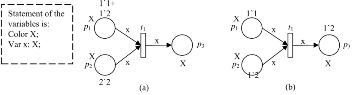
FIG 1: Example of firing of a transition in a colored Petri net.
The place p1 has a token of color 1 and a token of color 2 and the place p2 has two tokens of color 2. So, the fi-ring of t1 will remove a token of color 2 from each place, depositing a token of color 2 in p3.
A place can be seen as an indication of a state of the system (set of the current values of the parameters which define a certain system, in a certain instant). A place has the following attributes: (1) identification and (2) mar-king. Identification distinguishes a place from the others and the marking is equivalent to the number of tokens contained in a place. The tokens simply indicate that the conditions associated to the places are true.
Transitions can represent operations or actions accomplished by the system. They have the following attributes: identification and, for to the timed Petri nets, the time spent on firing. An arc which goes from a place to a tran-sition indicates, together with the tokens, the necessary conditions to an action to be accomplished.
A transition is considered capable to fire when the number of tokens contained in a place is greater than or equal to the weight of the precedence arcs. When this occurs, the transition t1 is enabled, being ready for firing. As we can see from the CPN presented in Figure 1, when the transition t1 fires, a token of color 2 is removed from the place p1, a token of color 2 is removed from the place p2 and a token of color 2 is put in the place p3.
According to Berthomieu and Diaz (1991), there are systems which have behavior based on explicit temporal parameters. Utilizing and amplifying the concept of the classical Petri nets, in other words, adding time charac-teristics to transitions provides the application of this technique to the modeling of systems related to various areas of knowledge.
In several practical applications of the Petri nets with time restrictions, determinism is a simplification. Even the random character of the timed Petri nets is not enough to represent, with likelihood, systems in which firing times are governed by density probability functions.
According to Cardoso and Valette (1997), a stochastic Petri net is obtained via the association of a function Λ, which is a function that associates, in each transition t ∈T, a transition firing ratio λ(t). So, the firing of each transition of a stochastic Petri net will be governed by an exponential distribution.
4.
CONCEPTION AND APLLICATION OF THE MODEL
4.1
Model Conception
Based on the theoretical foundations of the colored Petri nets described in Chapter 3, it was sought to represent the stages and the most meaningful events of a loader – truck operation by places and by transitions, respective-ly. In Figure 2, the CPN that models the system is shown.
FIG. 2: Colored Petri net, modeling a loader – truck team operation in an earth moving process.
TABLE 1: Legend of the places of the model presented in Figure 2.
Places
P1: loader next to cut P2: loader ready to load P3: quantity of cuts to be made P4: loaded loader
P5: loader ready to maneuver P6: loader ready to exceed P7: loader ready to unload
P8: quantities of cuts unloaded on the truck P9: truck hauling soil
P10: quantities of unloaded cuts P11: empty loader
P12: loader ready for new maneuver P13: empty truck
P14: truck returning
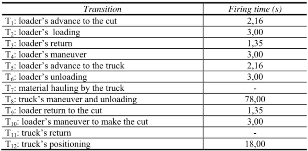
TABLE 2: Legend of the transitions of the model presented in Figure 2.
Transition Firing time (s)
T1: loader’s advance to the cut 2,16
T2: loader’s loading 3,00
T3: loader’s return 1,35
T4: loader’s maneuver 3,00
T5: loader’s advance to the truck 2,16
T6: loader’s unloading 3,00
T7: material hauling by the truck -
T8: truck’s maneuver and unloading 78,00
T9: loader return to the cut 1,35
T10: loader’s maneuver to make the cut 3,00
T11: truck’s return -
T12: truck’s positioning 18,00
The firing times of the transitions were calculated in accordance withthe method presented by Ricardo and Catalani (1990). As far as the firing times of the transitions T7 and T11 are concerned, they vary conform in each case because the trip time of a truck, as much going as returning, depends on the mean haul distance. Next, the firing times of transitions T7 and T11 are going to be defined for the studied case.
To apply the proposed model, data regarding the Brazilian junction project CE-187/311 (Viçosa do Ceará), fron-tier Ceará/Piauí (Padre Vieira), located in the State’s northwest region, were collected. In Figure 3, the Brückner diagram, obtained from the sheet of the accumulated volumes originating from the geometric projection of the highway, is illustrated.
Analyzing the graphic presented in Figure 3, it can be noticed that the extract at issue is predominantly from fill. For an application effect of the proposed model, it will be assumed that the material to be moved originated from a loan mine with 500 meters mean haul distance. Assuming that a truck can travel loaded with 30 km/h mean ve-locity and unloaded with 50 km/h mean veve-locity, the firing times of transitions T7 and T11 are going to be 60 s and 36 s, respectively.
The considered truck and loader capacities are respectively 10m3 and 2m3. For the purpose of carrying out a sen-sitivity analysis of the model, simulations have to be accomplished to dimension the machines’ team requested to accomplish the earth moving operation of the passages between piles 40 and 45, with volume of the fill in this passage equal to 8963,79 m3. Assuming as 1,4 the ratio between the specific weight of the material in the fill and in the cut, a cut volume corresponding to 12549,30m3 is requested, and, consequently, 6275 loader load
operations must be performed.
-120000 -100000 -80000 -60000 -40000 -20000 0 20000
0 20 40 60 80 100 120 140
Accumulated volumes (m3)
Marks (20m)
4.2
Background of the simulation’s modeling
The model was implemented and simulated utilizing the software CPNTools, a public domain program developed by Aarhus University, dedicated to modeling, simulation and analysis of Colored Petri Nets. This software posses-ses an interface which allows easy handling by the user, facilitating the specification of scenarios. Following, in Table 3, the results obtained in the simulations are presented.
The system in question has many uncertainties. Therefore, it was decided to accomplish a stochastic modeling of itself. As field data to the adjustment of probability density functions to the model’s transitions were not provi-ded, the premise that the operational times of the chain were governed by exponential distribution was adopted. This agreement was based on the following considerations:
• Exponential distribution is a continuous probability density function, currently used in the repre-sentation of service processes and of operations in the simulation studies’ processes;
• It is function of just one parameter, the firing time of the transitions. As times were not adhered, to estimate other parameters, and not only the mean time, would have had little practical value; • According to Bause and Kritzinger (2002), the reachability graph of a colored Petri net is
isomor-phic to a Markov Chain. Consequently, it is possible to accept that transitions among states are governed by an exponential distribution, in view of its character without memory.
Thus, in the computational model implemented in the software CPNTools, the firing times illustrated in Table 2 were considered as mean times governed by an exponential distribution.
The exponential distribution has a parameter, denominated λ, which represents the occurrence tax of a certain event. Such distribution has the following probability density function: (x) = e-λx
, for x
≥ 0, and f(x) = 0 otherwise. The exponential has a mean equal to 1/λ and variance equal to 1/λ2. For more details about the abovementioned distribution, see e.g. Evans et al. (1993).As the model is probabilistic, every time a simulation is made it will tend to offer distinct results in terms of cycle time. After computational experiments, it was decided to turn the model 10 times in order to obtain a value of mean cycle time that can be a good estimator of the system operation time.
The decision of considering 10 replications of the model can be explained as follows. For all studied scenarios, the variation coefficient (which is a statistic measure obtained by the division of the standard deviation by the mean) after 10 replications is small (between 0,27% and 1,72%). Therefore, the mean cycle time considering 10 replications can represent appropriately the operational timing of the system.
The simulation works in the following way: according to the concept of temporal Petri nets, presented in Bertho-mieu and Diaz (1991), the duration of the event after the firing of each transition can be related to it; hence, in the case of the model in focus, the time of each event will be exponentially distributed, with determined means as shown in section 4.1 above.
The CPNTools permit to associate to each token the time during the simulation. Thus, the cycle time will consist of the time accumulated, corresponding to the firing of the model transitions.
4.3
Computational experiments
In this section, a discussion of the Table 3, which summarizes the scenarios and the results of the accomplished computational experiments, is done. Columns 2 and 3 indicate the quantity of equipment used in each one of the scenarios and, in column 4, the cost of timetable operation of the allocated machines. The data inherent to the costs were obtained next to the Infrastructure Secretary of the State of Ceará. The fifth column corresponds to the cycle times’ average, in hours, obtained by CPNTools in ten simulated scenarios and, finally, the sixth co-lumn regards the operation cost of each one of the scenarios, obtained by the product of the forth and the fifth columns.
TABLE 3: Summary of the scenarios of earth moving.
Scenario Number of
loaders Number of trucks
Unitary cost (R$/h)
Mean cycle time(h)
Scenario cost (R$)
1 1 1 205,32 94,60 19424,20
2 1 2 269,99 50,48 13628,21
3 1 3 334,66 37,60 12584,06
4 1 4 399,33 33,91 13542,23
5 1 5 464,00 33,24 15421,22
6 1 6 528,66 33,15 17524,49
7 1 7 593,33 33,20 19696,14
8 1 8 658,00 33,21 21853,96
9 2 1 345,98 79,44 27484,53
10 2 2 410,65 40,70 16714,67
11 2 3 475,32 28,03 13322,10
12 2 4 539,98 21,91 11831,49
13 2 5 604,65 18,89 11419,01
14 2 6 669,32 17,32 11591,22
15 2 7 733,99 16,77 12305,33
16 2 8 798,66 16,63 13280,78
17 3 1 486,63 74,80 36402,40
18 3 2 551,30 37,68 20773,75
19 3 3 615,97 25,48 15695,10
20 3 4 680,64 19,38 13188,19
21 3 5 745,31 16,11 12008,91
22 3 6 809,98 13,90 11255,52
23 3 7 874,64 12,44 10880,48
24 3 8 939,31 11,69 10983,90
25 4 1 627,29 72,29 45345,95
26 4 2 691,96 36,17 25025,71
27 4 3 756,63 24,45 18501,51
28 4 4 821,29 18,50 15197,15
29 4 5 885,96 15,18 13453,31
30 4 6 950,63 12,76 12130,81
31 4 7 1015,30 11,17 11342,76
32 4 8 1079,97 10,11 10923,70
In Figure 4 the behavior of the cycle time variable for the simulated scenarios is presented. On the graph, the dependent variable corresponds to the operation time, while the independent variable concerns the number of trucks used in each scenario. On the graph there are four curves, one for each quantity of used loaders. Thus, it is possible to analyze the behavior of the loaders/trucks ratio and its influence on the cycle time variable. Concerning the numbers of loaders, it can be noticed that the cycle times in the scenarios employing just one loader are really higher than those which utilize 2, 3 or 4 loaders. Still analyzing the cycle time curve for one loader, it is possible to highlight that there is not a significant reduction in the cycle time for a loaders/trucks ratio less than 1/4.
For the curve inherent to the scenarios which employ 2 loaders, it can be underlined that the cycle time lessens in proportion to the scenarios with just one loader and that there is a convergence of the time cycle for a quantity of trucks greater than or equal to 7.
The scenario with lowest cycle time can be desirable when construction needs to be concluded with urgency, once that there would be some emergency character of the undertaking or some external time limit to be taken into account. However, the scenario with the lowest cycle time is not always the most desirable under economic viewpoint. Therefore, the simulations must point to the scenario whose operational cost is as low as possible.
0,00 10,00 20,00 30,00 40,00 50,00 60,00 70,00 80,00 90,00 100,00
0 1 2 3 4 5 6 7 8
1 loader
2 loaders
3 loaders
4 loaders
Cycle time (h)
Number of trucks
FIG. 4: Behavior of the cycle time variable for the simulated scenarios.
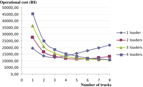
In Figure 5 the variable operational cost’s behavior for the simulated scenarios is presented. On this graph, the dependent variable corresponds to the cost of the scenario, while the independent variable is related to the num-ber of trucks employed in each scenario. Analogous to the graph on Figure 4, in Figure 5 there are four curves, one for each quantity of utilized loaders. In this way, the behavior of the ratio loaders/trucks and its influence on the cost of the operation variable can be analyzed.
0,00 5000,00 10000,00 15000,00 20000,00 25000,00 30000,00 35000,00 40000,00 45000,00 50000,00
0 1 2 3 4 5 6 7 8
1 loader
2 loaders
3 loaders
4 loaders
Operational cost (R$)
Number of trucks
FIG. 5: Behavior of the operational cost variable for the simulated scenarios.
The scenarios with 2 loaders are less expensive that those which utilize only one loader, but are less efficient than the ones employing 3 or 4 loaders. This tendency showed itself evident in the analysis of Figure 4. The scenarios with 3 or 4 loaders behave in a similar way for a number of trucks between 3 and 8. The scenario that represented the lowest operation cost was with the ratio loaders / trucks equal to 3/7, but the difference be-tween this value and the scenarios with the ratios 3/8, 4/7 and 4/8 is less than 4%.
4.4
Evaluation
For an evaluation effect of the benefits of the proposed approach, it is necessary to compare the results presented by the model with the current practice in the field of highway engineering, according to the discussion in section 2.2 above.
The calculation of the loader production determined according to equation (1) was 396 m3/h. It was based on the following parameters: C = 2m3; ω = 1,4; E = 0,83, k = 0,9 e T = 19s. The values of C and ω consist in premises adopted by the model. The values E and k are mean values put in practice, accrued of the authors’ experience, and the value T corresponds to the sum of the firing times of transitions T1, T2, T3, T4, T5, T6, T9 and T10. Applying equation (2), a value of six trips required for a truck loading is obtained. The loader’s cycle time was 0,192 h according to the equation (3). The truck’s time cycle was calculated based on the following values: tc = 0,192h; dm = 0,5km; va = 30km/h; vb = 50km/h e tD + tM = 78s. The value tc was obtained via equation (3), va and vb are input data of the problem, and the value 78s corresponds to the firing time of transition T8. Finally, by using equation (5), a team composed by a loader and eight trucks was obtained. It is relevant to acc-entuate that this operational alternative was simulated in the scenario 8 in Table 3. A comparison between the percentage deviation of the operational cost of all simulated scenarios and the operational cost of scenario 8 is illustrated in Figure 6 below.
Deviation (%)
Number of trucks
FIG. 6: Percentage deviation between the operational costs of the simulated scenarios and the operational cost obtained via the traditional method (scenario 8).
Analyzing the ratio loaders/trucks with regard to the difference between the scenarios costs and the cost ob-tained through the traditional method, the following observations can be underlined. When the number of trucks is small, it is not efficient to allocate a larger number of loaders. According to Figure 6, it is noticeable that the four scenarios that presented superior costs to the scenario corresponding to the traditional method have ratios equal to 1/2, 1/3, 1/4 and 2/4.
The benefit of employing a greater number of loaders increases when the number of trucks is greater than or equal to 6. The scenarios with ratios loaders/trucks equal to 2/5, 2/6, 3/7, 3/8, 4/7 and 4/8 incur in percent de-viation higher or equal to 47%, in proportion to the scenario 8, correspondent to the traditional method. The scenarios with ratios loaders/trucks equal to 1/3, 2/4, 3/5 and 4/6 have percent deviations with regard to scenario 8 in an interval of 42.4% to 45%, thus showing themselves as quite efficient. It has to be underlined that these scenarios also demonstrate an interesting behavior: from the scenario with one loader and three trucks on-wards, increasing the number of loaders in a unit, if the difference between the number of trucks and the number of loaders is maintained equal to 2, the efficiency of the scenarios tends to be similar.
5.
CONCLUSIONS
This paper presented the modeling of equipments operation in an earth moving process as a Discrete Events System (DES) and proposed the stochastic colored Petri nets method for modeling and analysis of the system. The relevance and originality of the proposed model is in first place in the application of colored Petri nets in an earth moving system which is not only innovation but also a great practical utility for the realization of opera-tional scenarios in earth moving operations.
As advantages of the proposed model, the following can be emphasized:
1) Propitiating a better comprehension of the operational dynamics of the modeled system, compared to the traditional method employed in Brazil;
2) Enabling the simulation of several operational scenarios at once to support decision making in the construction management;
3) The easy practical application.
The results of the simulations showed that more than 80% of the solutions created by the model based on colored Petri nets are better than the result of the traditional method employed in Brazil, which does not effectuate an efficient search in the variety of possible solutions. The use of simulation, albeit not guaranteeing achievement of an optimal solution, assesses a wider variety of possibilities and points to a convergence for the solution cost. It is also important to highlight that the proposed model can be utilized not only for conceiving scenarios with low costs, but also to conceive scenarios that complete goals concerning the accomplishment of timelines in a certain project. For instance, if delays occur in the project and the initial timeline for work completion can not be altered, the abovementioned model can be used to determine the necessary team for completion of the project in the required time.
With regard to the applicability of the proposed model, the following comments can be made. Although the Petri nets theory is based on a complex mathematical background, using an already established model is not a very hard task. The existence of software, as for example the CPNTools, makes the proposed model’s use in all soil moving processes completely plausible. By training the technical teams, autonomous simulations supporting decision making can be easily achieved.
As underlined in section 2.3, there are several approaches based on mathematic and computational modeling applied to earth moving problems. The main advantages obtained by the use of colored Petri nets in relation to these approaches are as follows:
1) The model is very flexible and can be readily customized for different earth moving operations; 2) The graphic model of the colored Petri net permits easy comprehension of the modeled system and
a good visualization of the simulation via animation;
This makes the Petri nets approach a powerful instrument for the implementation of the supervisory control in DES (Moody & Antsaklis, 1998, Iordache & Antsaklis, 1998).The supervisory control can coordinate the ope-ration of an earth moving work, thereby increasing the opeope-rational efficiency of the system.
However, the proposed model has also some limitations and simplifications that need to be mentioned: • Simulations do not point, necessarily, to the system’s optimal operation;
• The model considers that the equipments possess the same capacity and productivity.
As suggestions to the drilling down of the researched problems and improvement of the proposed model, the following can be recommended:
• Joint use of the proposed model with optimization algorithms in order to minimize the total cost of earth moving operation;
• Consideration of equipments with different productivities;
• Extension of the modeling to other basic activities of the earth moving and paving process; • Applying the supervisory control theory, based on Petri nets, aiming at a better performance of the
earth moving operations.
6.
REFERENCES
Alkass, S., El-Moslmani, K. and Al Hussein, M. 2003, A Computer Model for Selecting Equipment for Earth-moving Operations Using Queuing Theory, CIB REPORT, vol. 284, 1– 7.
Bargstädt, H. J. and Blickling, A. 2005, Implementation of Logic for Earthmoving Processes with a Game Deve-lopment Engine, 22nd. International Conference on Information Technology in Construction. Dresden, Germany.
Bause, F. and Kritzinger, P. S. 2002. Stochastic Petri Nets – An Introduction to the Theory, Vieweg, Lengerich. Berthomieu, B. and Diaz, M. 1991. Modeling and Verification of Time Dependent Systems Using Time Petri
Nets. IEEE Transactions on Software Enginering, vol. 17, 259 – 273.
Cardoso, J. and Valette, R. 1997. Redes de Petri, Editora UFSC, Florianópolis, Brasil.
Desrochers, A. A. and Al-Jaar, R. Y. 1995. Applications of Petri nets in manufacturing systems, IEEE Press. Evans, M., Hastings, N. and Peacock, B. 1993. Statistical distributions, John Wiley & Sons, New York. Henderson, D., Vaughan, E. D., Jacobson, S. H., Wakefield, R. R. and Sewell E. C. 2003. Solving the shortest
route cut and fill problem using simulated annealing, European Journal of Operational Research, vol. 145, 72-84.
Iordache, M. V. and Antsaklis, P. J. 2006. Supervisory control of concurrent systems: a Petri nets structural app-roach, Birkhäuser, Boston.
Jayawardane, A. K. W. and Price, A. D. F. 1994a. A New Approach for Optimizing Earth Moving Operations – Part I, Proceedings of Instn. Civil Engineers Transportation, 105, pp. 195-207.
Jayawardane, A. K. W. and Price, A. D. F. 1994b. A New Approach for Optimizing Earth Moving Operations – Part II, Proceedings of Instn. Civil Engineers Transportation, 105, pp. 249-258.
Jensen, K. 1992. Coloured Petri nets: basic concepts, analysis methods and practical use – Volume 1: basic con-cepts, Springler-Verlag.
Lima, R. X. 2003. Logística da Distribuição de Materiais em Pavimentação Rodoviária: uma Modelagem em Programação Matemática. Fortaleza. Dissertação (Mestrado) Programa de Engenharia de Transportes - PETRAN, Universidade Federal do Ceará, Brasil.
Lima, R.X. and Nobre Júnior, E. F. 2004. Logística Aplicada à Construção Rodoviária, V Recontre Internacio-nale de Recherche em Logistique - RIRL 2004, Fortaleza, Ceará, Brasil.
Moody, J. O. and Antsaklis, P. J. 1998. Supervisory control of discrete event systems using Petri nets, Kluwer Academic Publishers.
Moselhi, O. and Alshibani, A. 2007. Crew optimization in planning and control of earthmoving operation using spatial technologies, Journal of Information Technology in Construction - ITcon, v. 12, 121 – 137. Murata, T. 1989. Petri Nets: properties, analysis and applications, Proceedings of the IEEE, v. 77, 541-580. Prata, B. A., Nobre Júnior, E. F. and Barroso, G. C. 2005. Modelagem de sistemas de terraplenagem: uma
apli-cação das redes de Petri, XVI Iberian Latin American Congress on Computational Methods in Enginee-ring, Guarapari.
Prata, B. A., Nobre Júnior, E. F. and Barroso, G. C. 2007. Dimensionamento de equipes mecânicas em obras de terraplenagem usando redes de Petri coloridas, XXXIX Simpósio Brasileiro de Pesquisa Operacional, Fortaleza, Brasil.
Ricardo, H. S., Catalani, G. 1990. Manual Prático de Escavação – Terraplangem e Escavação de Rocha, Editora Pini, São Paulo, Brasil.