Lat. Am. j. solids struct. vol.11 número14

(1)

Abstract

A simple Trefftz-type finite element method (TFEM) is proposed for solving certain potential problems in orthotropic media. The “body force”, which is induced by internal sources or sinks, may produce domain integrals in the standard Trefftz finite element formulation. This will make the advantage “only-boundary inte-gration” of TFEM lose entirely. To overcome this difficulty, the dual reciprocity method (DRM) is employed to transfer the origi-nal problem into a homogeneous one. Then, a particular solution (PS) Trefftz-type finite element model is established based on the modified functional. Three benchmark examples are investigated by the proposed approach and compared with the analytical solu-tions.

Keywords

Orthotropic potential problem; “body force” term; Trefftz finite element method; modified functional; dual reciprocity method.

Trefftz-type FEM for solving orthotropic potential problems

1 INTRODUCTION

A wide range of problems in physics and engineering such as heat transfer, fluid flow motion, flow in porous media, shaft torsion, electrostatics and magnetostatics can finally come down to the solu-tion of potential problems. These problems in isotropic materials have been widely studied from both the analytical and numerical point of view. Due to the inherent mathematical difficulties, closed-form solutions exist for only a few simple cases. Many new high-performance materials exhib-it non-isotropic properties, which lead to more complicated equations governing their mechanical behaviors than well researched isotropic materials. Powerful methods to pursue numerical solutions are mainly based on the finite element method (FEM) and boundary element method (BEM). Among these methods, the Trefftz-type finite element method (TFEM), originally developed by Jirousek and Leon (1977), has recently received great attention. This finite element method with homogeneous solutions as internal interpolation functions was developed based on the framework of Trefftz method (Trefftz, 1926). In this method, two dependent assumed fields (intra-element filed and auxiliary frame field) are employed and the domain integrals in the variational functional can

K.Y. Wang a P.C. Li b D.Z. Wang c

College of Mechanical Engineering, Shanghai University of Engineering Science, Shanghai 201620, P. R. China

Corresponding author:

a _{k.y.wang@126.com} b _{iselee18@163.com}

c_{wdzh168@126.com}

(2)

Latin American Journal of Solids and Structures 11 (2014) 2537-2554

be directly converted to boundary integrals without any appreciable increase in computational ef-fort. Up to now, Trefftz-type elements have been successfully applied to numerous engineering prob-lems such as plate bending (Jirousek and Guex, 1986; Rezaiee-Pajand and Karkon, 2012), elasticity (Jirousek and Venkatesh, 1992; Choi et al., 2006), potential problems (Fu and Qin, 2011; Wang el al., 2012), piezoelectricity (Qin, 2003), elastoplasticity (Zieli_ński, 1988; Bussamra et al., 2001; Qin, 2005), poroelasticity (Moldovan, 2013), etc.

As highlighted by Jirousek and Venkatesh (1992); Qin (2000; 2008), the TFEM couples the advantages of FEM and BEM. Due to the fact that no domain integrals are involved in the for-mulation of TFEM, the Trefftz-type elements are less sensitive to mesh distortion in practical applications. This feature has been investigated by Jirousek and Wroblewski (1995); Jirousek and Qin (1996); Choi et al. (2006); Cen et al. (2011); Wang et al. (2012) using different 4-node quad-rilateral elements. On the other hand, the employment of two independent fields also makes the TFEM easier to generate arbitrary polygonal or polyhedral elements with or without inclusions, which are accurate, efficient and natural for micromechanical modeling of heterogeneous materials (Dong and Atluri, 2012a,b,c). And the special-purpose elements of TFEM, which may achieve a level of popularity unequalled nowadays, can efficiently capture the stress concentration (or high gradients) without mesh refinement. These special elements with embedded complexities, which use complete general solutions in the domain, can greatly reduce the computational burden and preprocessing effort. Among the researchers who made contributions to special elements, the work of Piltner (1985); Jirousek and Venkatesh (1992); Leconte et al. (2010); Wang and Qin (2011; 2012a; 2012b) should be mentioned. Besides, there is also another kind of special element which can capture the singularity at crack-tip (Freitas and Ji, 1996; Kaczmarczyk and Pearce, 2009). Zhao and Zhao (2011) recently proposed a hybrid finite element model for anisotropic poten-tial problems. In their model, the fundamental solutions are used as trial functions for element field. Wang et al. (2012) developed a novel Trefftz finite element model, whose intra-element interpolation functions can reflect varying properties, for simulating heat conduction in nonlinear functionally graded materials (FGMs). Wang et al. (2012) recently focused their atten-tion on the orthotropic potential problems. The original problem is mapped into an equivalent isotropic one by coordinate transformation so that Trefftz functions are readily obtained from Laplace equation. In the meantime, the original boundary conditions must also be transformed before their imposition on the new domain. For a potential problem with “body force”, a domain integral will also be required. This may cause one of the key features of TFEM, namely its “only-boundary integration” formulation, to lose entirely. To smooth out this difficulty, a dual reciproc-ity method (DRM) developed by Wrobel et al. (1986); Nardini and Brebbia (1987) has usually been used for handling the potential problems with “body force” in isotropic bodies by Cao et al. (2012); Kita (2005); Wang et al. (2012); Balakrishnan and Ramachandran (1999). However, rela-tively few contributions applying TFEM to orthotropic potential problems with “body force” can be found in the literature.

(3)

(RBFs) for which particular solutions can be easily determined. To alleviate the inconvenience as addressed in the work (Wang et al., 2013), an alternative modified functional has been established for homogeneous orthotropic problems so that the solution process can be conducted in the origi-nal domain. As a benchmark, three examples are numerically investigated and a fair agreement is found in comparison with analytical solutions.

2 BASIC EQUATIONS AND DRM

2.1 Basic equations

Let us consider a 2D well-posed, orthotropic potential problem

(

)

2 2

1 ₂ 2 ₂ ,

u u

k k f X Y

X Y

¶ ¶

+ =

¶ ¶ in W (1)

subjected to the Dirichlet boundary condition

(

)

(

)

u X,Y =u X,Y on G_u (2)

and the Neumann boundary condition

(

)

1 1 2 2

(

)

u u u

q X,Y k n k n q X,Y

n X Y

¶ ¶ ¶

= = + =

¶ ¶ ¶ on Gq (3)

where u and q are the potential and its derivative in normal direction, f is the term of “body force” induced by internal sources or sinks, k1 and k2 are the horizontal and vertical material coefficients, respectively, and they are assumed to be parallel to the major axes of anisotropy, n1 and n₂ are direction cosines of the outward normal to the boundary, G denotes a bounded do-main in _Â2_{space with boundary}_G_,

u q

G = G È G . The (·) quantities indicate prescribed bound-ary values.

For the sake of clarity, Eq. (3) is rewritten in the matrix form as

(

)

u u T

(

)

q X,Y q X,Y

X Y

é¶ ¶ ù

ê ú

= _ê _ú =

¶ ¶

ë û

A withA= êé_ëk n_{1 1} k n_{2 2}ù_ú_û (4)

2.2 Methodology of DRM

In order to solve the potential problems with “body force” by boundary-type methods, it is neces-sary to eliminate the right-hand side in Eq. (1). This can be done by decomposing the solution to Eq. (1) into two parts, namely a particular solution up and a homogeneous solution uh, such that

p h

(4)

in which

(

)

2 2

1 ₂ 2 ₂

p p

u u

k k f X,Y

X Y

¶ ¶

+ =

¶ ¶ (6)

and

2 2

1 ₂h 2 h₂ 0

u u

k k

X Y

¶ ¶

+ =

¶ ¶ (7)

together with the modified boundary conditions

-h p

u =u u on G_u (8)

h p

q = -q q on Gq (9)

To obtain the particular solution up and homogeneous solution uh, we can rewrite the

differ-ential operator in Eq. (1) as follows (Wang et al., 2012)

2 2 2 2

1 ₂ 2 ₂ ₂ ₂

1

ˆ ˆ

k k r

r r r

X Y X Y

æ ö

¶ ¶ ¶ ¶ ¶ _ç _{¶ ÷}

+ = + = ç_ç ÷_÷_÷

è ø

¶ ¶

¶ ¶ ¶ ¶ (10)

where

1

ˆ X

X k

= ,

2

ˆ Y

Y k

= , 2 2

1 2

X Y

r

k k

= + (11)

By virtue of Eqs. (6) and (10) the particular solution u_p can be straightforwardly expressed as

(

)

d d 2 1

r r

p _r _r

u =

ò ò

f X,Y r r (12)

where r1 and r2 are arbitrary reference values. It is noted that up dose not necessarily satisfy

the boundary conditions (2) and (3) and is not unique. Besides, the exact expression for u_p can be explicitly obtained using Eq. (12) if f X,Y

(

)

is constant or in a simple form. However, it is often intractable or even impossible to get the analytical derivation of up

(

X,Y

)

when f X,Y

(

)

is a general function. Thus, the approximate particular solution becomes necessary. To deter-mine the particular solution u_p

(

X,Y

)

, the right-hand side term f X,Y

(

)

in Eq. (1) is usually approximated in the manner

(

)

(

)

1

L

k k

k

f X, Y a j X, Y

=

»

å

(13)

(5)

coefficients, and j_k

(

X, Y

)

denote the basis functions in which the RBFs are selected in this pa-per. Now, the problem of finding a particular solution is reduced to

(

)

(

)

₍

₎

2 2

1 ₂ 2 ₂

k k

k

X,Y X,Y

k k X,Y

X Y

F F

j

¶ ¶

+ =

¶ ¶ (14)

where F_k

(

X,Y

)

is a closed-form particular solution corresponding to j_k

(

X,Y

)

. Subsequently, the approaximate particular solution up

(

X,Y

)

can be expressed as follows (Qin and Wang, 2008)

(

)

(

)

1

L

p k k

k

u X,Y a F X,Y

=

å

(15)

It is always difficult in finding F_k

(

X,Y

)

by solving Eq. (15) directly. Hence, we can rewrite Eq. (14) in the following form

(

)

(

)

(

)

2 1 k

k k

X,Y

X,Y F X,Y

F r j

r r r

æ _¶ ö_÷

ç

¶ _ç _÷_÷

 = ç_ç _÷_÷=

¶ ç_è ¶ ÷_ø (16)

wherer =

(

X-Xk

)

2 k₁ +

(

Y -Yk

)

2 k₂. Performing integration twice analytically for Eq. (16),

the corresponding F_k

(

X, Y

)

can be readily determined. Here, the power spline-type RBFs in Â2 space such that

(

)

3

k X,Y

j = r are chosen. Therefore, we arrive at

(

)

₂₅5

k X, Y

r

F = (17)

Consequently,

(

)

3 -5 k k X X X F r ¶ =

¶ (18)

(

)

3 5 k k Y Y Y F r ¶ =

-¶ (19)

Once F_k

(

X, Y

)

are obtained according to Eq. (16), we can solve Eq. (13) for determination of the unknown coefficients ak by means of the singular value decomposition (SVD). Then, the

particular solution u_p

(

X,Y

)

can be evaluated at any field point from Eq. (15). The corresponding particular heat flux q_p

(

X,Y

)

may be readily expressed as

(

)

(

)

1 L k p p k k X,Y u q X,Y n n F a = ¶ ¶ = =

(6)

3 TREFFTZ-TYPE FINITE ELEMENT FORMULATION

3.1 Assumed fields

To solve the orthotropic potential problem governed by Eqs. (1)-(3) using TFEM approach, the solution domain W has to be divided into a number of elements as done in the conventional FEM. For each element e_{occupied by a sub-domain}

e

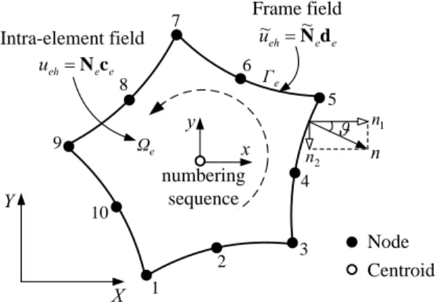
W , two independent fields (Jirousek and Qin, 1996; Qin and Wang, 2008; Wang et al., 2012), i.e. intra-element potential field and frame potential field, are assumed as shown in Figure 1.

(i) Intra-element potential field

( )

m

( )

eh ej ej e e

j =1

u x,y =

å

N c =N x,y c in W_e (21)

(ii) Frame potential field

( )

eh e e

u x,y =N x,y d on G_e (22)

where Ne is a vector of interior trial functions in which a finite terms only of homogeneous

solu-tions to Eq. (1) are retained and are called Trefftz funcsolu-tions, c_e is of the unknown parameters

ej

c , N_e is of the conventional shape functions and d_e is of nodal degrees of freedom (DOF) of the element. The symbol “~” allows the two fields to be distinguished and

(

x,y

)

is the local Cartesian coordinate system. The proper number m of truncated set of homogeneous solutionsN_ej is chosen in such a way that (Qin and Wang, 2008)

1

d

m ³m - (23)

to avoid spurious zero-energy modes. Here, m_d denotes the number of nodal DOF of the element. It should be noted that Eq. (23) is only a necessary but not a sufficient condition. In practice, more Trefftz functions are usually required to guarantee the resulting element stiffness matrix with full rank and to stabilize the performance of the element (Jirousek and Venkatesh, 1992).

1

2 3

4 5 6

7

8

9

10

e e eh

~ u~ Nd

Frame field

e e eh u Nc

Intra-element field

numbering sequence

x

y _ n1

2

n n

X Y

e

Ω

e

Γ

Node Centroid

(7)

In the framework of TFEM, the homogeneous solution uh is approximated as a superposition

of Trefftz functions L_k that exactly satisfies the governing differential equation (7). For the Laplace equation over a 2D bounded domain, a set of homogeneous solutions to Eq. (1) is given by (Wang et al., 2012)

( ) ( )

{

Re k , Im k kcos , ksin

}

k z z r k rq kq

L = =

(

k =1 2, ,,¥

)

(24)

where 1 2 k y tan k x

q = (25)

Truncating m_{terms of homogeneous solutions for Eq. (24), the vector of Trefftz functions}

e N

can be explicitly written as

( )

{

}

2

1 2 ... 1 cos , sin ₁ m

k k

e = é_ëê e e e m- emúù_û= r k rq kq _k₌

N N N N N (26)

It can be observed from Eq. (26) that Ne0 =1, which represents the rigid-body motion mode, is excluded from Ne in generating the sequence Nej. As a result, m should always be an even

number (Qin and Wang, 2008).

From Eq. (21), the corresponding outward normal derivative of u_e may be readily deduced as

( )

1

m

eh ej ej e e e e

j

q x,y Q c x,y x,y

=

å

=AT c =Q c (27)

where

T

e e

e

x y

é_¶ _¶ ù

ê ú

= ê _¶ _¶ ú

ë û

N N

T (28)

with

(

)

(

)

{

1 1

}

2

1 1

1

cos 1 sin 1

m

e k k

k

kr k , kr k

x k q q

- -= ¶ = - -¶ N (29)

(

)

(

)

{

1 1

}

2

1 2

1

sin 1 cos 1

m

e k k

k

kr k , kr k

y k q q

- -= ¶ = - - -¶ N (30)

(8)

1 2 3

0 0 0 0 0 0 0

e = êéë N N N ùúû

   

N (31)

1 2 3 4 5 6 7 8 9 10

e = êéëu u u u u u u u u u ùúû

d (32)

where u_k

(

k =1, 2,,10

)

is the potential change at the k_{th node, and}

(

_{1, 2, 3}

)

i

N i= represents the conventional shape functions in terms of natural coordinates x Î -é_ê_ë 1, 1ù_ú_û

(

)

1 1

1 2

N = - x -x , 2

2 1

N = -x , ₃ 1

(

1

)

2

N = x +x (33)

3.2 The finite element stiffness equation

To establish the linkage between the two independent fields (21) and (22), a modified variational functional, which includes boundary integrations only, is constructed based on the work of Wang and Qin (2008):

(

)

1

d d d d

2 e eu eq eI

me _G q ueh eh _G q ueh eh _G qe qep qeh ueh _G q ueh eh

P =

_ò

G -

_ò

 G +

_ò

- -  G -

_ò

 G (34)

where G = G È G È Ge eu eq eI,G = G Ç Geu e u,G = G Ç Geq e q, andGeI is the inter-element boundary

between elements.

Further, Eq. (34) may be readily rewritten in a compact form

(

)

1

d d d

2 e e eq

me _G q ueh eh _G q ueh eh _G qe qep ueh

P =

_ò

G -

_ò

 G +

_ò

-  G (35)

Then, substitution of Eqs. (21), (22) and (27) into the functional (35) leads to

1 2

T T T

me e e e e e e e e

P = c H c -c G d +d p +terms without c_e and/or d_e (36)

where

(

)

d , d , d

e e e

T T T

e =

ò

_G e e G e =

ò

_G e e G e =

ò

_G e qe -qep G

H Q N G Q N p N (37)

To ensure good numerical conditioning of H_e and to prevent overflow or underflow in evaluat-ing the inverse of He, the introduction of a local non-dimensional coordinates system

(

x h,

)

is

usually suggested such that (Jirousek and Venkatesh, 1992; Qin and Wang, 2008)

(

)

(

)

l l 0 1 0 1 1 1 n

c c i c

i l

n

c c i c

i l

x a X X a X X a

n

y a Y Y a Y Y a

n x h = = æ _ö÷ ç _÷ ç

= = - =ç_ç - ÷_÷_÷

çè ø

æ _ö÷

ç _÷

ç

= = - =_ç_ç - ÷_÷

÷

çè ø

å

(9)

where Xo and Yo are global Cartesian coordinates of element centroid, nl is the number of

ele-ment nodes and a_cthe average distance between centroid and nodes of the element.

To enforce inter-element continuity on the common element boundary, the unknown vector c_e

should be expressed in terms of nodal DOF d_e. The stationary condition of the functional P_me

with respect to ce and de, respectively, yields the following formulae

me

e e e e

T e

¶P

=  - =

¶c 0 H c G d 0 (39)

me T

e e e

T e

¶P

=  - + =

¶d 0 G c p 0 (40)

from which the relationship between c_e and d_e, and the element stiffness equation may be ob-tained as

1

e e e e

-=

c H G d (41)

e e = e

K d p (42)

where T 1

e e e e

-=

K G H G is the element stiffness matrix with symmetric and positive definite

char-acteristics. The calculations for H_e, G_e and p_e can resort to the popular Gaussian quadrature performed along the entire element boundary.

Finally, the whole stiffness equation of the system

=

Kd p (43)

may be obtained by assembling Eq. (42) for all individual elements. After the modified Dirichlet boundary condition (8) is introduced, the homogeneous potential values uh of all nodes will be

evaluated simultaneously by solving Eq. (43). Then, the coefficient vector c_e can be computed

from Eq. (41).

3.3 Recovery of the lacking rigid-body motion

It is necessary to recover the lacking rigid-body motion term when calculating the intra-element field u_eh of any element. The discarded term u0 can be readily reintroduced by setting for the augmented intra-element potential field (Jirousek and Venkatesh, 1992; Qin and Wang, 2008; Wang et al., 2012)

e 0 e e

u =u +N c (44)

where the undetermined rigid-body potential u0 can be calculated using the least square match-ing of ueh and ueh at nodes on the entire element boundary Ge

(

)

2

1

min l

n

i i

eh eh

i

u u

=

- =

(10)

which finally leads to

(

)

0

1 1 nl

i

eh e e

i l

u u

n ₌

=

å

 -N c (46)

Once the rigid-body motion term u0 is determined by Eq. (46), the full potential field ue at

any internal point can be evaluated in combination with Eqs. (5), (15), (21) and (46).

4 NUMERICAL EXAMPLES

The 2D steady-state particular solutions have been incorporated into an in-house standard TFEM code. To validate the numerical implementation, solutions to three test problems are presented below: In the first two, the domain is a simple rectangle; the second involves a curved geometry which may be more representative of an actual system. The analytical solutions are also provided for the purpose of a fair comparison. In each example, eight-node quadratic elements are invoked for discretization and four Gaussian points are utilized along each element side. The particular solutions related to “body force” are approximated using the method of RBFs. Following the work of Qin and Wang (2008), all nodes and elemental centroids are chosen as the reference points in the following numerical examples.

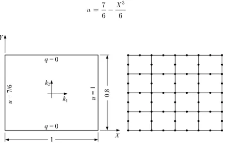
4.1 Example 1: Rectangular temperature field with linear “body force” term

In the first example, we consider a 2D steady-state temperature field over a rectangular domain with length L =1 and width W =0.8 as illustrated in Figure 2. The Dirichlet boundary condi-tions are prescribed on the left and right surfaces, while the Neumann boundary condicondi-tions are specified at the rest of the surfaces. The heat conductivity coefficients are given by k1 =1 and

2 4

k = . In this example, the “body force” term is assumed to be of linear variation along the X direction such that f X,Y

(

)

= -X. This problem admits the analytical solution in the form

3 7

6 6

X

u = - (47)

(11)

As mentioned in Subsection 3.1, the choice of number of Trefftz functions, m, which may affect the accuracy and convergence of the procedure, is an important factor in the practical com-putation. For this purpose 16 elements with 65 nodes are first used to model the entire domain. The results at selected points are listed against different values of m in Table 1, from which it can be seen that large error will appear once m arrives at 18. The reason for this phenomenon is that too many Trefftz functions can result in the numerical overflow when calculating the square matrix H_e. For the best compromise between accuracy and computational effort, the number of Trefftz functions, m =10, is selected in this example. It should be noted that the number of

10

m = is also the optimal one for remaining two examples based on lots of numerical experi-ments.

Coordinates (X_,Y₎

PS-TFEM (RBFs)

Exact

m₌₁₀_{12 14 16 18}

(0.375, 0.400) 1.157881 1.15788 1.15788 1.16125 1.17002 1.15788 -0.07098 -0.07098 -0.07094 -0.07148 -0.04770 -0.07031

(0.500, 0.400) 1.14584 1.14584 1.14584 1.14550 1.15811 1.14583 -0.12409 -0.12409 -0.12374 -0.12225 -0.04512 -0.12500

(0.625, 0.400) 1.12598 1.12598 1.12598 1.13070 1.14013 1.12598 -0.19593 -0.19593 -0.19590 -0.19613 -0.18835 -0.19531

(0.750, 0.400) 1.09636 1.09636 1.09636 1.09514 1.10541 1.09635 -0.28041 -0.28041 -0.28007 -0.28100 -0.09449 -0.28125

1_{data in the 1st row denote the temperature}_u_{and the 2nd row its derivative}_{¶ ¶}_u _X_(similarly

herein-after)

Table 1: Results at selected points for different number, m_{, of Trefftz functions.}

Besides, the convergent performance is also investigated using three meshing densities. As expected, improved numerical accuracy is observed in Table 2 along with an increase in the num-ber of elements.

PS-TFEM (RBFs)

Exact 2×2 mesh 4×4 mesh 8×8 mesh

(0.375, 0.400) 1.15788 1.15788 1.15788 1.15788

-0.07120 -0.07078 -0.07009 -0.07031

(0.500, 0.400) 1.14606 1.14584 1.14583 1.14583

-0.12151 -0.12409 -0.12478 -0.12500

(0.625, 0.400) 1.12637 1.12598 1.12598 1.12598

-0.19615 -0.19574 -0.19510 -0.19531

(0.750, 0.400) 1.09649 1.09636 1.09635 1.09635

-0.28391 -0.28041 -0.28104 -0.28125

Table 2: Convergent performance.

(12)

the distortion parameter l =d r with _r ₌ _L2 ₊_W2 _{. The case of}_l _<₀_{indicates that} ele-ments 6, 7, 10 and 11 distort towards the corner while l >0 indicates that elements 1, 4, 13 and

16 distort towards the center. As a measure of sensitivity to mesh distortion, the relative error defined as below is adopted

distort uniform error

uniform

100%

I I

I

e = - ´ (48)

where Idistort and Iuniform denote the distorted and uniform mesh results, respectively.



25 0.

 

 0 0.25

Figure 3: Scheme for mesh distortion analysis.

Table 3 displays the relative errors for temperature u_{and its derivative}¶ ¶_u _X_{with the} dis-tortion parameter l. Obviously, elements 1, 4, 13 and 16 will become eight-node triangles when

0.125

l= - and the similar trend is for elements 6, 7, 10 and 11 when l =0.125. Once

0.125

l > , the associated elements will collapse to concave quadrilaterals. As is known, it is very intractable or even impossible for conventional isoparametric elements to treat this case be-cause Jacobian matrix will be less than zero when the internal angle of an element is equal to and greater than 180°. This limitation may be easily eliminated by taking the advantage of the “only-boundary integration” Trefftz finite element formulation. It is obviously observed from Table 3 that the relative errors for the temperature u_{are very close to zero, which means the results are} not too sensitive to mesh distortion. Although the maximum relative errors for the temperature derivative ¶ ¶u X at points (0.50, 0.40), (0.25, 0.20) and (0.25, 0.60) reaches -3.425%, 4.647% and 4.647% respectively, the results still meet the request of engineering precision (within 5%).

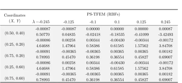
4.2Example 2: Rectangular temperature field with quadratic “body force” term

(13)

to be of quadratic variation in the X_{-direction such that}

(

)

₃ 2

f X,Y = X . For reference, the exact solutions of temperature is given by

4

16

X

u = (49)

PS-TFEM (RBFs)

l=-0.245 -0.125 -0.1 0.1 0.125 0.245

(0.50, 0.40) -0.00087 _0.50770 -0.00087 _0.04835 _-0.024180.00000 _-0.185350.00000 _-0.410990.00000 _-3.424930.00087

(0.25, 0.20) -0.00086 _4.64688 0.00258 _1.47964 0.00344 _0.58386 -0.00430 _0.61585 -0.00344 _1.57562 -0.00172 _3.84708

(0.75, 0.20) -0.00091 _0.78993 -0.00365 _0.45470 -0.00365 _0.36198 0.00365 _0.36554 0.00365 _0.45827 0.00182 _0.69007

(0.25, 0.60) -0.00086 _4.64688 0.00258 _1.47964 0.00344 _0.58386 -0.00430 _0.61585 -0.00344 _1.57562 -0.00172 _3.84708

(0.75, 0.60) -0.00091 _0.78993 -0.00365 _0.45470 -0.00365 _0.36198 0.00365 _0.36554 0.00365 _0.45827 0.00182 _0.69007

Table 3: Relative errors for different mesh distortion parameters.

Figure 4: A rectangular temperature field with quadratic “body force” term.

(14)

2.0 2.5 3.0 3.5 4.0

0 3 6 9 12 15 18

u

X

Theoretical PS-TFEM (RBFs)

Figure 5: Distribution of the temperature u along the top surface.

2.0 2.5 3.0 3.5 4.0

0 10 20 30 40 50 60 70 80

q

Y Theoretical PS-TFEM (RBFs)

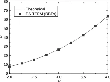
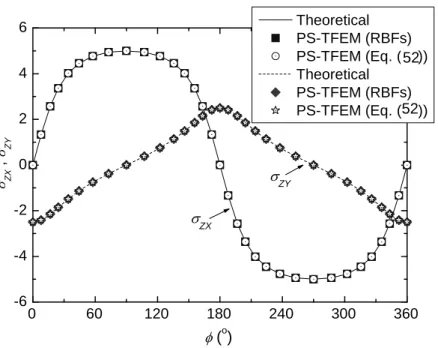
Figure 6: Distribution of the outward normal heat flux q along the right surface. 4.3 Example 3: Torsion of an elliptic shaft

To demonstrate the efficacy of the proposed method for curved geometries, the pure torsion of an elliptic shaft as illustrated in Figure 7 is investigated. The values of semi-major and semi-minor axes are a =10 and b =5. The Dirichlet boundary conditions are prescribed on the outer sur-face of the shaft. In the finite element solution presented, the “body force” term of f X,Y

(

)

= -2

is explored for simplicity. The cross section is represented by a material for which the reciprocal values of shear modulus along the X_{- and}Y_{axes are taken to be}

1 4

k = and k2 =1. This prob-lem admits the analytical solution in the form

2 2 2 2

2 ₄2 1 2 2

a b X Y

u

a b a b

æ _ö÷

ç _÷

= ç -_ç - _÷

÷÷

çè ø

(15)

where the stress function formulation is deduced using the representation for stresses

ZX

u Y s = -¶

¶ , ZY

u X

s = ¶

¶ (51)

One particular solution may be exactly expressed by means of Eq. (12) such that

2 2

1 2 1

2

p

X Y

u

k k

æ _ö÷

ç _÷

= - ç_ç + _÷ ÷÷

çè ø (52)



Figure 7: Torsion of an elliptic shaft.

Figure 8 shows the distribution of stress function u_{along the}X_{- and}Y_{axes. Figure 9 shows} the distribution of shear stresses s_ZX and s_ZY along the outer surface. For clear comparison, the results for shear stresses at selected points are also presented in Table 4. A slight difference was observed between the results based on RBFs and on Eq. (52).

-10 -5 0 5 10

0 4 8 12 16

Y axis

X axis

u

X or Y

Theoretical PS-TFEM (RBFs) PS-TFEM (Eq. (52)) Theoretical

PS-TFEM (RBFs) PS-TFEM (Eq. (52))

(16)

Figure 9: Distribution of shear stresses s_ZXand s_ZY along the outer surface.

u X

¶ ¶ ¶ ¶u Y

RBFs Eq. (52) Exact RBFs Eq. (52) Exact (6.41057, 2.79719) -2.79735 -2.79720 -2.79719 1.60259 1.60265 1.60264 (4.24167, 2.30559) -2.30572 -2.30560 -2.30559 1.06044 1.06042 1.06042 (4.73811, 0.78495) -0.78510 -0.78494 -0.78495 1.18453 1.18454 1.18453 (1.47404, 4.06729) -4.06706 -4.06728 -4.06729 0.36849 0.36851 0.36851 (7.83082, 1.05414) -1.05432 -1.05417 -1.05414 1.95769 1.95777 1.95771 (1.59658, 0.79485) -0.79486 -0.79484 -0.79485 0.39917 0.39915 0.39915 (1.48115, 2.41309) -2.41321 -2.41309 -2.41309 0.37032 0.37029 0.37029 (4.25137, 3.72518) -3.72510 -3.72518 -3.72518 1.06285 1.06285 1.06284

Table 4: A comparison of shear stresses s_ZX and s_ZY between PS-TFEM and exact solutions.

5 CONCLUSIONS

In this paper, we presented a particular solution Trefftz-type finite element approach for solving certain potential problems with “body force” in plane orthotropic materials. The original problem under consideration is first transferred into a homogeneous one using DRM. And then, a modified functional is constructed for the homogeneous orthotropic problem so that the Trefftz-type finite element formulation is derived. In doing so, the advantage ‘only-boundary formulation’ of TFEM is well preserved. Three examples are presented to verify the methodology. It is seen that the approach described in this paper to solve potential problems is, indeed, extremely accurate and robust in comparison with analytical solutions. Although the implementation is carried out for orthotropic potential problems, the idea and development are applicable to anisotropic cases. This work is underway.

0 60 120 180 240 300 360

-6 -4 -2 0 2 4 6

ZX

ZY ZX

,

ZY

 (o)

Theoretical PS-TFEM (RBFs) PS-TFEM (Eq. (55)) Theoretical

PS-TFEM (RBFs) PS-TFEM (Eq. (55))

52

(17)

Acknowledgments

This work has been financed by the Third Visiting Scholar Project from Shanghai Educational Committee. We would like to acknowledge these supports gratefully.

References

Balakrishnan, K., Ramachandran, P.A., (1999). A particular solution Trefftz method for non-linear poisson prob-lems in heat and mass transfer. Journal of Computational Physics 150: 239-267.

Bussamra, F.L.S., Pimenta, P.M., Freitas, J.A.T., (2001). Hybrid-Trefftz stress elements for three-dimensional elas-toplasticity. Computer Assisted Mechanics and Engineering Sciences 8: 235-246.

Cao, L.L., Wang, H., Qin, Q.H., (2012). Fundamental solution based graded element model for steady-state heat transfer in FGM. Acta Mechanica Solida Sinica 25: 377-392.

Cen, S., Zhou, M.J., Fu, X.R., (2011). A 4-node hybrid stress-function (HS-F) plane element with drilling degrees of freedom less sensitive to severe mesh distortions. Computers & Structures 89: 517-528.

Choi, N., Choo, Y.S., Lee, B.C., (2006). A hybrid Trefftz plane elasticity element with drilling degrees of freedom. Computer Methods in Applied Mechanics and Engineering 195: 4095-4105.

Dong, L., Atluri, S.N., (2012a). T-Trefftz Voronoi cell finite elements with elastic/rigid inclusions or voids for mi-cromechanical analysis of composite and porous materials. Computer Modeling in Engineering & Sciences 83: 183-219.

Dong, L., Atluri, S.N., (2012b). Development of 3D T-Trefftz Voronoi cell finite elements with/without spherical voids and/or elastic/rigid inclusions for micromechanical modeling of heterogeneous materials. Computers Materials and Continua 29: 169-211.

Dong, L., Atluri, S.N., (2012c). Development of 3D Trefftz Voronoi cells with ellipsoidal voids and/or elastic/rigid inclusions for micromechanical modeling of heterogeneous materials. Computers Materials and Continua 30: 39-82. Freitas, J.A.T., Ji, Z.Y., (1996). Hybrid-Trefftz equilibrium model for crack problems. International Journal for Numerical Methods in Engineering 39: 569-584.

Fu, Z.J., Qin, Q.H., Chen, W., (2011). Hybrid-Trefftz finite element method for heat conduction in nonlinear func-tionally graded materials. Engineering Computations 28: 578-599.

Jirousek, J., Guex, L., (1986). The hybrid-Trefftz finite element model and its application to plate bending. Interna-tional Journal for Numerical Methods in Engineering 23: 651-693.

Jirousek, J., Qin, Q.H., (1996). Application of hybrid-Trefftz element approach to transient heat conduction analysis. Computers & Structures 58: 195-201.

Jirousek, J., Venkatesh, A., (1992). Hybrid Trefftz plane elasticity elements with p-method capabilities. International Journal for Numerical Methods in Engineering 35: 1443-1472.

Jirousek, J., Wroblewski, A., (1995). A new 12 DOF quadrilateral element for analysis of thick and thin plates. In-ternational Journal for Numerical Methods in Engineering 38: 2619-2638.

Kaczmarczyk, A.L., Pearce, C.J., (2009). A corotational hybrid-Trefftz stress formulation for modelling cohesive cracks. Computer Methods in Applied Mechanics and Engineering 198: 1298-1310.

Kita, E., Ikeda, Y., Kamiya, N., (2005). Sensitivity analysis scheme of boundary value problem of 2D Poisson equa-tion by using Trefftz method. Engineering analysis with boundary elements 29: 738-748.

Leconte, N., Langrand, B., Markiewicz, E., (2010). On some features of a plate hybrid-Trefftz displacement element containing a hole. Finite Elements in Analysis and Design 46: 819-828.

(18)

Nardini, L.C., Brebbia, C.A., (1987). The dual reciprocity boundary element formulation for nonlinear diffusion problems. Computer Methods in Applied Mechanics and Engineering 65: 147-164.

Piltner, R., (1985). Special finite elements with holes and internal cracks. International Journal for Numerical Meth-ods in Engineering 21: 471-1485.

Qin, Q.H., (2000). The Trefftz Finite and Boundary Element Method, WIT Press.

Qin, Q.H., (2003). Solving anti-plane problems of piezoelectric materials by the Trefftz finite element approach. Computational Mechanics 31: 461-468.

Qin, Q.H., (2005). Formulation of hybrid Trefftz finite element method for elastoplasticity. Applied Mathematical Modelling 29: 235-252.

Qin, Q.H., Wang, H., (2008). MATLAB and C Programming for Trefftz Finite Element Methods, CRC Press. Rezaiee-Pajand, M. and Karkon, M. (2012). Two efficient hybrid-Trefftz elements for plate bending analysis. Latin American Journal of Solids and Structures 9: 43-67.

Trefftz, E., (1926). Ein Gegenstuck zum Ritzschen Verfahren. Proceedings of the 2nd International Conference on Applied Mechanics, Zurich, 131-137.

Wang, H., Cao, L.L., Qin, Q.H., (2012). Hybrid graded element model for nonlinear functionally graded materials. Mechanics of Advanced Materials and Structures 19: 590-602.

Wang, H., Qin, Q.H., (2011). Fundamental-solution-based hybrid FEM for plane elasticity with special elements. Computational Mechanics 48: 515-528.

Wang, H., Qin, Q.H., (2012a). Numerical implementation of local effects due to two-dimensional discontinuous loads using special elements based on boundary integrals. Engineering Analysis with Boundary Elements 36: 1733-1745. Wang, H., Qin, Q.H., (2012b). A new special element for stress concentration analysis of a plate with elliptical holes. Acta Mechanica 223: 1323-1340.

Wang, H., Qin, Q.H., Liang, X.P., (2012). Solving the nonlinear Poisson-type problems with F-Trefftz hybrid finite element model. Engineering analysis with boundary elements 36: 39-46.

Wang, K.Y., Huang, Z.M., Li, P.C., Liu, B., (2013). Trefftz finite element analysis of axisymmetric potential prob-lems in orthotropic media. Applied Mathematics and Mechanics 34: 462-469.

Wang, K.Y., Li, P.C., Zhang, M.L., (2012). Trefftz finite element method for orthotropic potential problems. Chinese Quarterly Mechanics 33: 499-506.

Wang, K.Y., Zhang, L.Q., Li, P.C., (2012). A four-node hybrid-Trefftz annular element for analysis of axisymmetric potential problems. Finite Element Analysis and Design 60: 49-56.

Wrobel, L.C., Telles, J.C., Brebbia, C.A., (1986). A dual reciprocity boundary element formulation for axisymmetric diffusion problems. Boundary Elements 44: 1054-1067.

Zhao, X.J., Zhao, J.Y., (2011). Potential problems in anisotropic solids using hybrid finite element model. Chinese Journal of Zhongyuan University of Technology 22: 59-61.