M ESTRADO M ATEMÁTICAF

(1)

M

ESTRADO

M

ATEMÁTICA

F

INANCEIRA

T

RABALHO

F

INAL DE

M

ESTRADO

DISSERTAÇÃO

INTEGRO-DIFFERENTIAL EQUATIONS FOR OPTION

PRICING IN EXPONENTIAL LÉVY MODELS

JOSÉ MANUEL TEIXEIRA DOS SANTOS CRUZ

(2)

M

ESTRADO EM

M

ATEMÁTICA

F

INANCEIRA

T

RABALHO

F

INAL DE

M

ESTRADO

DISSERTAÇÃO

INTEGRO-DIFFERENTIAL EQUATIONS FOR OPTION

PRICING IN EXPONENTIAL LÉVY MODELS

JOSÉ MANUEL TEIXEIRA DOS SANTOS CRUZ

O

RIENTAÇÃO

:

JOÃO

MIGUEL

ESPIGUINHA

GUERRA

(3)

iii

Resumo

Este trabalho discute sob que condi¸cões se pode expressar a fun¸cão que representa o pre¸co de uma op¸cão como solu¸cão de uma determinada equa¸cão integro-diferencial parcial num modelo exponencial de Lévy. A grande diferen¸ca entre o caso aqui considerado e o de Black-Scholes é que existe na equa¸cão um termo não local, o que faz com que a análise seja mais complexa. Também é discutido sob que condi¸cões se pode obter a fórmula de Feynman-Kaˇc para o caso de um processo de saltos puros e sob que condi¸cões o pre¸co de uma op¸cão é solu¸cão clássica de uma equa¸cão integro-diferencial. Quando tais condi¸cões não são verificadas, considera-se o conceito de solu¸cão de viscosidade, que apenas exige que a fun¸cão que representa o pre¸co da op¸cão seja cont´ınua.

Para alguns tipos de processos de Lévy são apresentados resultados de continuidade para os pre¸cos de op¸cões barreira. Para além disso demonstram-se os mesmos resultados para processos de varia¸cão finita e sem componente de difusão. Também são apresentados alguns exemplos em que a fun¸cão que representa o pre¸co da op¸cão é descont´ınua. É apresentado um esquema numérico que permite obter o pre¸co de uma op¸cão de venda Europeia para o caso do processo ”Variance Gamma”. Este esquema de diferen¸cas finitas foi proposto inicialmente por Cont e Voltchkova para resolver numericamente a equa¸cão integro-diferencial parcial associada.

(4)

iv

Abstract

This dissertation discusses under which conditions we can express the function that represents the option price as the solution of a certain partial integro-differential equation (PIDE) in a exponential L´evy model. The main difference between this case and the Black-Scholes case is that there is a non-local term in the equation, which makes the analysis more complicated. Also, we discuss under which conditions we can obtain a Feynman-Kaˇc formula for the case of a pure jump process and discuss the conditions under which option prices are classical solutions of the PIDEs. When such conditions are not verified, we consider the concept of viscosity solutions which only requires that the function representing the option price is continuous.

Continuity results for option prices of barrier options are presented for some types of L´evy processes. In addition, we show the same continuity results for processes of finite variation and with no diffusion component. Also, we present some examples in which the function that represents the option price is discontinuous. Moreover, we present a numerical scheme that gives the price of an European put option for the Variance Gamma process. This finite difference scheme was initially proposed by Cont and Voltchkova, to solve numerically the associated PIDE.

(5)

Acknowledgements

I would like to thank, first of all, my teacher Jo˜ao Guerra, for the help and supervision of the thesis.

Also, i would like to thank to my parents for all the support they gave me all these years. Whithout them, i would not be able to continue my studies.

A special thanks to my brother, Pedro Cruz, for his support and the useful corrections. I thank also to all my family.

(6)

Introduction

One of the main reasons for using the Black-Scholes model is the existence of an analytical formula to price European options. However, evidence from the stock market suggests that this model is not the most realistic one. It is well known that the sample paths of a Brownian motion are continuous, but the stock price of a typical company suffers sudden jumps on an intraday scale, making the price trajectories discontinuous. In the classical Black-Scholes model the logarithm of the price process has normal distribution. However the empirical distribution of stock returns exhibits fat tails. Finally, when we calibrate the theoretical prices to the market prices, we realize that the implied volatility is not constant as a function of strike neither as a function of time to maturity, contradicting this way the prediction of the Black-Scholes model. Several alternatives have been proposed in the literature for the generalization of this model. The models with jumps can, at least in part, solve the problems inherent to the Black-Scholes model. The jump models have also an important role in the options market. While in the Black-Scholes model the market is complete, implying that every payoff can be exactly replicated, in jump models there is no perfect hedge and this way the options are not redundant.

The objective of this thesis is to study under which conditions we can obtain the function that represents the option price as a solution of a certain partial integro-differential equation. Moreover, we will discuss some examples where the price function is not regular enough in order to be a classical solution of this partial integro-differential equation.

The prices of options such as European options and barrier options can be caracterized in terms of solutions of a partial integro differential equation with some boundary conditions depending on the type of option considered. Conversely, if we have a solution of a certain partial integro-differential equation (PIDE) satisfying some conditions, then it is possible to arrive at a stochastic representation of the Feynman-Kaˇc kind, analogous to the Black-Scholes case. The main difference between a model with jumps and the Black-Scholes case is a non-local term that appears in the equation, because now the price process possesses jumps, and the option price can be discontinuous. This non-local term makes PIDEs less easy to solve than partial differential equations. However, one of the numerical schemes used in the literature is presented to solve such equations. In analytical terms, if the price is not a classical (smooth) solution of the PIDE, the notion of viscosity solution can be used.

In Section 2.1 we present the definition of a Lévy process and some notation related to Lévy processes. In Section 2.2 we introduce the Lévy exponential models for financial assets. In Section 2.3 we give some examples of financial models. In Section 3.1 we present the definition of a price of an European option as a discounted expected value of the terminal payoff and a simple derivation of the integro-differential equation whose solution is the discounted expected value of

(8)

2 Chapter 1. Introduction

(9)

Chapter 2

Financial Modelling with L´

evy

Processes

2.1 L´

evy Process: definitions

Let us start with the definition of a L´evy process.

Definition 2.1.1 Consider a fixed probability space (Ω,F,Q). A stochastic process Xt such

that X0 = 0 is called a L´evy process if:

• Xt has independent increments: for every t0 < t1 < .. < tn, the random variables

Xt0, Xt1−Xt0, Xt2 −Xt1, ..., Xtn−Xtn−1 are independent.

• Xt has stationary increments: the law of Xt+h−Xt does not depend ont;

• Xt is stochastically continuous ,i.e. for all a >0 and s >0:

lim

t→sP[|Xt−Xs|> a] = 0

We only consider a right continuous with limits to the left (c´adlag) version ofXtand will denote

∆Xt=Xt−Xt−, the jump of X at timet.

The characteristic function ofXt has the following L´evy-Khintchine representation

([Sat99],[CT04],[App04]):

EeizXt₌_etφ(z)_{, φ}₍_z_{) =}₋σ

2_z2

2 +iγz+

Z +∞

−∞

eizx−1−izx1_|x|≤1

ν(dx).

where σ_≥0 and γ _∈R andν is a positive Radon measure onR_{\ {}0_}verifying:

Z 1

−1

x2ν(dx)<_∞. (2.1)

and _Z

|x|>1

ν(dx)<∞. (2.2)

The measureν is defined by:

ν(A) =E[#_{t_∈[0,1] : ∆Xt∈A}] =

1

TE[#{t∈[0, T] : ∆Xt∈A}], A∈ B(R), (2.3)

(10)

4 Chapter 2. Financial Modelling with L´evy Processes

and is called the L´evy measure of X. It gives the mean number, per unit of time, of jumps whose amplitude belongs to A.

The L´evy-Itˆo decomposition gives a representation whereXis interpreted as a combination of a Brownian motion with drift and a infinite sum of independent compensated Poisson processes with several jump sizes x (see [CT04])

Xt=γt+σWt+

Z t

0

Z

|x|≥1

xJX(ds, dx) +

Z t

0

Z

|x|<1

xJeX(ds, dx), (2.4)

where JX is the Poisson random measure defined in the following way:

JX([0, t]×A) = #{s∈[0, t] : ∆Xs∈A}. (2.5)

The compensated Poisson measure is defined by:

e

JX([0, t]×A) =JX([0, t]×A)−tν(A). (2.6)

A L´evy process is a strong Markov process, the associated semigroup is a convolution semigroup and its infinitesimal generator L : f _→ Lf is an integro-differential operator given by (see [App04]):

Lf(x) = lim

t→0

E[f(x+Xt)]−f(x)

t (2.7)

= σ

2

∂2f ∂x2 +γ

∂f ∂x +

Z

R

f(x+y)−f(x)−y1_|x|≤1

∂f ∂x(x)

ν( dy), (2.8)

which is well defined for f _∈C2(R) with compact support.

2.2 Exponential L´

evy models

Let St be a stochastic process representing the price of a financial asset under a filtered

proba-bility space (Ω,F,{Ft},P). The filtration{Ft}represents the price history up to timet. If the

market is arbitrage-free, then there is a measure Qequivalent to Punder which the discounted prices of all traded financial assets areQ₋martingales. This result is known as the fundamental theorem of asset pricing (see [CT04]). The measureQis also known as the risk neutral measure. We consider here the exponential L´evy model in which the risk-neutral dynamics ofSt underQ

is given bySt=ert+Xt, whereXt is a L´evy process underQwith characteristic triplet (σ, γ, ν).

Then the arbitrage-free market hypothesis imposes that Sbt = Ste−rt = eXt is a martingale,

which is equivalent to the following conditions imposed on the triplet (σ, γ, ν)

Z

|x|>1

eyν( dy)<∞, γ=−σ 2

2 −

Z +∞

−∞

ey−1−y1_|y|≤1

ν(dy). (2.9)

Then the infinitesimal generator (2.8) becomes

Lf(x) =−σ 2

2

∂f ∂x(x) +

σ2

2

∂2f ∂x2 (x) +

Z

R

f(x+y)−f(x)−(ey−1)∂f

∂x(x)

ν( dy) (2.10)

The risk-neutral dynamics of St underQis given by

St=S0+

Z t

0

rSu−du+

Z t

0

σSu−dW_u+

Z t

0

Z

R

(11)

2.3. Examples of L´evy processes in finance 5

The price processStis also a Markov process with state space (0,∞) and infinitesimal generator

(see [CT04])

LSf(x) = lim

h→0

E[f(xeXh_)]₋_f₍_x₎

h (2.12)

=rx∂f ∂x(x) +

σ2x2

2

∂2f ∂x2 (x) +

Z

R

f(xey)₋f(x)₋x(ey₋1)∂f

∂x(x)

ν( dy)(2.13)

2.3 Examples of L´

evy processes in finance

The exponential L´evy models considered in the financial literature are of two types. The first type of models are called jump-diffusion models where we represent the log-price as a L´evy process with a non zero diffusion part (σ >0) and with a jump process with finite activity (i.e

ν(R)<∞). The second type of models are called infinite activity pure jump models in which case there is no diffusion part and only a jump process with infinite activity (i.e ν(R) =_∞).

There are a variety of exponential L´evy models proposed in the financial modelling literature that differ from each other only in the choice of the L´evy measure. In this section we present some examples of models used.

2.3.1 Jump-Diffusion models

A L´evy process of jump-diffusion type is of the following form:

Xt=γt+σWt+ Nt

X

i=1

Yi

where σ > 0, Nt is a Poisson process with intensity λ that counts the jumps of Xt and Yi, i =

1,2,3...are independent and identically distributed random variables with distribution given by

µ. The L´evy measure ν is given by λµ and the drift γ is equal to

−σ 2

2 −

Z

R

ey −1−y1_|y|≤1ν( dy).

2.3.1.1 Merton’s model

This model was introduced by Merton [Mer76] and was the first jump-diffusion model proposed in the financial literature. The random variables Yi, i = 1,2,3...are normally distributed with

mean µand variance δ. Its L´evy density is given by:

ν(x) =λ 1 δ√2πe

−(x−₂δm2)2 (2.14)

Then it’s possible to obtain the probability density of Xtas a series that converges rapidly (see

[CT04]):

pt(x) =

∞

X

j=0

e−λt(λt)j e

−(x₂₍−_σγt2t−+jmjδ2))2

(12)

6 Chapter 2. Financial Modelling with L´evy Processes

Thus, we can express the price of an European call option as a weighted sum of Black-Scholes prices:

CM erton(S0, K, T, σ, r) =e−rT

∞

X

j=0

e−λt(λt)

j

j! e

rjT_C

BS(S0e

jδ2

T , K, T, σ_j, r_j), (2.16)

where rj = r−λ(em+ δ2

2 −1) + jm T , σj =

q

σ2₊jδ2

T and CBS(S, K, T, σ, r) is the well known

Black-Scholes formula.

2.3.2 Infinite activity pure jump models

The Variance Gammma and Normal Inverse Gaussian (NIG) processes are obtained by a subor-dination of a Brownian motion and a tempered α-stable process: the Variance Gamma process correspond toα= 0 and the NIG process corresponds to α= 1/2. These models are popular in the literature beacuse the probability density of the subordinator is known in a closed form for those values of α (see [CT04]).

2.3.2.1 Variance Gamma Process

The Variance Gamma process is a pure discontinuous process of infinite activity and finite variation (R_|_x_|≤₁|x|ν( dx)<∞) that is widely used in the financial modelling. Its L´evy measure is given by

ν(x) = 1

κ_|x_|e

Ax−B|x| _with_A₌ θ

σ2 and B =

q

θ2_{+ 2}σ2 κ

σ2 ,

whereσ and θare parameters related with the volatility and drift of the Brownian motion with drift and κ is the parameter related with the variance of the subordinator, in this case the Gamma process (see [CT04]). The probability density is given by

pt(x) =CeAx|x| t kKt

k−

1 2(|x|),

where K is the modified Bessel Function of second kind. The characteristic function ofXt+γtis equal to :

Φt(u) =eituγφt(u) =eituγ

1 +σ

2_u2_κ

2 −iθκu

−t/κ

,

where γ is determined by the martingale condition and φt(u) is the characteristic function of

Xt. In fact, we must have

E[e−rTST|Ft] =e−rtSt, (2.17)

where

St=S0ert+γt+Xt (2.18)

(13)

2.3. Examples of L´evy processes in finance 7

2.3.2.2 Normal Inverse Gaussian model

The NIG process is a process of infinite activity and infinite variation without any Brownian component. Its L´evy measure is given by (see [CT04])

ν(x) = C

|x|e

Ax_K

1(B|x|)

and

C=

q

θ2₊σ2 κ

2πσ√κ , A= θ σ2, B=

q

θ2₊σ2 κ

σ2 ,

where θ,σ and κ have the same meaning as in the Variance Gamma process. The probability density is:

pt(x) =CeAx

K1(B

q

x2₊t2_σ2 κ )

q

x2₊t2_σ2 κ

whereK is the modified Bessel Function of second kind. The characteristic function is given by

Φt(u) =e t κ−

t κ

√

1+u2_σ2_κ₋₂_iuθκ

. (2.19)

2.3.2.3 Generalized Hyperbolic model

The Generalized Hyperbolic model is a process of infinite variation whithout gaussian part. Its characteristic function is given by (see [CT04])

φt(u) =eiµu(

α2₋β2 α2₋₍_β₊_iu₎2)

t

2κ

Kt κ(δ

p

λ2₋₍_β₊_iu₎2₎

Kt κ(δ

p

α2₋_β2₎ , (2.20)

where δ is a scale parameter, µis the shift parameter and κ has the same meaning that in the Variance Gamma process. The parameters λ,α and β determine the shape of the distribution. The density function

pt(x) =C(

p

δ2_{+ (}_x₋_µ₎2₎kt−

1 2Kt

κ−

1 2(α

p

δ2₋₍_x₋_µ₎2₎_eβ(x−µ)_,

where K is the modified bessel function and

C = (

p

α2₋_β2₎kt

√

2πακt−12δ

t κKt

κ(δ

p

α2₋_β2₎.

(14)

Chapter 3

Integro-differential equations for

option pricing

3.1 Definitions

The value of a European option is defined as the discounted conditional expectation of the terminal payoff H(ST) under the risk neutral probabilityQ:

Ct=C(t, St) =E

h

e−r(T−t)H(ST)|Ft

i

=Ehe−r(T−t)H(ST)|St=S

i

=e−r(T−t)E[H(Ser(T−t)+XT−t_)]_,

because of the Markov property and the fact that Xtis a L´evy process.

IfH is in the domain of the infinitesimal generatorLS, then if we differentiateC(t, St) with

respect tot ,we obtain the following integro-differential equation

∂C

∂t (t, S) +L

S_C₍_{t, S}₎₋_rC₍_{t, S}_{) = 0;}_C₍_{T, S}_{) =}_H₍_S₎_, _(3.1)

where LS _{is defined by (2.13).}

Definingτ =T₋t, x=ln_SS

0

, h(x) =H(S0ex) andf(τ, x) =erτC(T −t, S0ex) we get

f(τ, x) =EH Serτ+Xτ₌_E_{H S}

0ex+rτ+Xτ=E[h(x+rτ +Xτ)]. (3.2)

The associated infinitesimal generator is given by (2.10). Then, similarly to the previous case, differentiating (3.2) with respect to τ we obtain the integro-differential equation

∂f

∂τ =Lf +r ∂f

∂x,(τ, x)∈(0, T]×R; (3.3)

(15)

3.2. Feynman-Kaˇc formula for PIDEs 9

Indeed, by the definition of the associated infinitesimal generator we get

Lf(x) = lim

k→0

E[f(τ, x+Xk)]−f(τ, x)

k

= lim

k→0

E[h(x+rτ+Xk+τ)]−E[h(x+rτ +Xτ)]

k

= lim

k→0

E[h(x+r(τ+k) +Xk+τ)]−E[h(x+rτ+Xτ)]

k

− lim

k→0

E[h(x+r(τ +k) +Xk+τ)]−E[h(x+rτ+Xk+τ)]

k

= ∂f

∂τ −klim→0

E[h(x+r(τ+k) +Xk+τ)]−E[h(x+rτ+Xk+τ)]

k

= ∂f

∂τ −zlim→0r

E[h(x+z+rτ +Xz

r+τ)]−E[h(x+rτ +X z r+τ)]

z =

∂f ∂τ −r

∂f ∂x.

3.2 Feynman-Kaˇ

c formula for PIDEs

For t≥0, let Ft denote the σ−algebra generated by the random variables {Xs,0≤s≤t} and

H_T2 =

φt, t∈[0, T] :kφk2=E[

Z T

0 |

φt|2dt]<∞

M2

T is the subspace of HT2 that contains predictable processes. Let HT2(l2) andMT2(l2) denote

the corresponding spaces of l2-valued processes equipped with the norm:

kφk2=E[

Z T

0

∞

X

i=1

|φ(_ti)|2dt].

Finally set H2

T =HT2 ×MT2(l2).

Following Nualart and Schoutens [NS00], they define the power-jump processes for every

i= 1,2,3, ...., nX_t(i), t≥0oand the compensated power-jump processes or Teugel martingales

n

Yi

t =Xti−E

h

X_t(i)i, t_≥0o, in the following way:

X_t(1)=Xt,

X_t(i)= X

0<s≤t

(∆Xs)i, i= 2,3,4, ....,

Y_t(i)=X_t(i)₋tEhX_t(i)i, i_≥1,

Then applying a orthonormalization procedure to the martingalesY(i)we obtain a set of pairwise strongly orthonormal martingales H(i)_{, t}_≥₀ _{, i} _{= 1}_,₂_{, ....} _{such that each} _H(i) _{is a linear}

combination of theY(j)_{, j}_{= 1}_,₂_{, ...i}_:

H(i)=ci,iY(i)+...+ci,1Y(1),

where

c1,1 = [

Z

R

(16)

10 Chapter 3. Integro-differential equations for option pricing

and

E[X1] =a+

Z

|x|≥1

xν(dx).

The constants ci,j are the orthonormalization coefficients of the polynomials 1, x, x2, x3, ....

with respect to the measure µ(dx) =x2ν(dx) +σ2δ0(dx) and the polynomials we want to find

are of the form

qi−1(x) =ci,1+ci,2x+ci,3x2+...+ci,i−1xi−2+ci,ixi−1, i= 1,2,3....

Then, we just have to multiply byxto get the desired pairwise strongly orthonormal martingales:

pi(x) =ci,1x+ci,2x2+ci,3x3+...+ci,i−1xi−1+ci,ixi, i= 1,2,3....

We now see that:

H_t(i) =pi(Y(i)).

An important result in Nualart and Schoutens [NS00] is the predictable representation property:

Theorem 3.2.1 Let F _∈L2_(Ω_,_F

T,P).Then F has a representation of the form:

F =E[F] +

∞

X

j=1

Z T

0

φ_t(j)dH_t(j) where φ(_tj) (3.5)

are predictable processes such that

E[

Z T

0

∞

X

j=1

|φ(_tj)|2dt]<∞. (3.6)

Consider the Backward Stochastic Differential Equation (BSDE):

−dYt=b(t, Yt−, Z_t) dt−

∞

X

i=0

Z_t(i)dH_t(i), YT =ξ (3.7)

whereH_t(i)is the orthonormalized Teugel martingale of orderiassociated with the L´evy process X,b: Ω×[0, T]×R_×M_T2(l2)→Ris a measurable function and uniformly Lipschitz in the first two components and ξ _∈L2_T.

Consider the particular case of a BSDE:

dYt=

∞

X

i=0

Z_t(i)dH_t(i), YT =h(XT) (3.8)

Let f(τ, x) be the solution of the following PIDE:

∂f ∂τ =c

∂f ∂x +

Z

R

f(τ, x+y)₋f(τ, x)₋y∂f ∂x

ν( dy),

(17)

3.2. Feynman-Kaˇc formula for PIDEs 11

Definingg(t, x) =f(τ, x), whereτ =T ₋t , we obtain from (3.9):

∂g ∂t +c

∂g ∂x+

Z

R

g(t, x+y)₋g(t, x)₋y∂g ∂x

ν( dy) = 0,

g(T, x) =h(x) (3.10) If g is sufficiently smooth, then by applying the Itˆo formula tog(t, Xt) we obtain the following

probabilistic representation for the case of a L´evy process given by Xt = (r +γ)t+ Jt =

a+Jt,where Jt is a pure jump process. For a detailed proof of this proposition see [NS01]. Proposition 3.2.1 Assume σ = 0 and _∃λ >0 such that

Z

|x|>1

eλ|x|ν(dx)<_∞.

If g∈C1,2 is a classical solution of (3.10)and ∂g_∂x and ∂_∂x2g2 are bounded by a polynomial function

of x, uniformly in t, then the unique adapted solution of (3.8)is given by

Yt=g(t, Xt),

where

Z_t1=

Z

R

g(t, X_t−+y)−g(t, X_t−)−y

∂g

∂x(t, Xt−)

p1(y)ν( dy) +

∂g

∂x(t, Xt−)

Z

R

y2ν( dy)

1/2

,

Z_ti=

Z

R

g(t, Xt−+y)−g(t, X_t−)−y∂g

∂x(t, Xt−)

pi(y)ν( dy), i≥2

and g(t, x) =E[h(XT)|Xt=x].

The probabilistic representation

g(t, x) =E[h(XT)|Xt=x] (3.11)

obtained in the previous proposition is a Feynman-Kaˇc formula for the solution of the PIDE (3.10).

Sketch of the proof. We can apply Itˆo’s formula for processes with jumps, presented in Proposition 8.19 of [CT04], to g(s, Xs) froms=ttos=T:

g(T, XT) =g(t, Xt) +

Z T

t

∂g

∂t(s, Xs−) ds+

Z T

t

∂g

∂x(s, Xs−) dXs

+ X

t<s≤T

[g(s, Xs)−g(s, Xs−)−

∂g

∂x(s, Xs−)∆Xs]. (3.12)

Making use of Lemma 5 in [NS00] and applying it to h(s, y) = g(s, Xs)−g(s, Xs− +y) −

∂g

∂x(s, Xs−)y we get,

g(T, XT) =g(t, Xt) +

Z T

t

∂g

∂t(s, Xs−) ds+

Z T

t

∂g

∂x(s, Xs−) dXs

+ ∞ X i=1 Z T t Z R

(g(s, Xs)−g(s, Xs−+y)−

∂g

∂x(s, Xs−)y)pi(y)ν( dy) dH

(i)

s + Z T t ( Z R

g(s, Xs)−g(s, Xs−+y)−

∂g

(18)

But Xt=Yt(1)+tE[X1] = (R_Ry2ν( dy))1/2Ht(1)+t(a+

R

|y|≥1yν( dy)), so

h(XT) =g(t, Xt) +

Z T

t

[∂g

∂t(s, Xs−) +

Z

R

(g(s, Xs)−g(s, Xs−+y)− ∂g

∂x(s, Xs−)y)ν( dy)

+ (a+

Z

|y|≥1

yν( dy))∂g

∂x(s, Xs−)] ds+

Z T

t

∂g

∂x(s, Xs−)(

Z

R

y2ν( dy))1/2dH_s(1)

+ ∞ X i=1 Z T t ( Z R

(g(s, Xs)−g(s, Xs−+y)−

∂g

∂x(s, Xs−)y)pi(y)ν( dy)) dH

(i)

s . (3.14)

Then because g(t, x) solves (3.9) and taking expectations in (3.14), we get:

g(t, x) =E[h(XT)|Xt=x].

The next example shows how to perform the orthonormalization procedure described above and presents the Feynman-Kaˇc formula for a pure jump process.

Example 3.2.2 Consider the case where we have the sum of two compensated Poisson pro-cesses, Xt =Nt1+Nt2 where Nt1 = Nt−λ1t and Nt2 =Nt−λ2t, with L´evy measure ν(dx) =

(λ1+λ2)δ1(x) dx. Then performing a orthonormalization procedure we get

ψ0= 1⇒q0 =

1

(R_Rx2_ν₍_dx₎₎1/2 =

1 (R_Rx2₍_λ

1+λ2)δ1(x) dx)1/2

= 1

(λ1+λ2)1/2

ψ1=x+a1,0q0⇒ψ1 =x− hx, q0iq0 =x−

Z

R

x_√ 1 λ1+λ2

(λ1+λ2)x2δ1(x)

1

√

λ1+λ2

dx

=x₋1_⇒ψ1 = 0⇒q1 = 0.

By recurrence we get that qi = 0, i = 1,2,3, ... . Then in terms of previous notation p1(x) =

x

√

λ1+λ2 andpi(x) = 0, i= 2,3, ..., which implies

H_t(1) = √ 1

λ1+λ2

Xt and Ht(i)= 0, i= 2,3, .... (3.15)

Then, by Proposition (3.2.1)

Yt=h(XT)−

Z T

t

Z_s(1)dH_s(1),

where

Z_t(1) = [g(t, x+ 1)−g(t, x)− ∂g

∂x]

p

λ1+λ2+∂g

∂x

p

λ1+λ2 = [g(t, x+ 1)−g(t, x)]

p

λ1+λ2.

Then,

Yt=h(XT)−

Z T

t

[g(t, X_s−+ 1)−g(t, X_s−)]

p

λ1+λ2

1

√

λ1+λ2

dXs⇔

Yt=h(XT)−

Z T

t

[g(t, X_s−+ 1)−g(t, X_s−)] dX_s.

Moreover,

(19)

3.3. Option prices as classical solutions of PIDEs 13

Notice that in Proposition 3.2.1, g is assumed to be smooth and its derivatives have to be bounded by a polynomial function of x, uniformly in t. However, these conditions are rarely satisfied in applications.

Example 3.2.3 Consider an European call option with payoff function H(x) = (x−1)+ and strike price K = 1. We see that the first derivative of the payoff function has a discontinuity at

x= 1:

H′(x) =

1 if x >1,

0 if x <1

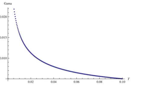
Then, we see that the second derivative diverges at x = 1. So, when t tends to T and if the option is at the money (S =K) the second derivative of the price function tends to the second derivative of the payoff function that diverges when S=K. This means that the gamma of the call option is not uniformly bounded in time.

0.02 0.04 0.06 0.08 0.10

T

0.010 0.015 0.020

Gama

Figure 3.1: As T tends to zero the gamma of the option tends to infinity.

3.3 Option prices as classical solutions of PIDEs

3.3.1 European Options

Consider an European option with maturity T and payoff H(ST).Assume that the payoff

func-tion is a Lipschitz funcfunc-tion

|H(x)₋H(y)_{| ≤}c_|x₋y_| (3.17) for somec >0. As we already know, the value of that option at timet is :

C(t, St) =E

h

e−r(T−t)H(ST)|St=S

i

=e−r(T−t)EhHSer(T−t)+XT−ti_. _(3.18)

We will assume thatSbt=eXt is a square integrable martingale

Z

|x|>1

(20)

Then the dynamics of Sbt is given by:

dSbt

b

S_t−

=σdWt+

Z

R

(ex₋1)JeX(dt, dx), sup t∈[0,T]

EhSb_t2i<_∞. (3.20) The proofs of the following propositions are presented in [Vol05] and are shown in greater detail in the appendix. These propositions will be needed to prove the Proposition 3.3.3.

Proposition 3.3.1 Let the payoff function H satisfy the Lipschitz condition (3.17). Then the forward value of an European option defined by (3.2),f(τ, x) =E[H(Sex+rτ+Xτ_)]_{, is continuous}

on [0, T]×R.

Proposition 3.3.2 Let h be a measurable function with polynomial growth at infinity: _∃p >

0,_|h(x)_{| ≤}C(1 +xp₎_{. If}

σ >0 or _∃β _∈(0,2) such that lim

ǫ→0inf

1

ǫ2−β

Z ǫ

−ǫ|

x_|2ν( dx)>0 (3.21)

and

∀n_≥0,

Z

|y|>1|

y_|nν( dy)<_∞, (3.22)

Then, f(τ, x) =E[h(x+rτ+Xτ)] belongs toC∞((0, T]×R).

The proof of this proposition, following the proof given in Voltchkova [CV05b], is presented here in greater detail.

Proposition 3.3.3 Consider the exponential L´evy model St=S0ert+Xt where the L´evy process X verifies (3.19) and (3.21). Then the value of a European option with terminal payoff H(ST)

(satisfying (3.17)) given by

C: [0, T]×(0,∞)→R,(t, S)→C(t, S) =Ehe−r(T−t)H(ST)|St=S

i

(3.23)

is continuous on [0, T]×(0,∞), C∞ on (0, T) ×(0,∞) and satisfies the integro-differential equation:

∂C

∂t (t, S) +rS ∂C

∂S (t, S) + σ2_S2

2

∂2_C

∂S2 (t, S)−rC(t, S) +

+

Z

C(t, Sey)−C(t, S)−S(ey−1)∂C

∂S (t, S)

ν( dy) = 0; (3.24)

on [0, T)×(0,∞) with the terminal condition:

C(T, S) =H(S) ,_∀S >0 (3.25)

Proof. By Proposition 3.3.1 we know thatC(t, S) =erτ_f₍_{τ, x}_{) is continuous on [0}_{, T}_]_×_R_and

by Proposition 3.3.2, C(t, St)∈C∞((0, T)×(0,∞)).

It remains to prove thatC(t, S) satisfies (3.24). The risk neutral dynamics ofSt under Qis given by

dSt=rSt−dt+σS_t−dW_t+

Z

R

(21)

Applying the Itˆo formula to Cbt = e−rtC(t, St) where St = ert+Xt we get (see Proposition

8.18 of [CT04])

d(e−rtC(t, St)) =e−rt(−rC(t, St−) dt+

∂C

∂t(t, St−) dt+ σ2

2 S

2

t−

∂2_C

∂S2(t, St−) dt

+∂C

∂S(t, St−) dSt+

Z

R

(C(t, y+S_t−)−C(t, S_t−)−y

∂C

∂S(t, St−))JeS(dt, dy)).

simplifying and plugging in the dynamics for St we get:

dCbt=e−rt

∂C

∂S(t, St−)σSt−dWt+e−

rtZ

R

(C(t, S_t−ex)−C(t, S_t−))Je_X(dt, dx)

+e−rt(₋rC(t, S_t−) +

∂C

∂t(t, St−) + σ2

2 e−

rt_S2

t−

∂2C

∂S2(t, St−) +rSt−

∂C

∂S(t, St−)

+

Z

R

(C(t, S_t−ex)−C(t, S_t−)−S_t−(ex−1)

∂C

∂S(t, St−))ν( dx)) dt

=b(t) dt+ dMt.

where

b(t) =−rC(t, S_t−) +∂C

∂t(t, St−) + σ2

2 e

−rt_S2

t−

∂2C

∂S2(t, St−) +rSt−

∂C

∂S(t, St−)

+

Z

R

(C(t, S_t−ex)−C(t, S_t−)−S_t−(ex−1)

∂C

∂S(t, St−))ν( dx),

Mt=

Z T

0

e−rt∂C

∂S(t, St−)σSt−dWt+

Z T

0

e−rt

Z

R

(C(t, S_t−ex)−C(t, S_t−))Je_X(dt, dx).

It remains to prove thatMtis a martingale, because by proposition 8.9 of [CT04], ifCbt−Mt=

Rt

0b(s) dsis a continuous martingale with finite variation paths then

Rt

0b(s) ds=X0 a.s, which

implies that b(t)=0 a.s.

In order forR₀te−rtR_R(C(t, S_t−ex)−C(t, S_t−))Je_X(dt, dx) to be a martingale we have to show

that:

E[

Z T

0

e−2rt

Z

R

(C(t, S_t−ex)−C(t, S_t−))2ν( dx) dt]<∞.

Then, by the Lipschitz condition

E[

Z T

0

e−2rt

Z

R

(C(t, S_t−ex)−C(t, S_t−))2ν( dx) dt]≤E[

Z T

0

e−2rt

Z

R

c2S_t2−(ex−1)2ν( dx) dt].

Moreover,

c2

Z

R

(ex−1)2ν( dx) =c2

Z

|x|≤1

(ex−1)2ν( dx) +c2

Z

|x|>1

(ex−1)2ν( dx)

≤ek2

Z

|x|≤1|

x_|2ν( dx) +c2

Z

|x|>1

(ex₋1)2ν( dx)

=ek2

Z

|x|≤1|

x_|2ν( dx) +c2

Z

|x|>1

(e2x+ 1₋2ex)ν( dx)

≤ek2

Z

|x|≤1|

x|2ν( dx) +ek2

Z

|x|>1

(22)

for someek sufficiently big. Then,

E[

Z T

0

e−2rt

Z

R

c2S_t2−(ex−1)2ν( dx) dt]

≤E[

Z T

0

S_t2−e−2rt ek2

Z

|x|≤1|

x_|2ν( dx) +ek2

Z

|x|>1

(e2x+ 1)ν( dx)

!

dt]

=ek2

Z

|x|≤1|

x_|2ν( dx) +

Z

|x|>1

(e2x+ 1)ν( dx)

!

E[

Z T

0

S_t2−e−2rtdt]

=ek2

Z

R

1∧ |x|2ν( dx) +

Z

|x|>1

e2xν( dx)

! Z T

0

E[S_t2−]e−2rtdt <∞.

Then R₀te−rtR

R(C(t, St−ex)−C(t, St−))JeX(dt, dx) is a square integrable martingale. It remains to prove thatR₀T e−rt ∂C_∂S(t, S_t−)σS_t−dW_t is also a martingale, such thatM_t is a

martingale.

E[

Z T

0

e−2rt(∂C

∂S(t, St−)σSt−)

2_d_t_]_≤_E_[Z T 0

e−2rt

∂C

∂S(t, St−)

2 L∞

σ2S_t2−dt]

≤c2σ2

Z T

0

e−2rtE[S_t2−] dt <∞,

because if C is Lipschitz, then ∂C_∂S(t, St−)∈L∞.

The condition (3.21) holds for all jump-diffusion models with Brownian component or for processes with L´evy densities with behavior near zero asν(x)_∼ _x1+cβ withβ >0. This condition

is not satisfied for the Generalized Hyperbolic model or in particular for the Variance Gamma model. The next example shows that if we do not impose any conditions on a given L´evy triplet, then the function that represents the price of a binary option is not smooth.

Example 3.3.1 Consider the Generalized Hyperbolic model and for simplicity assume δ = 0. Then the density function becomes

pt(x) =C|x−µ| t κ−

1 2K

|κt−

1

2|(α|x−µ|)e β(x−µ)_.

Notice that, when

z_→0 , Kv(z)∼

1 2Γ(v)(

z

2)−

v _⇒

lim

x→µp(t, x) = limx→µC|x−µ| t κ−

1 2K

|kt−

1

2|(α|x−µ|)e β(x−µ)

= lim

x→µC|x−µ| t κ− 1 2−| t κ− 1 2|1

2Γ(

t κ −

1 2)e

β(x−µ)₌_∞

if and only if

t κ −

1 2 − |

t κ −

1

2|<0⇔2(

t κ −

1 2)<0.

Then we conclude that p(t, x) is locally unbounded at x=µ if t < κ₂.

If 0< t κ −

1 2− |

t κ −

1

2|<1 , then p(t, x)∈C

0 _{but not in} _C1_.

If 0< t κ −

1 2− |

t κ −

1

2|<1 or 1<2

t

κ <2 , then p(t, x)∈C

0 _{but not in} _C1_.

If 1< t κ −

1 2− |

t κ −

1

2|<2 or 2<2

t

κ <3 , then p(t, x)∈C

(23)

So by recurrence we conclude that

if p−1< t κ −

1 2− |

t κ −

1

2|< p or p <2

t

κ < p+ 1, then p(t, x)∈C

p−1 _{but not in}_Cp_.

So if t _∈ (pκ₂,(p+ 1)κ₂) then p(t, x) belongs to Cp−1₍_R₎ _{but not in} _Cp₍_R₎ _{and for} _{t <} κ

2,

p(t, .) is locally unbounded.

1.0 1.5 2.0

S

0.2 0.4 0.6 0.8 1.0

Price

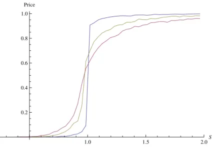
Figure 3.2: The price of a binary option is not differentiable at the money, using the Monte Carlo method, when µ= 0 with κ = 2, r= 0, σ= 0.25, θ =−0.1. Blue: T = 0.1, red: T = 0.5, yellow: T = 1.

Consider a binary option whose payoff function is given by h(x) = 1x≥l0. Its price is given

by

C(t, S) =e−r(T−t)E[H(ST)|St=S] =e−r(T−t)E[h(x+r(T−t) +XT−t)]

=e−r(T−t)E[1_x₊_r₍_T₋_t₎₊_X_T₋_t_≥_l₀] =e−r(T−t)Q[x+r(T₋t) +XT−t≥l0]

=e−r(T−t)Q[XT−t≥l0−r(T −t)−x] =

Z _∞

d

p(t, x) dx.

(24)

3.3.2 Barrier Options

We now present the result without proof, analogous to Proposition 3.3.3. It tells us that the price function of a barrier option is smooth enough if and only if it satisfies a PIDE. For a full detailed proof of this proposition see [Vol05].

Proposition 3.3.4 Consider St=S0ert+Xt where the L´evy process X verifies (3.19). Let θt=

inf{s≥t|St∈/ (L, U)} where 0 ≤L < U ≤ ∞ and suppose that H ≥ 0 and ∃N > 0 : H(S) ≤

N(1 +S). Define

Cb(t, S) =e−r(T−t)E[H(ST)1T <θt|St=S], (3.26)

as the value of a knock-out option, where Cb(t, S) ∈ C1,2([0, T)×(L, U)). Then it satisfies the

integro-differential equation:

∂Cb

∂t (t, S) +rS ∂Cb

∂S (t, S) + σ2S2

2

∂2Cb

∂S2 (t, S)−rCb(t, S) +

+

Z

Cb(t, Sey)−Cb(t, S)−S(ey−1)

∂Cb

∂S (t, S)

ν( dy) = 0; (3.27)

on [0, T)×(L, U) with the conditions:

Cb(T, S) =H(S) ∀S ∈(L, U), (3.28)

Cb(t, S) = 0 ∀S /∈(L, U). (3.29)

Conversely, every solution of(3.27)₋(3.29)belonging to C1,2_([0_{, T}₎_×₍_{L, U}₎₎_{has the stochastic} representation given by (3.26).

Before we study the continuity of barrier option prices we will need the definition of first passage process: Let {Yt} be a L´evy process defined by Yt = rt+Xt. Finally set Mt = sup0≤s≤tYs.

Following the notation of Sato [Sat99], we define

Rx = inf{s≥0|Ys > x}, R−x = inf{s≥0| −Ys> x},

R′′_x = inf_{s_≥0_|Ys∨Ys−≥x}.

We know that _{Rx, x≥0} is a process with non-decreasing paths, so we can defineRx−(ω) =

limǫ→0Rx−ǫ(ω). As for the right continuity, since Yt is right-continuous, Rx is also

right-continuous. Following the terminology of Voltchkova:

Definition 3.3.2 Consider a L´evy processYt with triplet (σ, γ, ν).

If σ= 0 and ν(R)<_∞, then Yt is of type A (Compound Poisson).

If σ = 0, ν(R) = _∞ and R_|_x_|≤₁_|x_|ν( dx) <_∞, then Yt is of type B (finite variation,infinite

activity).

If σ >0 or R_|_x_|≤₁_|x_|ν( dx) =_∞, then Yt is of type C (infinite variation) .

In order to prove the continuity of barrier option prices we need some properties of the process_{Rx}.

(25)

Lemma 3.3.3 If _{Yt} is of type B or C or A with γ 6= 0 then:

∀x >0,Q[R_x− =R_x] = 1. (3.30)

Proof.

Introducing

Ω1 ={ω ∈Ω :Rx− < R_x},Ω₂ =

n

ω _∈Ω :R′′_x =Rx

o

.

Define R_x′ = inf{s≥0|Y_s≥x} By Lemma 49.6 of [Sat99] we have that, for any x >0,P[R_x =

R_x′ = R ′′

x] = 1, because Yt is non zero and is not Compound Poisson process, which means

that is of type B or C or A with γ ₆= 0. Then Q[Ω2] = 1. In order that, Q[Rx− = R_x] = 1

we must have Q[Ω1] = 0, because we always have Rx− ≤ R_x. So we have to prove that

Q[R_x− < R_x] =Q[R_x−< R ′′

x] =Q[Ω1∩Ω2] = 0.

By contradiction, suppose that _∃ω_∈Ω1∩Ω2 ⇒ω∈Ω1, ω∈Ω2.Then,

∃u≥0, R_x− =u (3.31) ∃u< t, t=R_x′′. (3.32)

By definition ofR_x− = lim_ǫ_→₀, R_x₋_ǫ and becauseR_x− =u we get,

∀δ>0,∃η>0 :|ǫ|< η ⇒u−δ < Rx−ǫ < u+δ.

∀ǫ>0,∀δ>0,∃s < u+δ :Ys > x−ǫ.

Now, choose ǫn=δn= 1_n →0.Then,

∃sn∀n:sn< u+

1

n, Ysn > x−

1

n.

Because _{sn} is bounded, there is a convergent subsequencesnk ↑s0 withs0 ≤u < t. This

means that,

Ysn > x−

1

n ⇒Ys−₀ ≥x.

and if snk ↓s0 withs0≤u < t,then

Ysn > x−

1

n ⇒Ys0 ≥x.

Then,Y_s−

0 ∨Ys0 ≥x. But this contradicts (3.32) because it implies that∀s < t,Ys−∨Ys< x.

Then Ω1∩Ω2 =∅.

Lemma 3.3.4 If {Yt} is of type B with R0= 0 a.s or of type C, then:

∀x >0,_∀t_≥0,Q[Rx=t] = 0. (3.33) Lemma 3.3.5 If _{Yt} is of type B or C, then ∀x >0,∀t≥0 :

Q[Rx≤t < Rx+ǫ]→0, (3.34)

Q[Rx−ǫ≤t < Rx]→0, (3.35)

(26)

The next proposition shows that the up-and-out option is continuous. The sketched proof of this proposition is shown in [Vol05] and a more detailed version is shown in the appendix.

Proposition 3.3.5 Let Yt be of type B or C with R0 = 0 a.s. Suppose that H: (0, U)→[0,∞) is Lipschitz:

∀S1, S2∈(0, U),|H(S1)−H(S2)| ≤k|S1−S2|, (3.36) for some k >0 and let u=log(_SU

0). Then the function fU(τ, x) defined by

fU(τ, x) =

EH S0ex+Yτ1τ <Ru−x

if x < u,

0, if x_≥u (3.37)

is continuous on (0, T]_×R.

The following proposition gives the continuity result for the case of a down-and-out option. The proof of this proposition, similar to the previous one, can be found in [Vol05].

Proposition 3.3.6 LetYtbe of type B or C withR0− = 0a.s. Suppose thatH : (L,∞)→[0,∞)

is Lipschitz:

∀S1, S2∈(0, U),|H(S1)−H(S2)| ≤k|S1−S2|, (3.38) with L < S0 and let l=log(_SL₀). Then the function fL(τ, x) defined by

fL(τ, x) =

(

EhH S0ex+Yτ1_{τ <R}−

x−l

i

if x > l,

0, if x≤l (3.39)

is continuous on (0, T]×R.

Finally the continuity result of a double-barrier option with payoffH(ST)1T <inf{t≥0,St∈(L,U)},

where L < S0 < U, u = log(_SU₀) and l = log(_SL₀) is presented here without proof and can be

found in [Vol05].

Proposition 3.3.7 Let Yt be of type B or C with R0− = 0 and R₀ = 0 a.s. Suppose that

H : (L,_∞)_→[0,_∞) is Lipschitz:

∀S1, S2∈(0, U),|H(S1)−H(S2)| ≤k|S1−S2|, (3.40) with k >0.Then the function fD(τ, x) defined by

fD(τ, x) =

(

x−l∩Ru−x

i

if x_∈(l, u),

0, if x /_∈(l, u) (3.41)

is continuous on (0, T]_×R.

The results for the continuity of a up-and-out option and a down-and-out option are proven here when the L´evy process is of type A.

Proposition 3.3.8 Suppose _{Yt} is a L´evy process of type A with γ 6= 0, R0 = 0 a.s and

Q[Rx = t] = 0,∀x ≥0, t ≥0,(t, x) 6= (0,0). Suppose that H:(0, U) → (0,∞) is Lipschitz.Then

for every τ sufficiently small fu(τ, x) defined by

fu(τ, x) =

EH S0ex+Yτ1τ <Ru−x

if x < u,

0 if x≥u

(27)

Proof. Consideringτ >0 andx=u, we have by definition,

|fu(τ, u−ǫ)−fu(τ, u)|=EH S0eu−ǫ+Yτ1τ <Rǫ

≤M E[1τ <Rǫ] =MQ[τ < Rǫ]

Let_{ǫn} →0 and Ωn={ω∈Ω :τ < Rǫn}, then{Ωn}is a decreasing sequence: Ω1 ⊃Ω2 ⊃

...Ωn⊃..., becauseRx is an increasing process. Then

lim

n→∞Q[τ < Rǫn] =Q[∩ ∞

n=1Ωn] =Q[τ < R0] = 0

because R0 = 0 a.s.

Forτ >0 andx < u:

|fu(τ, x+ǫ)−fu(τ, x)|=|EH S0ex+ǫ+Yτ1τ <Ru−x−ǫ]−E[H S0e x+Yτ₁

τ <Ru−x

|

=_|E[H(S0ex+ǫ+Yτ)−H(S0ex+Yτ))1τ <Ru−x−ǫ

+H(S0ex+Yτ)(1τ <Ru−x−ǫ−1τ <Ru−x)]|

≤cS0ex+rτE[eYτ]|eǫ−1|+MQ[Ru−x−ǫ≤τ < Ru−x]

But,|eǫ−1| →0 asǫ→0 and

Q[Ru−x−ǫ ≤τ < Ru−x]→Q[R(u−x)− ≤τ < R_u₋_x]≤Q[R₍_u₋_x₎− 6=R_u₋_x] = 0 (3.42)

because of lemma (3.3.3). In a similar way:

|fu(τ, x−ǫ)−fu(τ, x)|=|EH S0ex−ǫ+Yτ1τ <Ru−x+ǫ]−E[H S0e x+Yτ₁

τ <Ru−x

| ≤cS0ex+rτ|1−e−ǫ|+MQ[Ru−x≤τ < Ru−x+ǫ]→0,

because _|1₋e−ǫ_{| →}0 as ǫ_→0, and

Q[Ru−x≤τ < Ru−x+ǫ]→Q[Ru−x=τ] = 0. (3.43)

The continuity in time is proven in the same way as in the proof of Proposition 3.3.5 (see the Appendix). Finally, using the triangular inequality we can prove continuity for all (τ, x) _∈ [0, T]_×(_−∞, u).

Proposition 3.3.9 Suppose {Yt} is a L´evy process of type A with γ 6= 0, R−0 = 0 a.s and

Q[R−_x =t] = 0,_∀x_≥0, t_≥0,(t, x)₆= (0,0).Suppose that H:(L,_∞) _→ (0,_∞) is Lipschitz. Then, for every τ sufficiently small fl(τ, x) defined by

fl(τ, x) =

(

x−l

i

if x > l,

0 if x≤l

is continuous.

Proof. Consideringτ >0 and by definition of the price of a down-and-out option,

|fl(τ, l+ǫ)−fl(τ, l)|=E

h

HS0el+ǫ+Yτ

1_{τ <R}−

ǫ

i

≤CEh1 +S0el+ǫ+Yτ

1_{τ <R}−

ǫ

i

(3.44)

=CQτ < R−_ǫ +CS0el+ǫE

h

eYτ₁ τ <R−ǫ

i

. (3.45)

Let {ǫn} → 0 and Ωn = ω∈Ω :τ < R−ǫn , then {Ωn} is a decreasing sequence: Ω1 ⊃ Ω2 ⊃

(28)

lim

n→∞Q

τ < R_ǫ−_n=Q[_∩_n∞₌₁Ωn] =Qτ < R−0

= 0

because R−₀ = 0 a.s. Then,Q[τ < R−_ǫ ]_→0 as ǫ_→0.

The quantity eYτ₁

τ <Rǫ− is bounded by an integrable variable e

Yτ _{that is,} _eYτ₁

τ <Rǫ− ≤e Yτ _and

converges in probability to zero because, ∀ δ >0,

QheYτ₁

τ <R−ǫ > δ

i

≤Qτ < R−_ǫ .

Then, by dominated convergence theorem,

lim

ǫ→0E

h

eYτ₁ τ <R−ǫ

i

= lim

ǫ→0

Z

Ω

eYτ₁

τ <R−ǫ dQ= 0. (3.46)

Then, EheYτ₁ τ <R−ǫ

i

→0 asǫ_→0. This means that fl(τ, x) is continuous in x=l.The proof

for all (τ, x), follows the same steps of the proof of Proposition 3.5.9 in [Vol05].

The next example shows that if we do not impose any restriction on the L´evy process, then the value of a knock-out option is discontinuous for every t:

Example 3.3.6 Let us consider the following L´evy process Xt = Nt1−Nt2 where Nt1 and Nt2

are independent Poisson processes with jump intensities λ1 and λ2. Assuming r = 0, we have

λ2 = eλ1 in order for St = S0eXt to be a martingale. Consider now a knock-out option with a payoff function defined by HT = 1T <θ(S0), where θ(S) =inf

t_≥0 :S0eXt ≤L is the first exit time if the process starts from S. We will show that the initial option value C(0, S) =

E1T <θ(S0)|S0 =S

= E1T <θ(S) is not continuous at S∗ = Le. Let 0 < ǫ < S∗−L, so that

L=L₋S∗₊_S∗_{< S}∗₋_{ǫ < S}∗ _{< S}∗₊_ǫ_.

|C(0, S∗+ǫ)−C(0, S∗−ǫ)|=E1θ(S∗₋_ǫ₎_≤_{T <θ}₍_S∗₊_ǫ₎=Q[θ(S∗−ǫ)≤T < θ(S∗+ǫ)].

Consider the following event N_T1 = 0, N_T2 = 1 of non-zero probability. Then, if St starts from

S∗₋_ǫ_{, then}_S_T _{= (}_S∗₋_ǫ₎_e−1 _{= (}_Le₋_ǫ₎_e−1₌_L₋_ǫe−1 _{< L}_{, which means that}_T _≥_θ₍_S∗₋_ǫ₎_.

On the other hand, ifStstarts fromS∗+ǫ,thenST = (S∗+ǫ)e−1 = (Le+ǫ)e−1=L+ǫe−1 > L,

implyingT < θ(S∗+ǫ). BecauseN_T1 = 0, N_T2 = 1 is a possible realization of the trajectory of

Xt,we have:

ω _∈Ω :N1

T = 0, NT2 = 1 ⊂ {ω ∈Ω :θ(S∗−ǫ)≤T < θ(S∗+ǫ)}.Then,

|C(0, S∗+ǫ)₋C(0, S∗₋ǫ)_|=Q[θ(S∗₋ǫ)_≤T < θ(S∗+ǫ)]

≥QN_T1 = 0, N_T2 = 1=e−T λ1_{T λ}

2e−T λ2

=e−T λ1(1+e)_{T λ}

2 >0.

Thus, C(0, S) is discontinuous at S =S∗.

3.3.3 Numerical procedure

(29)

∂f

∂τ −Lf = 0, (τ, x)∈[0, T]×R (3.47) f(0, x) =h(x), x_∈R, (3.48) where

Lf =₋

σ2

2 −r

∂f ∂x +

σ2

2

∂2f ∂x2 +

Z +∞

−∞

f(τ, x+y)₋f(τ, x)₋(ey₋1)∂f

∂x

ν( dy). (3.49)

In order to solve this equation numerically, the domain of integration of the integral term needs to be truncated by a bounded interval and because the Variance Gamma process is a jump process of infinite activity, the small jumps of the initial L´evy process need to be approximated by a process of finite activity, namely the Brownian Motion. The L´evy process obtained has a new characteristic triplet given by (γ(ǫ), σ2(ǫ), ν1_|_x_|_>ǫ),whereσ2(ǫ) =R₋ǫ_ǫy2ν( dy) and the drift is given by the associated martingale condition. The scheme proposed in [Vol05] is the explicit-implicit finite difference scheme. The idea is to separate Lf into two parts, the differential part

Df and the integral partJf. The operator then becomes in this case:

Lf(τ, x) =Df(τ, x) +Jf(τ, x), (3.50)

where

Df(τ, x) =₋

σ2(ǫ)

2 −r+α

∂f

∂x(τ, x) + σ2(ǫ)

2

∂2f

∂x2(τ, x)−λf(τ, x), (3.51)

Jf(τ, x) =

Z Br

Bl

f(τ, x+y)ν( dy) 1_|_y_|_>ǫ, (3.52)

α=RBr Bl (e

y₋₁₎_ν_{( d}_y₎₁

|y|>ǫ andλ=

RBr

Bl ν( dy)1|y|>ǫ. The localized problem becomes:

∂f

∂τ −Lf = 0, (τ, x)∈[0, T]×(−A, A) (3.53) f(0, x) =h(x), x_∈(₋A, A), (3.54)

f(τ, x) =g(τ, x), x /∈(−A, A). (3.55) In [Vol05], it is shown that the best choice for g(τ, x) is h(x+rτ). Let {f_in} be the numerical solution of the scheme proposed and define a uniform grid:

Q∆t,∆x =(τn, xi) :τn=n∆t, n= 0,1, ...M, xi =−A+i∆x, i∈Z,∆t= _MT ,∆x= 2_NA and

choose Kl, Kr such that [Bl, Br]⊂[(Kl−1/2)∆x,(Kr+ 1/2)∆x].

Then,

α_≈αˆ =

Kr

X

j=Kl

(eyj₋₁₎_ν

j1_|yj|>ǫ, λ≈ˆλ= Kr

X

j=Kl

νj1_|yj|>ǫ, (3.56)

Z Br

Bl

f(τ, xi+y)ν( dy) 1_|y|>ǫ ≈ Kr

X

j=Kl

νjfi+j1_|yj|>ǫ, (3.57)

where

νj ≈

Z (j+1/2)∆x

(j−1/2)∆x

(30)

(∂f

∂x)i ≈

( _f

i+1−fi

∆x if ( σ2₍_ǫ₎

2 −r+ ˆα)<0,

fi−fi−1

∆x if ( σ2₍_ǫ₎

2 −r+ ˆα)≥0

(3.59)

∂2_f

∂x2

i

≈ fi+1−2fi+fi−1

(∆x)2 , (3.60)

_∂f

∂τ

i

≈ f

n+1

i −fin

∆t . (3.61)

Then replacing all these quantities in the problem (3.53)-(3.55) the algorithm becomes:

Initialization:

f_i0 =h(xi), i∈ {0,1..., N}, (3.62)

f_i0 =g(0, xi), i /∈ {0,1..., N}. (3.63)

For n=0,....M-1:

f_in+1₋f_in

∆t = (D∆f

n+1₎

i+ (J∆fn)i, i∈ {0,1..., N}, (3.64)

f_in+1=g((n+ 1)∆t, xi), i /∈ {0,1..., N}. (3.65)

where

(D∆fn+1) =−

σ2(ǫ)

2 −r+ ˆα

_fn+1

i+1 −fin+1

∆x + σ2(ǫ)

2

f_in₊₁+1₋2f_in+1+f_in₋+1₁

(∆x)2 −λfˆ

n+1

i , (3.66)

(J∆fn)i = Kr

X

j=Kl

(31)

80 100 120 140 160

S

10 20 30 40 PriceFFT

80 100 120 140 160

S

10 20 30 40

Price

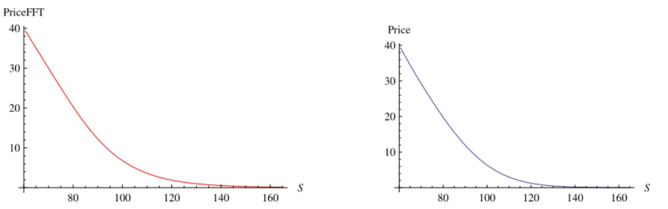
Figure 3.3: Left: The price of an European put option using Fast Fourier Transform. Right: The price of an European put option using the finite difference scheme.

60 80 100 120 140 160

x

0.002 0.004 0.006 0.008 0.010 0.012 0.014

Error

0.0 0.2 0.4 0.6 0.8 1.0

Τ

0.02 0.04 0.06 0.08 0.10

Error

Figure 3.4: Left: The error metric in % as a function of x ,when τ =T. Right: The error in % as a function of τ, when x= 0.

3.3.3.1 Numerical Results

In this section we briefly present a numerical experiment using the finite difference scheme described above and compare it with the widely known Fast Fourier transform method that can be used in this case for option pricing because the characteristic function of the Variance Gamma process is known analytically. The process considered was the Variance Gamma with

θ = ₋0.33, σ = 0.12, κ = 0.16, r = 0,∆x = 0.01,∆t = 0.005, K = 100, A = 1, ǫ = 0.6, T = 1 for the case of an European put option. The price as a function of the underlying for the two methods is shown in Figure (3.3). We see that the function that represents the European put option price using the finite difference scheme is very similar to the price of an European put option using the Fast Fourier Transform. The error between the two methods for two cases is displayed in Figure (3.4) and as we can see is relatively small. In order to compare the two methods the error metric used (as in [CV05a]) was the difference in absolute value between the implied volatilities under the two methods:

(32)

Chapter 4

Option prices as viscosity solutions

of PIDEs

In this chapter we introduce the notion of viscosity solution in the PIDEs frame, that was first introduced by Crandall and Lions ([CL92]). We saw in Section 3.1 that if some conditions of smoothness are satisfied, then the option price function is a classical solution of the associated partial integro-differential equation. But, as we saw in the examples of pure jump processes in Section 3.2, the option price functions were not smooth. This motivates us to consider the notion of viscosity solution. As we will see in Section 4.2, if we consider more general conditions, we can express option prices , such as barrier or European options, as viscosity solutions of certain PIDEs. In this introduction we give an idea of such concept. Consider a regular solution f of the equation:

∂f

∂τ −Lf −r ∂f

∂x = 0 (4.1)

where Lf is given by (2.10).

Then, ifϕis a regular function such thatf ₋ϕhas a global maximum at (τ, x), we have:

∂ϕ

∂τ −Lϕ−r ∂ϕ

∂x ≤0 (4.2)

In fact, because (τ, x) is a global maximum, we have:

∂(f ₋ϕ)

∂τ (τ, x) =

∂(f₋ϕ)

∂x (τ, x) = 0, (4.3)

∂2(f−ϕ)

∂x2 (τ, x)≤0. (4.4)

and also _∀(τ, y),

f(τ, x)₋ϕ(τ, x)_≥f(τ, y)₋ϕ(τ, y)_⇔f(τ, y)₋f(τ, x)_≤ϕ(τ, y)₋ϕ(τ, x). (4.5)

(33)

4.1. Definitions 27

Then,

0 = ∂f

∂τ −Lf−r ∂f

∂x (4.6)

= ∂f

∂τ − σ2

2

∂2f ∂x2 +

σ2

2 −r

∂f

∂x(τ, x)−

Z

R

[f(τ, x+y)₋f(τ, x)₋(ey₋1)∂f

∂x]ν( dy)(4.7)

≥ ∂ϕ

∂τ − σ2

2

∂2ϕ ∂x2 +

σ2

2 −r

∂ϕ ∂x −

Z

R

[ϕ(τ, x+y)−ϕ(τ, x)−(ey −1)∂ϕ

∂x]ν( dy) (4.8)

= ∂ϕ

∂x. (4.9)

On the other hand if ϕis a regular function and (τ, x) is a globlal minimum of f₋ϕwe have

∂ϕ

∂x ≥0. (4.10)

We are going to see that iff satisfies (4.9) and (4.10), thenf is called a viscosity solution, which is nothing but a generalization of solution. This wayf doesn’t need to belong to C1,2. Iff is a viscosity solution and also a function of classC1,2_{, then}_f _{is also a solution in the classical sense.}

In fact, we could set ϕ=f, then f −ϕ= 0 and all (τ, x) is a global minimum and maximum. Then by (4.9) and (4.10) we have:

∂f

∂τ −Lf −r ∂f ∂x =

∂ϕ

∂x = 0. (4.11)

4.1 Definitions

Consider the following definitions that we will need to formalize the concept of viscosity solution. Let

U SC=_{v: [0, T)_×R_→R: v is an upper semicontinuous function _}, (4.12)

and

LSC={v: [0, T)×R_→R: v is a lower semicontinuous function }. (4.13)

Also,

M=_{φ:φ is a measurable function_}

C_p+([0, T]_×R) =_{φ:φ_{∈ M} and _∃C >0,_|φ(t, x)_{| ≤}C(1 +_|x_|p1x>0)}.

This way, Lϕcan be defined for ϕ_∈C+

(34)

28 Chapter 4. Option prices as viscosity solutions of PIDEs

Lϕ(x) =γ∂f ∂x+

σ2

2

∂2_f

∂x2 +

Z

|y|≤1

ν( dy)[ϕ(x+y)₋ϕ(x)₋y∂ϕ ∂x(x)]

+

Z

|y|>1

ν( dy)[ϕ(x+y)−ϕ(x)]. (4.14)

The terms in (4.14) are well defined because forϕ∈C2([0, T]×R):

|ϕ(τ, x+y)−ϕ(τ, x)−y∂ϕ

∂x(τ, x)| ≤y

2 _sup

|x|≤1|

ϕ′′(τ, .)|for |y| ≤1. (4.15)

and for ϕ_∈C+

p([0, T]×R) : _Z y>1

ypν( dy)<∞. (4.16)

Let O= (a, b)_⊆Rbe an open interval, ∂O=_{a, b_} the boundary ofO. Consider the following initial boundary value problem on [0, T]×R:

∂f

∂τ =Lf+r ∂f

∂x,(0, T]×O, (4.17) f(0, x) =h(x), x_∈O; (4.18)

f(τ, x) =g(τ, x), x /∈O (4.19) We now present the definition of viscosity solution:

Definition 4.1.1 A function v _∈ U SC is a viscosity subsolution of (4.17)₋(4.19) if _∀ϕ _∈ C2_([0_{, T}_]_×_R₎_∩_C+

p ([0, T]×R) and for all global maximum point (τ, x)∈[0, T]×Rof v−ϕthe

following properties are verified:

∂ϕ

∂x ≤0, if(τ, x)∈(0, T]×O (4.20)

min

∂ϕ

∂x, v(τ, x)−h(x)

≤0, if τ = 0, x_∈O, (4.21)

min

∂ϕ

∂x, v(τ, x)−g(τ, x)

≤0, if τ _∈(0, T], x_∈∂O, (4.22)

v(τ, x)≤g(τ, x), if x /∈O (4.23)

A function v _∈ LSC is a viscosity supersolution of (4.17)₋(4.19) if _∀ϕ_∈ C2([0, T]_×R)_∩

C+

p ([0, T]×R)and for all global minimum point(τ, x)∈[0, T]×Rofv−ϕthe following properties

are verified:

∂ϕ

∂x ≥0, if(τ, x)∈(0, T]×O (4.24)

max

∂ϕ

∂x, v(τ, x)−h(x)

≥0, if τ = 0, x_∈O, (4.25)

max

_∂ϕ

∂x, v(τ, x)−g(τ, x)

≥0, if τ _∈(0, T], x_∈∂O, (4.26)

v(τ, x)_≥g(τ, x), if x /_∈O (4.27)

A function v_∈C_p+([0, T]_×R) is called a viscosity solution of (4.17)₋(4.19) if it is simulta-neously a subsolution and a supersolution. Then v is continuous on (0, T]_×R.

(35)

4.2. Option prices as viscosity solutions of PIDEs 29

4.2 Option prices as viscosity solutions of PIDEs

The main tool for showing uniqueness of viscosity solutions is the comparison principle presented in [Vol05].

Proposition 4.2.1 Let u _∈U SC and v _∈ LSC with polynomial growth. If u is a subsolution and v is a supersolution of (4.17)−(4.19) with O =R and the function h is continuous, then

u_≤v on[0, T]_×R.

The following proposition indicates that the values of European and barrier options in a exponential L´evy model can be expressed as the viscosity solutions of (4.17)−(4.19).

Proposition 4.2.2 Let the payoff function H verify the lipschitz condition (3.17)and leth(x) =

H(S0ex) verify the condition of polynomial growth at infinity:

|h(x)_{| ≤}C(1 +_|x_|p1x>0). (4.28)

Then:

1) The forward valuefe(τ, x) of an European option defined by f(τ, x) =E[h(x+rτ +Xτ)]

is a viscosity solution of the Cauchy problem (4.17)−(4.19) withO =R.

2) The forward valuefb(τ, x) of a knockout barrier option defined by (3.37),(3.39)or (3.41)

is a viscosity solution of the Cauchy problem (4.17)₋(4.19) withg= 0.

M ESTRADO M ATEMÁTICAF

M

ESTRADO

M

ATEMÁTICA

F

INANCEIRA

T

RABALHO

F

INAL DE

M

ESTRADO

DISSERTAÇÃO

INTEGRO-DIFFERENTIAL EQUATIONS FOR OPTION

PRICING IN EXPONENTIAL LÉVY MODELS

JOSÉ MANUEL TEIXEIRA DOS SANTOS CRUZ

M

ESTRADO EM

M

ATEMÁTICA

F

INANCEIRA

T

RABALHO

F

INAL DE

M

ESTRADO

DISSERTAÇÃO

INTEGRO-DIFFERENTIAL EQUATIONS FOR OPTION

PRICING IN EXPONENTIAL LÉVY MODELS

JOSÉ MANUEL TEIXEIRA DOS SANTOS CRUZ

O

RIENTAÇÃO

:

JOÃO

MIGUEL

ESPIGUINHA

GUERRA

Acknowledgements

Contents

Chapter 1

Introduction

Chapter 2

Financial Modelling with L´

evy

Processes

2.1

L´

evy Process: definitions

2.2

Exponential L´

evy models

2.3

Examples of L´

evy processes in finance

Chapter 3

Integro-differential equations for

option pricing

3.1

Definitions

3.2

Feynman-Kaˇ

c formula for PIDEs

3.3

Option prices as classical solutions of PIDEs

Chapter 4

Option prices as viscosity solutions

of PIDEs

4.1

Definitions

4.2

Option prices as viscosity solutions of PIDEs