M
ASTER
F
INAL
W
ORK
CAPITAL STRUCTURE AND DIVIDENDS
Evidence from Portugal (2003-2014)
A
NA
M
ARGARIDA
S
ANTOS
S
IMÕES
F
ERREIRA
2
MASTER
F
INANCE
M
ASTER
F
INAL
W
ORK
CAPITAL STRUCTURE AND DIVIDENDS
Evidence from Portugal (2003-2014)
A
NA
M
ARGARIDA DOS
S
ANTOS
S
IMÕES
F
ERREIRA
S
UPERVISOR:
PROF. JOAQUIM MIRANDA SARMENTO
3
Index
List of Equations………. 5
List of Tables………... 6
Acknowledgements……… 7
Abstract……… 8
Introduction……….. 9
1. Literature review 11 1.1 Trade-Off ... 12
1.2 Pecking Order ... 16
2. Methodology 19 2.1 Sample and analysed period ... 19
2.2 Definition of variables ... 19
2.3 Descriptive statistics ... 24
2.4 Regressions ... 24
2.4.1 The first Testing Hypothesis ... 24
2.4.2 The second Testing Hypothesis ... 26
2.4.3 The third Testing Hypothesis ... 28
3. Results 30 3.1 First Testing Hypothesis ... 30
3.1.1 The relationship between Dividends and Investment: RDtAt ... 30
3.1.2 The relationship between Dividends and Profitability Et/At; Vt/At ... 31
3.1.3 The relationship between Dividends and Volatility: ln(At) ... 32
3.2 Second Testing Hypothesis ... 32
3.3 Third Testing Hypothesis ... 34
4
3.3.2 The relationship between Leverage and Investment Opportunities RD/At (5), RDDt(4) .. 36
3.3.3 The relationship between Leverage and Volatility ln(At) (6) ... 36
3.3.4 The relationship between Leverage and Non-Debt Tax Shield RDt/At (5) DP/At (3) ... 37
4. Conclusions 38
5
List of Equations
Equation (1) ... 25
Equation (2) ... 25
Equation (3) ... 25
Equation (4) ... 26
Equation (5) ... 26
Equation (6) ... 26
Equation (7) ... 27
Equation (8) ... 27
Equation (9) ... 28
Equation (10) ... 28
Equation (11) ... 28
6
List of Tables
Table I - Population of the study - list of Companies. ... 44
Table II - Pecking Order vs Trade-Off Predictions ... 45
Table III - Variables Description ... 47
Table IV - Proxies ... 48
Table V - Ratios ... 49
Table VI - Descriptive statistics ... 50
Table VII - Fama and French (2002) Regressions used to understand how Target Pay-Outs behave when they are a function of investment opportunities, profitability and volatility proxies. ... 51
Table VIII - Lintner model regression to explain variations in Dividend Targets ... 53
7
Acknowledgements
At this academic stage in which I am finishing the Master in Finance, I would like to express through these words, my most sincere gratitude for those who had contributed both directly and indirectly to my accomplishment. To all of those, I give my truthful thank you.
I would also like to cement my deep gratefulness towards my professor Joaquim Miranda Sarmento, for all the support and time spent on the most difficult moments, who helped me to turn my doubts into knowledge. Once again I am grateful to professor Joaquim Miranda Sarmento, especially for the hours of dedication in which his professionalism and scientific rigor were decisive to the deepening and enrichment of this work.
To my family, in particular to my parents and sister for the opportunities they had provide me in my entire life.
8
Abstract
We use the Portuguese case to replicate the study of Fama & French (2002) regarding the capital structure and the connections between profitability, investments and volatility with dividends pay-out and leverage. Our aim is to analyse the relation between capital structure, dividends and interests on equity, using the Portuguese companies traded on Euronext, for the period between 2003 and 2014.
In this research we found evidence supporting that Portuguese companies share the predictions of Pecking Order and Trade-Off models. In some cases, the predictions are the same, and differ only regarding the motive, which is the case of: (1) profitability and dividends; (2) dividends and investments; (3) volatility and dividends. When the models’ predictions are set differently, the main goal is to identify whether it behaves, or does not behave according to Pecking Order or Trade Off. For instance, Portuguese companies behave according to the Pecking Order model with regards to the relationship between leverage and profitability. There are also situations where it is necessary to observe beyond the simple model, i.e., to the complex pecking order model , in order to understand what happens to companies’ leverage with changes in investment opportunities. One of the others main conclusion is that the target dividends do not absorb short term variations of investment, as the Speed of Adjustment is not big enough to accomplish a total sort term variation
9
Introduction
10
based on Pecking Order vs. Trade-Off. This particular study relies on testing how leverage and dividends pay-out react with changes in investment opportunities and profits in Portuguese companies. In order to understand these issues, this research is divided into three different testing hypotheses. The first hypothesis that is tested is whether the target of dividend pay-out ratio changes with: (1) investment; (2) profitability, and; (3) volatility. Secondly, whether target dividend pay-outs are adjusted to absorb short term variation of investments is tested. The next hypothesis is related to the leverage of companies. In this specific case, the aim is to understand whether Portuguese companies behave in line with the Pecking Order, or Trade Off predictions, i.e., by relating leverage with: (1) profitability; (2) investments opportunities; (3) volatility, and; (4) non debt tax shield.
As a result of all of these testing hypotheses, it is possible, in a very superficial way, to identify some of the share predictions that are present in the literature with Portuguese companies. As an example, our predictions are in accordance with Fama and French (2002), examples being profitability and dividends and volatility and dividends.
An interesting conclusion of this study concerns dividends and investments; where evidence was founded suggesting that shareholders are probably so levered, that they need dividends, even when this goes against the company’s interest.
Evidence was also found that dividend pay-outs are not used to absorb short term variations in investment, as the speed of adjustment is lower than 1.
11
1. Literature review
Modigliani&Miller (1958) developed a theory which states that in perfect capital markets, the composition of capital is irrelevant when they want to finance investments. They explain that it is the possibility that earnings and the risk of their underlying assets that define their market value, in other words, it is indifferent which method is chosen to finance their investments or dividends pay-out. However this theory is supported by strong assumptions of no taxes, no transaction costs, no bankruptcy costs, and that the cost of debt is the same for companies and investors alike, with no asymmetric information, and finally, that the EBIT1 is unaffected by the debt. In a simple view, this proposition is transmitted by a constant WACC2, even with variations in the capital structure. Maybe this example would be easier to understand in the case of a company that does not benefit from tax advantages by interest payments, and that the way that the firm financed itself is equal. Furthermore, when there are no variations or advantages from rising debt, a company's stock price remains the same.
Nevertheless, we must take care that in the real world there are taxes and bankruptcy costs, and these affect a company's stock price, and that the MM theorem apply. That is why they included the effect of taxes and bankruptcy costs. When submitted according to Modigliani and Miller'sTrade-Off Theory of Leverage, this model takes these two variables into account. This model explains the benefits of leverage on capital structure, until the optimal capital structure3 is attained. Controversy surrounds this example, now that a tax benefit from interest payments is identified.
1 Earnings Before Interest and Taxes 2 Weighted Average Cost of Capital
3The optimal capital structure is when a firm attains the best debt to equity ratio and increases it to a
12 1.1 Trade-Off
The Trade-Off theory is based on the concept of a company maximizing its value by reaching an equilibrium between the costs and benefits of an additional unit of debt. The same idea is used for dividends, where a company establishes a level dividend pay-out whereby the company maximizes its value. Before looking at the Trade-Off model in detail view, we must start inquiring as to why companies pay dividends.
13
1981). The act of contracting an audit company allows for the examination of a firm, and enables proof about the behaviour of the managers, including whether they have been truthful and whether what they transmit to the investors is the real scenario of the company.
14
accomplished once a year, instead of quarterly, and that investors are then attracted to a long run of capital gains, which would be capable of trading shares earlier to escape the ex-day, and consequently by the tax payments on the dividends. This strategy allows a reduction of administrative and transaction costs. Finally, the authors mention that which has already been stated, that managers should seek other less expensive ways of transmitting credibility.
Easterbrook (1984) follows other path, which mentions that dividends keep firms in capital markets, and that for this reason, it is possible to control managers with lower costs. Dividends are also used to influence financing polices, and this might be a valid reason for why firms use this outflow of cash and raise funds (issue stock, or new debt) at the same time.
15
Regarding the relation of taxes and leverage, it is quite important to take a detailed look at what DeAngelo & Masulis (1980) presented. They carried out an extension of Miller, changing the existent model, as it was too sensitive with regards to changes of corporate tax policies. According to DeAngelo & Masulis (1980), there is a non-debt tax shield 4that should be included, such as depreciation and investment tax credit, which should be included in the model. In short, this new model requires more than one debt tax shield to attain an optimal level of leverage. Regarding this research, equilibrium of leverage is exclusive for each company, so it is important to include variables such as were mentioned beforehand, in order to define this. It is also stated that personal and corporate taxes are present in relative market prices. Another important component are bankruptcy costs, which must be considered if we want to extract the tax benefit that is related to leverage cost. One of the predictions of this model is that firms have debt-level that has a negative relation with the non-debt tax shield. The authors also mentioned that modifications in debt bring variations to a company’s valuation. Therefore, in a situation of equilibrium, relative market prices will involve the tax advantage for corporate debt financing. Should fiscal changes exist (reducing their amount) regarding policies related to non-debt tax shield, then this will be reflected by increases in the amount of debt that firms purchase. Finally, DeAngelo & Masulis (1980) explain that bankruptcy costs are negatively correlated to debt. This idea is also consistent with Brandley, Jarrel & Kim (1984), as they stated that the expected cost of financial necessities and the amount of non-debt tax shield are negatively related to the optimal level of leverage. It is also pointed out that in a situation where the costs of financial distress are non-trivial, changes in firms’ earnings and volatility will negatively influence the level of leverage. Another
4 Non debt tax shield is a reduction in the taxable amount of a company, by applying deductions on
16
component which interferes with leverage in a negative way, is the intensity of R&D and publicity expenditure. Authors have also pronounced that a kind of perplexity exists, which finds a direct relation between firms’ leverage and the comparative amount of non-debt tax shields. However, this goes against the previous literature, which defends the replacement of non-debt tax shield for debt tax shields.5 A possible explanation referred to by the authors, is that a non-debt tax shield has more influence on the openness of firms’ assets, as it infers safety assets and rising leverage ratios.
With regards to taxes and the Trade-Off model, it is necessary to point out another relevant study, that of Miller & Scholes (1978). In this study, it was proved that shareholders’ welfare is also affected by the increase or decrease in dividends, independent of the discrepancy of the tax treatment on capital gains and dividends. With regards to debt level and company size, there are some studies which are consistent with most of the existing theories, for example, that of Titman & Wessels (1988). One of the founded evidences on that study, is that debt level is inversely related to the size of the company. Small firms tend to have higher short-term debt and lower long-term debt ratios. They also suggested that this might be a consequence of the high cost that small companies face when they try to issue long-term financial instruments.
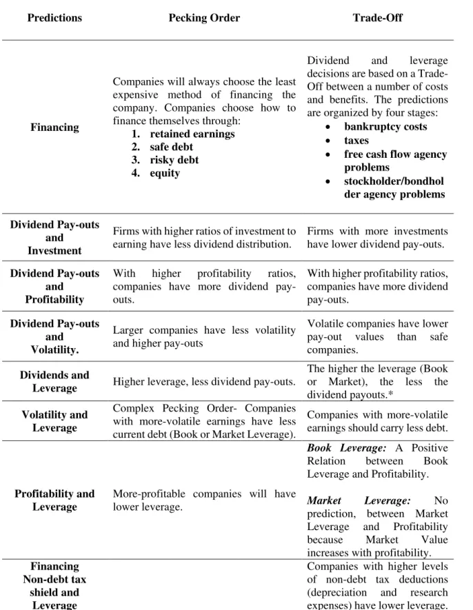
Table II (Appendix - page 45) illustrates Trade-Off predictions.
1.2 Pecking Order
In order to explain the Pecking Order model, the study of Myers & Majluf,(1984) needs to be observed first. In this research, one of the big issues of these authors was how investment opportunities should be financed, as managers are the ones who possess more information (even more than shareholders). The other big question raised is whether it
5Debt tax shield is a reduction in the taxable amount of a company, by applying deductions through debt
17
might be preferable to pass up investment opportunities or the issuing of stock, when a company needs to be financed.
According to the Myers (1984) model, managers possess better information in comparison to investors. Therefore, the main conclusion of this model is that for the company it is always better to start with risk-free debt, by issuing safer securities than risk. If a company needs to obtain external capital, then it should resort to bonds market, and if it want to increase equity, then it should do so by retention.
According to Myers, situations may exist whereby it is preferable to renounce good investments, rather than issue risky securities in order to finance them. Or, for instance, firms may even accumulate financial slack, and they can do this by restricting the amount of dividend pay-outs, by saving assets that are easily sold, preserving borrowing power and simply by saving cash. Myers goes even further, by explaining that companies ought not to pay dividends if they need to recover cash by selling stocks or other securities risk. The author also explains that dividends are a tool for communicating with the market, and that dividends are high correlated with managers estimating the value of asset. Finally, it has been suggested in this study that, if stocks are issued to finance investments and managers have more information, then the price will fall. On the other hand, if companies issue safe default risk free debt to finance investment, then the stock price will not decrease. In conclusion, what is possible to extract is that internal funds are preferable to external funds.
18
dividend payment, Fama and French divided companies into three different groups: Ex-Payer; Never Paid, and; Dividend Payers. The first conclusion is that Ex-Payers have the lowest earnings and the lowest values of investment. Secondly, companies that Never Paid dividends are more profitable than the former payers, with a higher opportunity for growth. This group is the one that has greater investment and a higher ratio of Market value of Assets to their book value. Finally, Dividend Payers are the most profitable. Another suggestion raised in this study, is that, included amongst those that pay dividends, are those that have higher ratios, which tend to be larger and more profitable. On the other hand, small companies with higher values of investments have lower ratios of dividends. This behaviour is consistent with a reluctance for risk security, on account of the existence of asymmetric information problems or transaction costs.
19
2. Methodology
2.1 Sample and analysed period
The data was extracted from Bloomberg6, and is composed of Portuguese companies (see the detailed list in Appendix page 44 –Table I) which are traded on Euronext and have information available for the period of 2003 to 2014.
2.2 Definition of variables
Some of the variables need to be transformed. For volatility, investment opportunities and profitability proxies were carried out by an extension of Fama & French’s (2002) procedures.
As for representation for profitability, three different indicators are used: (1) Earnings before Interest and Taxes, divided by the Total Assets; (2) Earnings before Interest, also divided by Total Assets; (3) Market Value of the firm, (which is represented by liabilities minus deferred taxes, and investment tax credit, plus preferred stocks, and plus market equity), divided by Total Assets, which characterises profitability and investment opportunities simultaneously. Investment opportunities is also represented by: (4) Variations in Assets, divided by Total Assets, and; (5) Research and Development also, divided by Assets.
The proxy used for volatility is: (6) the Logarithm of the Assets, which is the size, representing the (inverse) probability of default. Finally, the representation of applied non-debt tax shield7 is: (7) Research and Development, and; (8) Depreciation Expense, both divided by Assets.
20
Due to the complexity of both variables and ratios, the following paragraphs show, step by step, their construction. It is also possible to observe them in a simpler manner in Table III, Table IV and Table V (Appendix - pages 47, 48 and 49).
Table III presents the simple variables, i.e., items taken from the financial records, or a slightly altered variable.
• At represents Total Assets at moment t, and At1 Total Assets at moment t+1;
• dAt is the variation in Total Assets at moment t;
• LN (At) is the ln of the Asset at moment t;
• D is the variable which represents the value of Dividends;
• Et is the Earnings before Interest for moment t, created by the subtraction of Tax
Expenses on Earnings before interest and expenses, and Et1 at the same moment as t+1;
• ETt is the Earnings before Interest and Taxes, which is constructed by the
EBITDA, adding depreciation and amortization at moment t;
• dEt is the variation, which is Earnings before Interest at moment t, minus its value
at t-1;
• dETt is the change in Earnings before Interest and Taxes of t and t-1;
• Met is Market Equity, which is the number of shares, multiplied by the number of
shares at moment t;
• Vt is the Market Value of the firm, at moment t, constructed by the subtraction of
Deferred Taxes and Investments Tax Credit on Liabilities, followed by the addition of Preferred Stocks and Market Equity;
21
• RDDt is a dummy variable, which takes the value 0, if there are R & D
Expenditures, and the value of 1 otherwise;
• Dt, which represents the value of Depreciation Expenses at moment t;
• Lt is the Liabilities, which is the sum of Short and Long Term Debt;
• NSt is the number of Shares Outstanding at moment t;
• SPt represents Stock Price at moment t;
• Dst is the Variation of The Stock Price, which is represented by;
• Yt is the Variations of Market Capitalisation, which is the variation between
moment t and t-1 of the Number of Shares, multiplied by the Stock Price;
• BE is Book Equity, which is Total Assets minus Liabilities, plus Deferred Taxes
and Investment Tax Credits, minus Preferred Stock.
Table IV (Appendix - page 48) and Table V (Appendix - page 49) are the build ratios
from a better short view, and the next paragraph shows their computation in a more detailed way:
• ETtAt consists of the Division of Earnings before Interest and Taxes at moment t
for Total Assets, at the same moment;
• Et/At is Earnings before Interest at moment t, divided by Total Assets at moment
t;
• VtAt represents the Market Value of the Firm at moment t, divided by Total Assets
at moment t;
• dAtAt is the variable used to represent the Ratio of Variation of Total Assets
between t-1, and t for the Total Assets at moment t;
• RDtAt is the Division of R & D Expenditures at moment t by the Total Value Of
22
• DPtAt is the ratio that relates Depreciation Expenses with Total Assets at moment
t;
• LtVt represents the liabilities at moment t, divided by the Market Value of The
Firm at moment t;
• LtAt is Liabilities divided by Total assets. LAL is the variable applied to show the
variations of Liability ratios to Total Assets of t+1 to t;
• Dt1At1 represents the division of Dividends to Assets, both at moment t+1;
• YA is the Variation of Market Capitalisation t+1, divided by Total Assets t;
• Yt1At1 represents the ratio at moment t+1 of Stock Earnings to Total Assets;
• DDA is the Variation of Dividend at moment t+1 to moment t, divided by Total
Assets at moment t;
• DA is the value of Dividends at moment t, divided by Total Assets for the next
period;
• dAA is composed by the Difference of Assets between t and t+1, divided by Total
Assets at moment t+1;
• BL is the division of Liabilities at moment t+1 by the Total Assets in the same
period;
• ML is Market Leverage at moment t+1, which is Liabilities at t+1, divided by the
Market Value of the Firm at moment t; • Det is the Change of EBI for moment t+1;
• DEA is the Change of EBI for moment t+1, divided by Total Assets at moment
t+1;
• DAA is the Variation of Total Assets between t and t-1, divided by Total Assets at
23
24 2.3 Descriptive statistics
305 observations exist for all variables and for all of them the mean is positive with the exception of dSPt, the Variation of Stock Price, and Yt, the Variation of Market Capitalisation at moment t.
Some of the variables used for this study have negative minimum values, such as, D; Et;
dEt; ETt; dETt; Q; BE; Dst;Yt; ETtAt; EtAt; dAtAt: Dt1; Yt1; Et1. Others have a
minimum of zero, such as Met; RDt; RDDt; DPt; NSt; SPt; RDtAt and DPtAt. At, Vt, Lt,
LNAt, VtAt, LtVt,LtAt, Lt1, Vt1, At1 took positive minimums. In fact, all of the variables have at least one positive value once the maximum values are all positive. A value of 1 exists, on account of the variable being a RDDt dummy. The descriptive statistics can be observed in Table VI (Appendix - page 50).
These variables have passed the test of multicollinearity heteroscedasticity, through the Matrix of correlation, and the Breusch-Pagan and Wald tests. The regressions used and the test made were performed by Stata.8
2.4 Regressions
2.4.1 The first Testing Hypothesis
In this first testing hypothesis, the main objective of this study is to understand how dividends target pay-out changes with variations in profitability, investment opportunities, and leverage. Previous studies, such as that of Lintner (1956), have a model that explains how dividends behave, however, only for dividends as a function of the target pay-out (r), the current value after taxes profit ( Pit), and the last amount of dividends paid (Di(t-1), as shown in Equation 1.
25
Equation (1)
𝐷𝐷𝑖𝑖𝑖𝑖 =𝑎𝑎𝑖𝑖 +𝑐𝑐𝑐𝑐𝑐𝑐𝑖𝑖𝑖𝑖+ (1− 𝑐𝑐)𝐷𝐷𝑖𝑖(𝑖𝑖−1)+𝑢𝑢𝑖𝑖𝑖𝑖
In Lintner (1956), p.14 – 109
For this reason, and since the aim is to understand how dividends react when they are a function of profitability, investment opportunities and leverage, one should follow Fama & French (2002), who developed another regression where the coefficient of the net profit is affected by other variables.
Equation (2)
𝐷𝐷𝑖𝑖+1⁄𝐴𝐴𝑖𝑖+1=𝑎𝑎0+ (𝑎𝑎1+𝑎𝑎1𝑉𝑉𝑉𝑉𝑖𝑖⁄𝐴𝐴𝑖𝑖+𝑎𝑎1𝐸𝐸𝐸𝐸𝑖𝑖⁄𝐴𝐴𝑖𝑖+𝑎𝑎1𝐷𝐷𝑅𝑅𝐷𝐷𝐷𝐷𝑖𝑖+ 𝑎𝑎1𝑅𝑅𝑅𝑅𝐷𝐷𝑖𝑖⁄𝐴𝐴𝑖𝑖 +𝑎𝑎1𝑆𝑆𝑙𝑙𝑙𝑙(𝐴𝐴𝑖𝑖) +𝑎𝑎1𝐿𝐿𝑇𝑇𝑇𝑇𝑖𝑖+1+ 𝑎𝑎1𝐴𝐴𝑑𝑑𝐴𝐴𝑖𝑖⁄𝐴𝐴𝑖𝑖) × 𝑌𝑌𝑖𝑖+1⁄𝐴𝐴𝑖𝑖+1+ 𝑒𝑒𝑖𝑖+1
In Fama & French (2002), p.10
In Equation (2), it is possible to observe that the target pay-out and the consequences of the dividends are explained by profitability volatility and non-debt tax shield investment opportunities. The regression used in this study is slightly different from that of Fama & French (2002), which finally excludes the variable that would have the multiplication of all estimated coefficient and the explanatory variables model as its coefficient. The regressions used for this test are the following:
• Target book leverage
Equation (3)
26 • Target market leverage
Equation (4)
𝐷𝐷𝑖𝑖+1⁄𝐴𝐴𝑖𝑖+1=𝑎𝑎0+ 𝑎𝑎1𝑉𝑉𝑖𝑖⁄𝐴𝐴𝑖𝑖+𝑎𝑎2𝐸𝐸𝑖𝑖⁄𝐴𝐴𝑖𝑖+𝑎𝑎3𝑅𝑅𝐷𝐷𝐷𝐷𝑖𝑖+ 𝑎𝑎4𝑅𝑅𝐷𝐷𝑖𝑖⁄𝐴𝐴𝑖𝑖 +𝑎𝑎5𝑙𝑙𝑙𝑙(𝐴𝐴𝑖𝑖) +𝑎𝑎6𝑑𝑑𝐴𝐴𝑖𝑖⁄𝐴𝐴𝑖𝑖+ 𝑎𝑎7𝑇𝑇𝑖𝑖⁄𝑉𝑉𝑖𝑖+ 𝑒𝑒𝑖𝑖+1
2.4.2 The second Testing Hypothesis
At this point, the goal of this research is to understand whether the dividend pay-outs are adjusted to absorb short term variations in investments. Therefore, in order to have a regression that includes changes in dividends because variations around the target pay-out make sense to return to Lintner’s (1956) adjusted model, shown in Equation (5). However, for the same reasons that were presented in Fama & French (2002), the impossibility of relating dividends with investments is shown in the equation, which turns out to be misleading in explaining the speed of adjustment to targets pay-out, taking into consideration that which we wish to understand.
Equation (5)
𝐷𝐷𝑖𝑖+1− 𝐷𝐷𝑖𝑖 =𝑎𝑎1𝑌𝑌𝑖𝑖+1+𝑎𝑎2𝐷𝐷𝑖𝑖+𝑒𝑒𝑖𝑖+1
In Fama &French (2002), p.10
For this reason, and in order to measure the speed of the adjustment of dividends to the supply of short term investment variations presented, such as in Fama & French (2002), as shown in Equation (6), which is a model created by Fama & MacBeth (1973).
Equation (6)
27
In Fama & French (2002), p.15
Equation (6) is one step ahead of Lintner (1956), as it allows for the average variation during the years, instead of only taking into consideration the normal variations of dividends to the target pay-out. However, according to Fama & French (2002), the targets of distribution and the speed are different for each company, and that is why they presented equation (7).
Equation (7)
(𝐷𝐷𝑖𝑖+1− 𝐷𝐷𝑖𝑖)⁄𝐴𝐴𝑖𝑖+1
=𝑎𝑎0 + (𝑎𝑎1𝑉𝑉𝑉𝑉𝑖𝑖⁄𝐴𝐴𝑖𝑖+𝑎𝑎1𝐸𝐸𝐸𝐸𝑖𝑖⁄𝐴𝐴𝑖𝑖+𝑎𝑎1𝐴𝐴𝑑𝑑 𝐴𝐴𝑖𝑖⁄𝐴𝐴𝑖𝑖+𝑎𝑎1𝐷𝐷𝑅𝑅𝐷𝐷𝐷𝐷𝑖𝑖 +𝑎𝑎1𝑅𝑅𝑅𝑅𝐷𝐷𝑖𝑖⁄𝐴𝐴𝑖𝑖+𝑎𝑎1𝑆𝑆𝑇𝑇𝑙𝑙(𝐴𝐴𝑖𝑖) +𝑎𝑎1𝐿𝐿𝑇𝑇𝑇𝑇𝑖𝑖+1) ×𝑌𝑌𝑖𝑖+1⁄𝐴𝐴𝑖𝑖+1 + (𝑎𝑎2+𝑎𝑎2𝑉𝑉𝑉𝑉𝑖𝑖⁄𝐴𝐴𝑖𝑖+𝑎𝑎2𝐸𝐸𝐸𝐸𝑖𝑖⁄𝐴𝐴𝑖𝑖+𝑎𝑎2𝐴𝐴𝑑𝑑 𝐴𝐴𝑖𝑖⁄𝐴𝐴𝑖𝑖+𝑎𝑎2𝐷𝐷𝑅𝑅𝐷𝐷𝐷𝐷𝑖𝑖
+𝑎𝑎2𝑅𝑅𝑅𝑅𝐷𝐷𝑖𝑖⁄𝐴𝐴𝑖𝑖+𝑎𝑎2𝑆𝑆𝑇𝑇𝑙𝑙(𝐴𝐴𝑖𝑖) +𝑎𝑎2𝐿𝐿𝑇𝑇𝑇𝑇𝑖𝑖+1) ×𝐷𝐷𝑖𝑖⁄𝐴𝐴𝑖𝑖+1+𝑏𝑏1𝑑𝑑 𝐴𝐴𝑖𝑖+1⁄𝐴𝐴𝑖𝑖+1 +𝑒𝑒𝑖𝑖+1
In Fama &French (2002), p.16
Due to the lack of data in this research, only two variations of the equation (6) were used, instead of equation (7). Therefore the equations applied in this study are the following:
• Market leverage
Equation (8)
(𝐷𝐷𝑖𝑖+1− 𝐷𝐷𝑖𝑖)⁄𝐴𝐴𝑖𝑖+1
28 • Book leverage
Equation (9)
(𝐷𝐷𝑖𝑖+1− 𝐷𝐷𝑖𝑖)⁄𝐴𝐴𝑖𝑖+1
=𝑎𝑎0+𝑎𝑎1𝑌𝑌𝑖𝑖+1⁄𝐴𝐴𝑖𝑖+1+𝑎𝑎2𝐷𝐷𝑖𝑖⁄𝐴𝐴𝑖𝑖+1+𝑎𝑎3𝑑𝑑 𝐴𝐴𝑖𝑖+1⁄𝐴𝐴𝑖𝑖+1 +𝑎𝑎4𝑇𝑇𝑖𝑖⁄𝐴𝐴𝑖𝑖+𝑒𝑒𝑖𝑖+1
2.4.3 The third Testing Hypothesis
At this phase of the research, the focus is to understand the behaviour of leverage. In order to achieve this goal, similar regression to that of Fama & French (2002) is used. This regression relates Book and Market leverage, as both are a function of investment opportunities, profitability and volatility proxies. Using a regression with these variables, it is possible to understand whether companies in Portugal are more likely to behave according to the Pecking Order or the Trade-Off model, as profitability and investment opportunities proxies are used. With these tests it is also possible to observe whether companies use debt to absorb short term variations of earnings and investments. In order to construct the final regression, Equation 10 was used (Fama & French, 2002).
Equation (10)
𝑇𝑇𝑖𝑖+1⁄𝐴𝐴𝑖𝑖+1 =𝑏𝑏0+𝑏𝑏1𝑉𝑉𝑖𝑖⁄𝐴𝐴𝑖𝑖+𝑏𝑏2𝐸𝐸𝑇𝑇𝑖𝑖⁄𝐴𝐴𝑖𝑖+𝑏𝑏3𝐷𝐷𝐷𝐷𝑖𝑖⁄𝐴𝐴𝑖𝑖+𝑏𝑏4𝑅𝑅𝐷𝐷𝐷𝐷𝑖𝑖+𝑏𝑏5𝑅𝑅𝐷𝐷𝑖𝑖⁄𝐴𝐴𝑖𝑖 +𝑏𝑏6𝑇𝑇𝑙𝑙(𝐴𝐴𝑖𝑖) +𝑏𝑏7𝑇𝑇𝑐𝑐𝑖𝑖+1+𝑒𝑒𝑖𝑖+1
In Fama &French (2002), p.18
Two slightly different regressions are used for this study, which are the following: • Book Leverage
Equation (11)
29 • Market Leverage
Equation (12)
30
3. Results
This section is divided among the three main testing hypotheses. The first and the third hypothesis are divided into subsections. The section devoted to the first testing hypothesis is divided between the relationship between dividends and: (1) investment; (2) profitability, and; (3) volatility. These relationships can be interpreted in Table VII - (Appendix – page 51). In the third hypothesis, the subsection shows the relations between leverage and: (1) profitability; (2) investments opportunities; (3) volatility, and; (4) non debt tax shield. For this, Table IX - (Appendix – page 53) is used. The second hypothesis is not divided into subsections, and Table VIII - (Appendix – page 54) is used to describe it.
3.1 First Testing Hypothesis
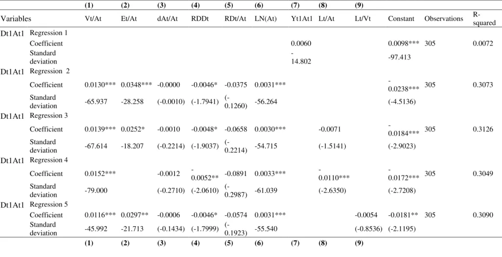
In order to understand how dividends target pay-out changes with variations of profitability, investments and leverage, Table VII - (Appendix – page 51) shows the cross section regression of Yt1At1on Dt1At1. There is a low value on R-squared of 0.0072 and adding intersection terms increases the R-squared to values between 0.2980 and 0.3126.
3.1.1 The relationship between Dividends and Investment: RDtAt
31 therefore it is not possible to make any inference.
For the second investment proxy, dAtAt (3), the expected sign is also negative, as a result of positive changes in total assets when companies channel their resources to growth and consequently there is less cash available to be distributed. However, once again, nothing can be stated, as this is not statistically significant.
Finally, with regards to the last investment proxy, that of VtAt (1), which is the market value of firm t to total assets, the coefficients are statistically significant and they have a positive relationship to dividend pay-outs. However this contradicts the prediction that investment has negative effects on dividend distribution.
Although RDDt (4) is not a proxy, it is a dummy, which assumes a value of 0 if there were R&D expenses, and 1 if there were none. This is statistically significant, and is consistent with the last conclusion. The main inference in this subsection is that Portuguese companies finance investments with debt, avoiding dividend pay-outs. The evidence found suggests that shareholders were probably so levered that they needed to receive dividends, even when this goes against the companies’ interest.
3.1.2 The relationship between Dividends and Profitability Et/At; Vt/At
Both models rely on the prediction that profitable companies pay out more dividends. According to the Pecking Order model, companies with more profits have more capacity to pay out higher values of dividends and maintain the possibility of recovering a low risk of debt as a means of financing investment opportunities. On the other hand, the Trade-Off model points out that paying out dividends will control the agency costs created by cash flows. Besides these differing motives, both agree that profitability is positively related to dividend pay-outs, and thus one would be expected that the investments proxies are positive.
32
regards the other proxy of profitability Vt/At (1), it is also statistically significant in all the regressions of the Table VII (Appendix – page 51). Both the variables have positive coefficients which is consistent with previous literature. Companies with more profitability have higher dividend pay-outs.
3.1.3 The relationship between Dividends and Volatility: ln(At)
Concerning volatility, we find the same predictions for both models, although, once again, for different reasons. The Trade-Off points are a reason for more volatile companies having lower pay-out values than safe companies, due to the fact that they have higher expected bankruptcy costs and consequently less leverage, and also that they finally pay out less dividends. Regarding the Pecking Order model, the purpose is related with the fear of having difficulty raising low risk debt. This variable ln(At) (6) is statistically significant and consistent (smaller companies have higher volatilities), and thus smaller companies will pay outs less dividends. This conclusion is in accordance with that found by Fama & French (2002).
3.2 Second Testing Hypothesis
33
prospects of an industry or the company, or may prefer to satisfy requirements for internal funding. Despite these worries, managers and stakeholders show preference for stabilizing fluctuations of dividend rates, by using outside debt and new equity. Some companies compare the speed of adjustment to the most competitive firms.
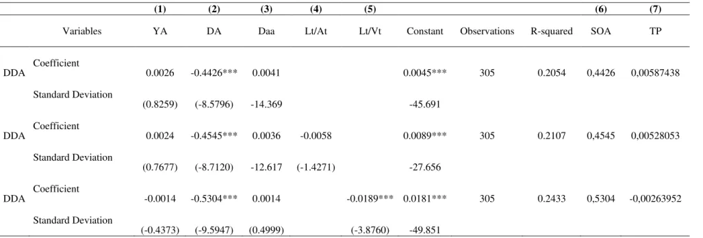
For this hypothesis, i.e., to test whether target dividend pay-outs are adjusted to absorb the short term variation of investments, and also whether firms vary dividend pay-outs from their targets in order to accommodate short term variations in investments, Table VIII (Appendix – page 53) is used, where the independent variable is the DDA, which
equates to the variations of the dividends divided by the assets. The variable TP (7) presented on this table is the Target Pay-Out, which is YA (1) divided by speed of adjustment - SOA (6). When compared to the R-squared for all regressions, this one is situated in an interval of 0.21 to 0.24.
34
simultaneously are all statistically significant. With regards to the main question, it is possible to say that target dividends do not absorb short term variations of investment, as the SOA and DA are not large enough to accomplish a total short term variation.
3.3 Third Testing Hypothesis
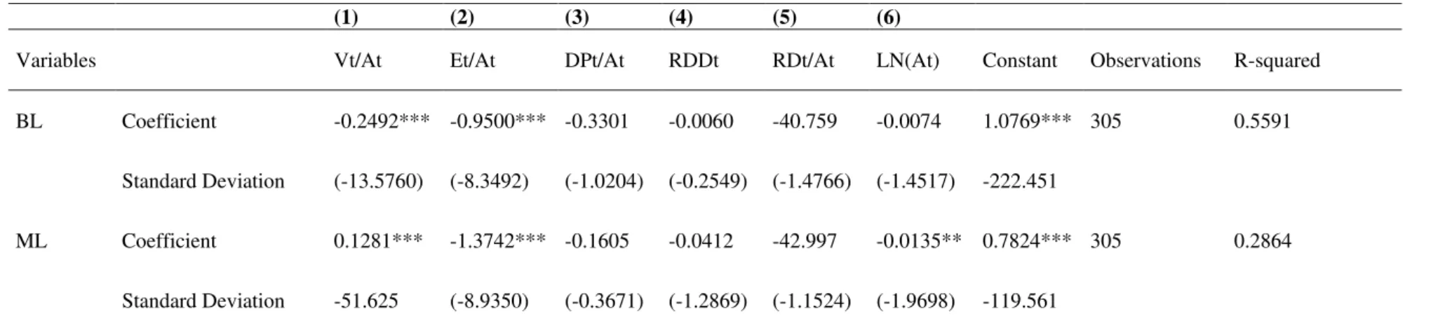
In order to explain the performance leverage, two different measures of leverage are used, the Book and the Market Leverage. For this test hypothesis, it is necessary to resort to Table IX (Appendix –page 54), which include proxies for investment opportunities
leverage VtAt (1), and profitability EtAt (2). The R-squared for Book Leverage regression assumes the value of 0.56, and for Market Leverage, a value of 0.29.
3.3.1 The relationship between Leverage and Profitability VtAt(1) EtAt(2)
In order to relate Leverage with Profitability, we start with VtAt (1), which is a proxy for profitability, and the signs differ for Book and Market Leverage. However, in both cases, they are statistically significant. The coefficient of Book Leverage is negative, and its standard error is -13.6. On the other hand, VtAt (1) is positive when used to explain market leverage, and assumes a standard error of 5.16.
35
If in the short run, dividends and investments are fixed, and if debt financing
is the dominant mode of external financing, then changes in profitability will
be negatively correlated with changes in leverage.
In Harris & Raviv (1991), p. 38. Harris & Raviv (1991) studied this behaviour for several countries. Using these results, and when confronted with their results, we can state that Portuguese companies behave similarly to firms in Japan, Italy, and Canada, and to the opposite of ones in the United Kingdom. These authors found evidence against the static Trade-Off model, which states that more profitable firms should have a higher optimal leverage level. However, extensions of the static Trade-Off theory exist, which state that the negative relationship between profitability and leverage ratios is in fact consistent with the Trade-Off theory. Following Strebulaev’s (2003) train of thought that companies are not constantly adjusting their leverage ratios, on account of transaction costs, companies permit that leverage ratios vary to an interval of values close to the optimal target ratios. For this reason, according to Long Chen & Xinlei Zhao (2005), the market equity values of profitable firms grow faster, leading to the inverse behaviour between profitability and leverage ratios. However, sometimes target companies have to resort to external funds. Thus the negative connection of profitability and leverage ratio might occur on account of firms moving away from their target ratios in the short term.
Another possible explanation of the negative relationship between leverage and profitability is related to the so-called dynamic tax consideration, which proposes that internal funds are less costly than external ones, and for that reason are less attractive, although they permit delaying tax payments. Based on these causes, it is more likely that more profitable firms choose less debt and thus have lower target ratios.
36
companies choose internal funds before raising debt, trying to escape from adverse selection costs.
More profitable firms raise less debt, as they have more internal funds to rely on. The negative inverse connection between profitability and leverage might transmits the idea of a tax benefit, which is also a worry.
3.3.2 The relationship between Leverage and Investment Opportunities RD/At (5),
RDDt(4)
Sometimes, shareholder problems attract situations of inefficient assets substitution- or even under-investment. To oppose this situation, incentives are given to companies that have more investment opportunities, the consequence being that few are under-leveraged. Another reason for the negative relationship between leverage and investment opportunities, according to the Trade-Off model, is the fact that firms can be more flexible towards debt payments as a means of controlling free cashflow problems. Finally, according to Myers (1977), companies with higher levels of leverage are more willing to let profitable investment opportunities pass by, than those with lower levels.
However, as can be observed in Table-3, nothing can be said about the relationship between RD/At (5) for both Book and Market Leverage, as the highest absolute value for standard error presented is only 1.47, and thus they are not statistically significant. Another variable that is not statistically significant and which is not interpretable is RDDt (4)
3.3.3 The relationship between Leverage and Volatility ln(At) (6)
37
and Volatility ln(At) (6), it is possible to make some conclusions, as the coefficient is statistically significant (ML regression). The evidences found is that they have a negative relationship, which is consistent with the complex Pecking Order model. A possible explanation was presented by Fama & French (2002), in that large companies have more ready access to debt market, with lesser costs.
3.3.4 The relationship between Leverage and Non-Debt Tax Shield RDt/At (5) DP/At
(3)
38
4. Conclusions
This study helps to understand how Portuguese companies react with regards to their pay-out policy and leverage when they suffer changes on their capital structure and polices. It must be borne in mind that this is a very controversial subject, which has been studied for decades. To achieve the results, a replication of the methodology made by Fama & French (2002) was applied, in which both Trade-Off and Pecking Order were tested. The regressions used were similar, or identical to those of Fama & French. It is now possible to state that Portuguese companies experience situations in which they behave in accordance with Pecking Order or Trade-Off, and, in some cases, with both of these models. As has been showed before, the literature states that both models share predictions in some occasions, however this happens for different reasons. The predictions of profitability and dividends are in agreement with the two models. The evidence found shows that higher profits result in a higher pay-out of dividends, independent of the underlying theory, whether it be Trade-Off or Pecking Order. This conclusion is also shared by Fama & French (2002)
39
here is that shareholders are probably so leveraged that they are require dividends, even when this goes against the company’s interest.
Another common prediction of those two models regards volatility and dividends, although from different causes. The prediction is that more volatile companies have lower pay-out values than safe companies. This is in accordance with this research, as the size of the company (the proxy for volatility being the smaller the company, the higher the volatility) has a positive and statistically significant coefficient on the regressions. We would also like to emphasize that this conclusion is in agreement with the conclusions of Fama & French (2002).
Regarding the behaviour of target dividend pay-outs, the main question was to know whether they are adjusted to absorb short term variations of investments. With regards to this, we can say that target dividends do not absorb short term variations of investment. Even with values higher than those that were presented by Fama and French 2002 are in evidence, the speed of adjustment is not big enough to bring about a total short term variation.
40
evidence that Portuguese companies with high profitability have lower levels of short and long term book leverage.
With regards to Leverage and Investment Opportunities, we would highlight the need to distinguish between the two variants of the Pecking Order model - the simple and the complex. Concerning the simple PO model and market leverage, there are no predictions; and concerning the simple PO and the BL, a positive relationship is expected. On the other hand, the complex Pecking Order model states a negative relationship. Therefore, the larger the expected investment, the less will be the current Book or Market Leverage. From the Trade-Off theory, the prediction is that the higher the investments opportunity, the less will be the Book or Market Leverage. However, this study does not come to any conclusions about this point, as the coefficient is not statistically significant.
With regards to the relationship between Leverage and Volatility through the Complex Pecking Order model or the Trade Off one, the relationship is negative, i.e., the higher the volatility, the less will be the leverage. Evidence found in this study is in accord with the previous literature, in that companies with more volatility of net cash flow have less book leverage. Regarding Market Leverage, it is not possible to make any inference, as the coefficient is not statistically significant.
There are no statements regarding non-debt tax shield and its relationship with leverage, as the coefficients were not statistically significant.
41
References
• Allen, F., & Michaely, R. (2003). Payout policy. Handbook of the Economics of Finance, 1, 337-429.
• Bradley, M., Jarrell, G. A., & Kim, E. (1984). On the existence of an optimal capital structure: Theory and evidence. The journal of Finance, 39(3), 857-878.´
• Chen, L., & Zhao, X. S. (2005). Profitability, mean reversion of leverage ratios, and capital structure choices. Mean Reversion of Leverage Ratios, and Capital Structure Choices (February 2005).
• DeAngelo, H., & Masulis, R. W. (1980). Optimal capital structure under corporate and personal taxation. Journal of financial economics, 8(1), 3-29.
• DeAngelo, L. E. (1981). Auditor size and audit quality. Journal of accounting and economics, 3(3), 183-199.
• Easterbrook, F. H. (1984). Two agency-cost explanations of dividends. The American Economic Review, 650-659.
• Fama, E. F., & French, K. R. (2001). Disappearing dividends: changing firm characteristics or lower propensity to pay? Journal of Financial economics, 60(1), 3-43.
• Fama, E. F., & French, K. R. (2002). Testing trade‐off and pecking order predictions about dividends and debt. Review of financial studies, 15(1), 1-33.
• Fama, E. F., & MacBeth, J. D. (1973). Risk, return, and equilibrium: Empirical tests. The Journal of Political Economy, 607-636.
• Gordon, M. J. (1959). Dividends, earnings, and stock prices. The Review of Economics and Statistics, 99-105.
42
• Graham, J. R. (1996). Proxies for the corporate marginal tax rate. Journal of Financial Economics, 42(2), 187-221.
• Hakansson, N. H. (1982). To pay or not to pay dividend. Journal of Finance, 415-428. • Harris, M., & Raviv, A. (1991). The theory of capital structure. The Journal of
Finance, 46(1), 297-355.
• Jensen, M. C. (1986). Agency cost of free cash flow, corporate finance, and takeovers. Corporate Finance, and Takeovers. American Economic Review, 76(2). • Jensen, M. C., & Meckling, W. H. (1976). Theory of the firm: Managerial behavior,
agency costs and ownership structure. Journal of financial economics, 3(4), 305-360. • Lintner, J. (1956). Distribution of incomes of corporations among dividends, retained
earnings, and taxes. The American Economic Review, 97-113.
• Miller, M. H. (1977). DEBT AND TAXES*. The Journal of Finance, 32(2), 261-275. • Miller, M. H., & Scholes, M. S. (1978). Dividends and taxes. Journal of financial
economics, 6(4), 333-364.
• Modigliani, F., & Miller, M. H. (1958). The cost of capital, corporation finance and the theory of investment. The American economic review, 261-297.
• Myers, S. C. (1977). Determinants of corporate borrowing. Journal of financial economics, 5(2), 147-175.
• Myers, S. C. (1984). The capital structure puzzle. The journal of finance, 39(3), 574-592.
• Myers, S. C., & Majluf, N. S. (1984). Corporate financing and investment decisions when firms have information that investors do not have. Journal of financial economics, 13(2), 187-221.
43
• Strebulaev, I. A. (2003). Many faces of liquidity and asset pricing: Evidence from the US Treasury securities market.
44
Appendix
Table I - Population of the study - list of Companies.
VAA Vista Alegre Atlantis SGPS (VAFK PL)
VAA Vista Alegre Atlantis SGPS (VAF PL) - By Segment SAG GEST-Solucoes Automovel Globais SGPS SA (SVA PL) Sonae Industria SGPS SA (PL)
Sonae Capital SGPS SA (SONC PL) Sonae SGPS SA (SON PL)
Sonaecom - SGPS SA (SNC PL)
Semapa-Sociedade de Investimento e Gestao (SEM PL) SDC - Investimentos SGPS SA (SDCAE PL)
SDC - Investimentos SGPS SA (SDCP PL) Toyota Caetano Portugal SA (SCT PL)
REN - Redes Energeticas Nacionais SGPS SA (RENE PL) Reditus-SGPS SA (RED PL)
Portugal Telecom SGPS SA (PTC PL) Portucel SA (PTI PL)
Sociedade Comercial Orey Antunes SA (ORE PL) NOS SGPS (NOS PL)
Novabase SGPS SA (NBA PL) Mota-Engil SGPS SA (EGL PL) Grupo Media Capital SGPS (MCP PL) Martifer SGPS SA (MAR PL)
Lisgrafica Impresso & Artes (LIG PL) Jeronimo Martins SGPS SA (JMT PL) Impresa SGPS SA (IPR PL
INAPA - Investimentos Participacoes e Gestao SA (INA PL) Impresa SGPS SA (IPR PL)
Ibersol SGPS SA (IBS PL)
Imobiliaria Construtora Grao-Para SA (GPA PL)
Global Intelligent Technologies SGPS S.A. (GLINT PL) Galp Energia SGPS SA (GALP PL)
Futebol Clube Do Porto (FCP PL)
F. Ramada Investimentos SGPS SA (RAM PL) Estoril Sol SGPS SA (ESON PL)
Estoril Sol SGPS SA (ESO PL) EDP Renovaveis SA (EDPR PL)
EDP - Energias de Portugal SA (EDP PL) Corticeira Amorim SGPS SA (COR PL)
Compta-Equipamento e Servicos de Informatica SA (COMAE PL) Cofina SGPS SA (CFN PL)
45
Table II - Pecking Order vs Trade-Off Predictions
Source: Author´s construction, based on the previous literature
Predictions Pecking Order Trade-Off
Financing
Companies will always choose the least expensive method of financing the company. Companies choose how to finance themselves through:
1. retained earnings
2. safe debt
3. risky debt
4. equity
Dividend and leverage decisions are based on a Trade-Off between a number of costs and benefits. The predictions are organized by four stages:
• bankruptcy costs
• taxes
• free cash flow agency
problems
• stockholder/bondhol
der agency problems
Dividend Pay-outs and
Investment
Firms with higher ratios of investment to earning have less dividend distribution.
Firms with more investments have lower dividend pay-outs.
Dividend Pay-outs and
Profitability
With higher profitability ratios, companies have more dividend pay-outs.
With higher profitability ratios, companies have more dividend pay-outs.
Dividend Pay-outs and
Volatility.
Larger companies have less volatility and higher pay-outs
Volatile companies have lower pay-out values than safe companies.
Dividends and
Leverage Higher leverage, less dividend pay-outs.
The higher the leverage (Book or Market), the less the dividend payouts.*
Volatility and Leverage
Complex Pecking Order- Companies with more-volatile earnings have less current debt (Book or Market Leverage).
Companies with more-volatile earnings should carry less debt.
Profitability and Leverage
More-profitable companies will have lower leverage.
Book Leverage: A Positive
Relation between Book Leverage and Profitability.
Market Leverage: No
prediction, between Market Leverage and Profitability because Market Value increases with profitability.
Financing Non-debt tax
shield and Leverage
46
Predictions Pecking Order Trade-Off
Leverage and Investments
Simple Pecking Order:
Book Leverage: Higher investment,
higher Book Leverage
Market Leverage:No prediction
Complex Pecking Order
Book Leverage:Larger expected
investment, less current leverage.
Market Leverage:Larger expected
investment, less current leverage.
Book Leverage:
Negative relation between Book Leverage and Investment Opportunity.*
Market Leverage:
Negative relation between Leverage and Investment Opportunity.*
Target leverage
Does not have obvious leverage targets. However dividends are inelastic, and thus short-term variations in earnings or investments are presumed to be by incorporation of variations of leverage.
Companies have leverage targets and that the level of leverage is mean, reverting around this target.
47
Table III - Variables Description
Source: Author’s constructions, based on Fama and French (2002)
Variable's Name Variable Formula
Total asset at t moment At Short term Asset t + Long term Assets t Changes on Total Asset at moment t DAt Asset t – Asset t-1
Dividends at t moment D Value of dividend Earnings before interest at moment t Et EBIT-Tax expenses Changes of EBI at moment t DEt EBIt-EBIt-1
Earnings before interest and taxes at moment t ETt EBITDA - Depreciations and Amortizations Changes of EBIT at moment t DETt EBITt-EBITt-1
Market Equity at moment t Met Number of shares t * Stock Price t
Market value of Firm at moment t Vt Liabilities – deferred taxes and investments tax credit + preferred stocks + market equity R & D Expenditures at moment t RDt Value of R & D Expenditures
Dummy of R & D Expenditures at moment t RDDt Takes the value 0 if there is R & D Expenditures and the value 1 otherwise Depreciation Expense at moment t DPt Value of Depreciations
Liabilities at moment t Lt Short term debt t+ long term debt t Number of shares outstanding at moment t NSt Number of Shares
Stock price at moment t SPt Value of stock Price
LN(asset) at moment t Ln(At) Logarithm of the Asset´s Value Book Equity at moment t BE Value of Book Equity
Variations of Stock Price at moment t DSPt Stock Price t - Stock Price t-1
48
Table IV - Proxies
Source: Author’s constructions, based on Fama and French (2002)
Proxies Variable's Name Variable Formula
Profitability
Earnings before interest and taxes t / total assets t. ETtAt ETt/At Earnings before interest t / total assets t. EtAt Et/At Market value of firm t / total assets t. VtAt Vt/At
Non-debt tax Shield R & D expenditures t / value of assets t. RdtAt RDt/At Depreciations expenses t / total assets t. DPtAt DPt/At
Investment opportunities
49
Table V - Ratios
Source: Author’s constructions, based on Fama and French (2002)
Variable's Name Variable Formula
Market Leverage at moment t. LtVt Lt/Vt
Book Leverage at moment t LtAt Lt/At
Dividends t+1/ total Assets t+1 Dt1At1 Dt1/At1 Variation of Market Capitalization t+1/ total Assets t+1 Yt1At1 Yt1/At1 (Dividends t+1 – Dividends t)/ total Assets t+1 DDA (Dt1 - Dt)/At1 Dividends t/ total Assets t+1 Dt/At1 DA Dt/At1 (Total Asset t+1 – total Assets t)/ total Assets t+1 (At1 - At)/At1 Daa (At1 - At)/At1 Variation of Market Capitalization t+1/ total Assets t YA Yt1/ At
Target Book leverage moment t+1 BL Liabilities t+1/ total Assets t+1 Target Market leverage moment t+1 ML Liabilities t+1/ Market value of
Firm t
Variation of Liabilities to assets ratio between t+1 and t LAL Lt1/At1 - LtAt
Changes of EBI moment t+1 Det Et+1 – Et
Changes of EBI moment t+1 divided by total assets on moment t +1 DEA (Et+1 – Et )/At+1 Changes of Total between t and t-1t to Total assets t+1 DAA dAt/At1
50
Table VI - Descriptive statistics
Source: Author’s constructions, based on the Bloomberg database.
51
Table VII - Fama and French (2002) Regressions used to understand how Target Pay-Outs behave when they are a function
of investment opportunities, profitability and volatility proxies.
Statistics in parentheses; *** p<0.01, ** p<0.05, * p<0.1;
Source: Author’s constructions based on Bloomberg database and Fama and French (2002).
(1) (2) (3) (4) (5) (6) (7) (8) (9)
Variables Vt/At Et/At dAt/At RDDt RDt/At LN(At) Yt1At1 Lt/At Lt/Vt Constant Observations R-squared
Dt1At1 Regression 1
Coefficient 0.0060 0.0098*** 305 0.0072
Standard deviation
-14.802 -97.413
Dt1At1 Regression 2
Coefficient 0.0130*** 0.0348*** -0.0000 -0.0046* -0.0375 0.0031***
-0.0238*** 305 0.3073 Standard
deviation -65.937 -28.258 (-0.0010) (-1.7941)
(-0.1260) -56.264 (-4.5136)
Dt1At1 Regression 3
Coefficient 0.0139*** 0.0252* -0.0010 -0.0048* -0.0658 0.0030*** -0.0071
-0.0184*** 305 0.3126 Standard
deviation -67.614 -18.207 (-0.2214) (-1.9037)
(-0.2214) -54.715 (-1.5141) (-2.9023)
Dt1At1 Regression 4
Coefficient 0.0152*** -0.0012
-0.0052** -0.0891 0.0033***
-0.0110***
-0.0172*** 305 0.3049 Standard
deviation -79.000 (-0.2710) (-2.0610)
(-0.2987) -61.039 (-2.6350) (-2.7208)
Dt1At1 Regression 5
Coefficient 0.0116*** 0.0297** -0.0006 -0.0046* -0.0574 0.0031*** -0.0054 -0.0181** 305 0.3090 Standard
deviation -45.992 -21.713 (-0.1434) (-1.7999)
(-0.1923) -55.540 (-0.8536) (-2.1195)
52
Variables Vt/At Et/At dAt/At RDDt RDt/At LN(At) Yt1At1 Lt/At Lt/Vt Constant Observations R-squared
Dt1At1 Regression 6
Coefficient 0.0111*** -0.0010 -0.0049* -0.0887 0.0034***
-0.0114** -0.0139* 305 0.2980 Standard
deviation -43.945 (-0.2143) (-1.9156)
(-0.2957) -63.394 (-1.9857) (-1.6640)
53
Table VIII - Lintner model regression to explain variations in Dividend Targets
Statistics in parentheses; *** p<0.01, ** p<0.05, * p<0.1;
Source: Author’s constructions based on Fama and French (2002)
(1) (2) (3) (4) (5) (6) (7)
Variables YA DA Daa Lt/At Lt/Vt Constant Observations R-squared SOA TP
DDA Coefficient 0.0026 -0.4426*** 0.0041 0.0045*** 305 0.2054 0,4426 0,00587438 Standard Deviation
(0.8259) (-8.5796) -14.369 -45.691
DDA Coefficient 0.0024 -0.4545*** 0.0036 -0.0058 0.0089*** 305 0.2107 0,4545 0,00528053 Standard Deviation
(0.7677) (-8.7120) -12.617 (-1.4271) -27.656
DDA Coefficient -0.0014 -0.5304*** 0.0014 -0.0189*** 0.0181*** 305 0.2433 0,5304 -0,00263952
54
Table IX - Fama and French Regression to understand the behaviour of Book and Market Leverage when they are a function
of investment opportunities, profitability and volatility proxies
Statistics in parentheses; *** p<0.01, ** p<0.05, * p<0.1;
Source: Author’s constructions based on Bloomberg database and Fama and French (2002)
(1) (2) (3) (4) (5) (6)
Variables Vt/At Et/At DPt/At RDDt RDt/At LN(At) Constant Observations R-squared
BL Coefficient -0.2492*** -0.9500*** -0.3301 -0.0060 -40.759 -0.0074 1.0769*** 305 0.5591
Standard Deviation (-13.5760) (-8.3492) (-1.0204) (-0.2549) (-1.4766) (-1.4517) -222.451
ML Coefficient 0.1281*** -1.3742*** -0.1605 -0.0412 -42.997 -0.0135** 0.7824*** 305 0.2864
Standard Deviation -51.625 (-8.9350) (-0.3671) (-1.2869) (-1.1524) (-1.9698) -119.561