Essays on international trade

(1)

FUNDAC

¸ ˜

AO GETULIO VARGAS

ESCOLA de P ´

OS-GRADUAC

¸ ˜

AO em ECONOMIA

Rafael Amaral Ornelas

Essays on International Trade

Rio de Janeiro 2019

(2)

Rafael Amaral Ornelas

Essays on International Trade

Tese para obten¸cão do grau de doutor apresentada à Escola de Pós-Graua¸cão em Economia

´

Area de concentra¸c˜ao: Com´ercio Interna-cional

Orientador: Afonso Arinos de Mello Franco Neto

Rio de Janeiro 2019

(3)

Dados Internacionais de Catalogação na Publicação (CIP) Ficha catalográfica elaborada pelo Sistema de Bibliotecas/FGV

Ornelas, Rafael Amaral

Essays on international trade / Rafael Amaral Ornelas. – 2019. 149 f.

Tese (doutorado) - Fundação Getulio Vargas, Escola de Pós-Graduação em Economia.

Orientador: Afonso Arinos de Mello Franco Neto. Inclui bibliografia.

1. Comércio internacional. 2. Vantagem comparativa (Comércio

Internacional). I. Franco Neto, Afonso Arinos de Mello.II. Fundação Getulio Vargas. Escola de Pós-Graduação em Economia. III. Título.

CDD – 382.08

(4)

(5)

Resumo

Esta tese é composta de três artigos, cada um correspondendo a um cap´ıtulo. No primeiro cap´ıtulo, eu desenvolvo um modelo de equil´ıbrio geral de comércio internacional com vantagem comparativa, em que as firmas têm produtividades heterogêneas, mark-ups variáveis e existem duas indústrias diferentes. Eu uso esse modelo para obter diferentes implica¸cões de bem-estar, considerando mark-ups variáveis e utilizando preferências translog em vez das preferências CES. Eu também apresento um exerc´ıcio numérico para avaliar as variáveis endógenas do modelo quando os custos de comércio são reduzidos. No segundo cap´ıtulo, uso modelos teóricos de comércio a lá Melitz /Chaney para avaliar o impacto de Barreiras Não-Tarifárias (NTB) no comércio e no bem-estar da economia, para isso, calculo o trade-off entre custos variáveis e fixos quando um pa´ıs ou um bloco comercial impõe uma regula¸cão NTB. No terceiro cap´ıtulo, utilizo dados agregados de comércio para avaliar o impacto de uma regula¸cão NTB que foi imposta pela União Européia para regulamentar produtos espec´ıficos de carne. Também testo um resultado anal´ıtico do modelo desenvolvido no cap´ıtulo anterior.

Palavras-chave: Comércio Internacional. Vantagem Comparativa. Firmas Heterogêneas. Mark-ups variáveis. Barreiras Não-Tarifárias. Modelo Gravitacional. Produtos Agr´ıcolas.

(6)

Abstract

This thesis is composed of three articles, each one corresponding to a chapter. In the first chapter I develop a general equilibrium model of international trade with comparative advantage, where firms have heterogeneous productivities, variable mark-ups and there are two different industries. I use this model to obtain different welfare implications considering variable markups and using translog preferences instead of CES preferences. I also present a numerical exercise to asses endogenous variables of the model when trade costs fall. In the second chapter I use theoretical Melitz/Chaney-like trade models to evaluate the impact of Non-Tariff Barrier (NTB) in trade and welfare at the economy by calculating the trade off between variable and fixed costs when a country or a trade bloc imposes a NTB regulation. In the third chapter I use aggregate trade data to asses the impact of a NTB regulation imposed by the European Union to regulate specific beef products. I also test an analytical outcome of the model developed in the previous chapter. Keywords: International Trade. Comparative Advantage. Heterogeneous Firms. Variable Mark-ups. Non-Tariffs Barrier Regulation. Gravity Model. Agricultural Products.

(7)

List of Figures

1.1 Zero-profit and export cut-offs . . . 29

1.2 Average productivity . . . 30

1.3 Average firm output . . . 30

1.4 Differences in comparative advantage . . . 31

1.5 Exporting probability . . . 31

1.6 Mass of firms (domestic varieties) . . . 32

1.7 Mass of entrants . . . 32

1.8 Welfare evaluation . . . 33

(8)

List of Tables

3.1 Regulated vs non-regulated meat products . . . 141

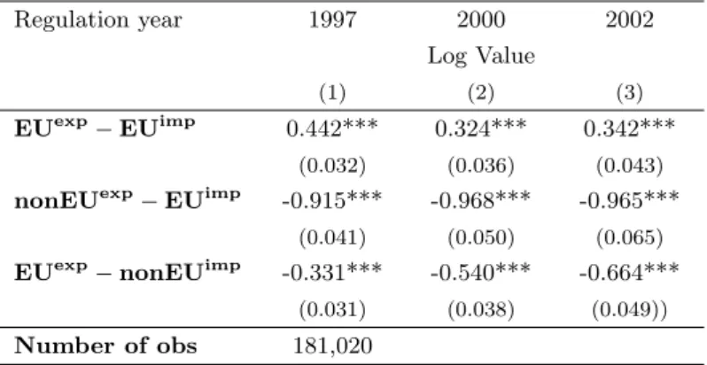
3.2 NTB regulation impacts on exports and imports . . . 142

3.3 NTB regulation impacts on specific trade flows . . . 142

3.4 Robustness: NTB regulation impacts on exports and imports . . . 143

(9)

Comparative Advantage,

Heterogeneous Firms and Variable

Mark-ups

1.1 Introduction

Firms apply different mark-ups on their products. Many factors influence firms’ decision re-garding the size of the mark-up that the firm can charge for each product: productivity, input costs, size of the firm, competition, industry characteristics, comparative advantages, and other factors. What are the trade outcomes in an environment where all those factors are considered? After Melitz(2003), many authors have used his model of heterogeneous firms as a starting point for their own models of international trade. 1 By using Melitz’s model, researchers can obtain results for trade gains through two channels. On the one hand, as in Melitz (2003), trade induces competition for scarce production factors, (e.g., labor). Thus, real wages are bid up by the relatively more productive firms, which expand production to serve foreign markets.

Bernard et al.(2007) obtain trade gains through this channel, but their model also focuses on comparative advantage, which magnifies trade gains in the comparative advantage industry. On the other hand, inMelitz and Ottaviano (2008), and in Rodr´ıguez-L´opez (2011), foreign firms increase competition in the domestic market, which shifts up residual demand price elasticities for all firms at any given demand level. However, competition for production factors plays no

1

Other international trade models also incorporate heterogeneous firms: seeBernard et al. (2003); Helpman

(12)

2

role in those models.

The differences in the origin of trade gains between those models is found in the utility of consumers. The first group of models, which follows Melitz (2003), uses CES utility and does not allow price elasticity to vary. When it does vary, we have endogenous mark-ups, and trade gains via the second channel (the path taken by the second group). In this paper, we build a model that fits both channels for trade gains, and also imposes factor intensity differences across industries. Thus, comparative advantage differences have a role in the economy. The main contribution of this paper is to combine the two channels (competition for production factors and competition shifts up price elasticities) into a unique framework. We analyze international trade in an environment that allows endogenous mark-ups and yet have two industries and comparative advantage effects.

We develop a monopolistic competitive model of trade with heterogeneous firms, two in-dustries, and endogenous mark-ups. This environment allows our model to obtain trade gains through both channels. Firm heterogeneity is introduced similarly toMelitz(2003), through pro-ductivity differences. We introduce endogenous mark-ups using translog expenditure functions on the demand side. This technique was introduced inFeenstra (2003), and is used inArkolakis et al.(2010) and inRodr´ıguez-L´opez (2011). Translog expenditure functions are useful because they allow price elasticity to vary; this differentiates it from CES, although preference is still homothetic. We particularly follow three papers: Bernard et al. (2007), Melitz and Ottaviano

(2008), andRodr´ıguez-L´opez(2011).

As in Melitz and Ottaviano (2008), in our model, market size and the openness of the economy affect the toughness of competition in a market, which then feeds back into the selection of heterogeneous producers and exporters in that market2_{. The fact that we have two industries}

also influences this selection. We are able to find similar trade outcomes to those found in

Bernard et al.(2007) with the advantage that in our model the mark-ups are free to vary. First, we develop a closed-economy version of our model. As inMelitz and Ottaviano(2008), but differently from Melitz (2003), market size induces important changes in the equilibrium distribution of firms and their performance measures. Larger markets require higher productivity cutoffs, and larger markets have larger firms with higher profits. We then present an open economy with costly trade.

When the economy moves from autarky to costly trade, we show that larger markets still

ex-2

Asplund and Nocke(2006) investigate the effect of market size on the entry and exit rates of heterogeneous firms.

(13)

3

hibit larger and more productive firms, lower prices, and lower mark-ups. We also find the same results as those inBernard et al.(2007). When countries move simultaneously from autarky to costly trade, firms’ export opportunities increase, which promotes greater entry from the com-petitive fringe. However, the mass of domestic producers decreases in both countries. As result, most productive firms start to sell in the foreign market. The proportion of firms exporting will be higher in the comparative advantage industry. The productivity cut-off necessary to produce increases, and the most productive firms start to export, causing the aggregate productivity level in each industry to increase.3 This result is higher in the comparative-advantage industry and intensifies its ex ante comparative advantage, which raises trade gains. After opening the market, all firms set smaller mark-ups, an effect that is higher in firms from the comparative ad-vantage industry. However, average mark-ups in both industries do not change. These findings contrast with the homogeneous-firm imperfect competition model of Helpman and Krugman

(1987)4, where industry productivity remains constant and, depending on the value of fixed and variable trade costs, either all or no firms export when there is trade liberalization.

Considering distributional implications, our framework reproduces the Stoper-Samuelson theorem, but also finds another effect. As a consequence of aggregate productivity growth, average price of the variety is reduced in each industry and thereby elevates real income for both factors. Thus, even if the real wage of the scarce factor falls as a result of trade opening, its decline is lower than it would be in a Neoclassical model. The falling of all mark-ups of the remaining firms reduces the price for each variety, but once the average mark-up is held constant there is no effect on prices index.

As in Bernard et al. (2007), our approach also generates predictions about the impact of trade liberalization on job turnover that are different from those obtained in a Neoclassical model. We show that a reduction in trade barriers encourages simultaneous job creation and job destruction in all industries, but gross and net job creation vary with country and industry characteristics.

In order to illustrate the main trade outcomes of the model, we construct a numerical exercise. We calibrate our model to a symmetric environment and let trade costs vary. In this numerical exercise, we calculate a weighted average mark-up. Differently from the average mark-up, it

3

Empirical studies strongly confirm these selection effects of trade (only the most productive firms export).

For example, seeClerides et al.(1998);Bernard and Bradford Jensen(1999);Aw et al.(2000);Pavcnik (2002);

andBernard et al.(2006).

4

Other works on imperfect competition and comparative advantage includeKrugman(1981);Helpman(1984);

(14)

4

does vary when trade costs change, providing a useful intuition for the impact of endogenous mark-up in the present environment. We found that when competition gets “tougher”, weighted average mark-up falls, the same as the average mark-up in Melitz and Ottaviano(2008).

When mark-ups are endogenous, more productive firms set higher mark-ups. Bernard et al.

(2003) also incorporate firm heterogeneity and endogenous mark-ups in their model. However, the distribution of mark-ups is invariant to country characteristics and to geographic barriers.

Melitz and Ottaviano(2008) develop a non-degenerate distribution of mark-ups, which depends on country characteristics and on geographic barriers, but they have only one industry and there are no effects related to comparative advantage and they analyze asymmetric trade liberalization scenarios. Rodr´ıguez-L´opez (2011) presents a sticky-wage model of exchange rate pass-through with heterogeneous producers and endogenous mark-ups. Arkolakis et al.(2010) provide a simple example of an economy where consumers have the Translog Expenditure Function utility, and firm-level productivity distribution is the Pareto distribution. Thus, their environment is similar to ours. However, they also have only one industry in their model. In this paper we focus on the effects that variable mark-ups cause in an economy when it moves from closed to open economy. Our model has two industries, and we also analyze the effect of endogenous mark-ups in this environment with comparative advantage effects. Our approach permits us to find closed-solutions for all endogenous variables of the equilibrium.

? propose a model of monopolistic competition with additive preferences and variable marginal costs. They use the concept of “relative love for variety” (RLV) to provide a full characterization of the free-entry equilibrium. In their work they show that when we use CES utility, as the elasticity of substitution is constant, RLV will also be constant. This is a specific case where prices and mark-ups are not affected by firm entry and market size. However, they are interested in those cases where RLV is free to vary. Our model goes in this direction and our results are in line with the results in ? when RLV increases.

InArkolakis et al. (2012), the authors analyze if micro-level data have had a profound influ-ence on research in international trade over the last years. They find that, although models have become more detailed, the amount of welfare gains does not change much when compared with those obtained by simpler models, such as the Armington model. They make some assumptions (e.g., CES utility) that we do not use in our model, but Arkolakis et al. (2010) shows that the main result holds in a model similar to that used inRodr´ıguez-L´opez(2011).

(15)

5

models that allow variable mark-ups, including models with the continuous translog expenditure function. They find that gains from trade liberalization are weakly lower than those predicted by the models with constant markups considered inArkolakis et al.(2012). They argue that “there is incomplete pass-through of changes in marginal costs from firm to consumers”. Edmond et al.

(2018) take a similar track, finding welfare costs of mark-ups in an environment where these mark-ups are variable. In their model, mark-ups reduce welfare mainly because the aggregate mark-up distortion acts like an uniform output tax. They also do not account for comparative advantage effects. On the other hand Edmond et al. (2015) find that trade can significantly reduce mark-up distortions because greater competition may reduce misallocation and increase aggregate productivity. However, they consider a situation of oligopolistic competition. They highlight that, given the misallocation of resources, their model predicts larger procompetitive gains if, within a given sector, domestic and foreign producers have relatively similar levels of productivity. This is not true in our environment, in which comparative advantage plays an important role.

Mayer et al. (2014) build a model of multi-product firms that highlights how market size and geography affect both a firm’s exported product range and its exported product mix across destinations. They find that tougher competition shifts the entire distribution of mark-ups down across products and skews export sales toward better-performing products. This is similar to our results, in which tougher competition induces firms to set lower mark-ups and the “better-performing” firms export more.

Finally, our model could be a more useful benchmark than the existing theory for predicting the pattern of trade. The Neoclassical standard Heckscher-Ohlin-Vanek model presents poor empirical performance, because it does not capture the existence of trading costs, factor price inequality, and the variation in technology and productivity across countries5.

The remainder of the paper is structured as follows. Section 2 introduces the model for a closed economy. Section 3 expands the model to a costly trade economy. In section 4, we present the results that we find when the economy moves from autarky to costly trade. Section 5 presents our numerical exercise, and section 6 concludes the study.

5

See, among others, Bowen et al.(1987); Trefler(1993); Trefler(1995); Davis and Weinstein(2001); Schott

(16)

6

1.2 Closed Economy

In this section we present a closed-economy model, so there are no exporters in this section. Consider an economy with 𝐿 consumers.

1.2.1 Consumption

The representative consumer’s utility in the upper tier is given by a Cobb-Douglas utility func-tion. In the lower tier, the utility is given by the continuous translog expenditure function as in Rodriguez-Lopez (2011). Preferences are defined for a continuum of differentiated goods. In each industry, ℎ = {𝑥,𝑦}, there is a set of goods, Ωℎ. Each set includes the total number of

actual, and potential (not yet invented) goods, and has a measure of ˜𝑁ℎ. Let Ω

′

ℎ, with measure

𝑁ℎ, be the subset of Ωℎ that contains the set of goods that are available for purchase in the

economy. Utility level is 𝑈 , and 𝑃ℎ is the price index of industry ℎ. Then the expenditure

function of the representative consumer is given by:

ln 𝐸 = 𝑙𝑛𝑈 + 𝛼𝑥ln 𝑃𝑥+ 𝛼𝑦ln 𝑃𝑦. Where 𝛼𝑥+ 𝛼𝑦 = 1, and; ln 𝑃ℎ= 1 2𝛾ℎ𝑁ℎ + 1 𝑁ℎ ∫︁ 𝑖∈Ω′_ℎ ln 𝑝𝑖ℎ𝑑𝑖 + 𝛾ℎ 2𝑁ℎ ∫︁ 𝑖∈Ω′_ℎ ∫︁ 𝑗∈Ω′_ℎ ln 𝑝𝑖(ln 𝑝𝑗− ln 𝑝𝑖)𝑑𝑗𝑑𝑖. (1.1)

Where 𝛾ℎ > 0 indicates the degree of substitutability between goods: larger values of 𝛾ℎ

imply higher substitutability between goods in that industry (low differentiation). Consumers exhibit “love of variety”: when the set of goods in the economy, 𝑁ℎ, is larger, the necessary

expenditure to achieve utility U is lower.

In this economy we have two kind of agents, skilled workers and unskilled workers. Each kind of worker will offer one unit of labor. The size of the economy is given by 𝐿 = 𝐿𝑠+ 𝐿𝑢. 𝑤𝑘

is the wage earned by the worker, 𝑘 = {𝑠,𝑢}. The aggregate income in the economy is given by 𝐼 = 𝑤𝑠𝐿𝑠 + 𝑤𝑢𝐿𝑢.

Using Shephard’s lemma, the share 𝑠𝑖ℎ of good 𝑖 from industry ℎ in the expenditure of the

(17)

7 𝑠𝑖ℎ= 𝜕 ln 𝐸 𝜕 ln 𝑝𝑖ℎ = 𝛼ℎ (︃ 1 𝑁ℎ + 𝛾ℎ 𝑁ℎ ∫︁ 𝑗∈Ω′_ℎ 𝑙𝑛𝑝𝑗ℎ𝑑𝑗 − 𝛾ℎln 𝑝𝑖ℎ )︃ .

Note that when 𝑠𝑖ℎ= 0 we have that 𝑝𝑖ℎ= ^𝑝ℎ, where ^𝑝ℎ= 𝑒𝑥𝑝

(︁

1

𝛾ℎ𝑁ℎ + ̃︂𝑙𝑛𝑝ℎ

)︁

is the chock-off price. This is the highest price that a firm 𝑖 can charge in industry ℎ, and sell anything.

̃︂ 𝑙𝑛𝑝ℎ= _𝑁1_ℎ

∫︀

𝑗∈Ω′_ℎ𝑙𝑛𝑝𝑗ℎ𝑑𝑗 is the average log price. Then,

𝑠𝑖ℎ= 𝛼ℎ𝛾ℎ𝑙𝑛

(︂ ^𝑝ℎ

𝑝𝑖ℎ

)︂

. (1.2)

Using1.2, we can write the demand for a good 𝑖 in industry ℎ.

𝑞𝑖ℎ= 𝛾ℎln (︂ ^𝑝ℎ 𝑝𝑖ℎ )︂ 𝛼ℎ𝐼 𝑝𝑖ℎ .

From now on, 𝐼ℎ= 𝛼ℎ𝐼, and 𝛼𝑥= 𝛼 and 𝛼𝑦 = 1 − 𝛼.

1.2.2 Profit Maximizing Price

Each firm 𝑖 has a constant marginal cost 𝑐𝑖ℎ. Thus, firms solve the following maximization

problem:

𝑚𝑎𝑥𝑝𝑖ℎ𝑝𝑖ℎ𝑞𝑖ℎ− 𝑐𝑖ℎ𝑞𝑖ℎ.

The solution is 𝑝𝑖ℎ= [1 + 𝑙𝑛(^𝑝ℎ/𝑝𝑖ℎ)]𝑐𝑖ℎ. Note that,

𝑝𝑖ℎ 𝑐𝑖ℎ = 1 + ln (︂ ̂︀ 𝑝ℎ 𝑐𝑖ℎ 𝑐𝑖ℎ 𝑝𝑖ℎ )︂ , 𝑝𝑖ℎ 𝑐𝑖ℎ 𝑒 𝑝𝑖ℎ 𝑐𝑖ℎ ₌ 𝑝̂︀ℎ 𝑐𝑖ℎ 𝑒, 𝑝𝑖ℎ 𝑐𝑖ℎ = 𝒲 (︂ ̂︀ 𝑝ℎ 𝑐𝑖ℎ 𝑒 )︂ .

Where 𝒲(𝑧) is the Lambert function defined as the inverse of 𝑥 = 𝑧𝑒𝑧 for 𝑥 > 06. Thus;

𝑝𝑖ℎ= 𝒲 (︂ ^𝑝ℎ 𝑐𝑖ℎ 𝑒 )︂ 𝑐𝑖ℎ. (1.3)

Using1.3we define the mark-up of firm 𝑖 in industry ℎ as

6_{the Lambert function has the properties of 𝒲}

(18)

8 𝜇𝑖ℎ≡ 𝒲 (︂ ^𝑝ℎ 𝑐𝑖ℎ 𝑒 )︂ − 1. (1.4) Then, 𝑝𝑖ℎ= (1 + 𝜇𝑖ℎ)𝑐𝑖ℎ, (1.5) 𝑙𝑛𝑝𝑖ℎ= 𝑙𝑛^𝑝ℎ− 𝜇𝑖ℎ, (1.6) 𝑠𝑖ℎ= 𝛾ℎ𝜇𝑖ℎ. (1.7) 1.2.3 Production

Each industry ℎ = {𝑥,𝑦} uses skilled and unskilled labor with different intensities. There are factor intensity differences across industries. Industry 𝑥 is intensive in skilled labor and industry 𝑦 in unskilled labor, thus 𝛽𝑥> 𝛽𝑦.

The marginal cost of production of each firm in each industry is given by:

𝑐ℎ(𝜙) =

(𝑤𝑠)𝛽ℎ(𝑤𝑢)1−𝛽ℎ

𝜙 .

In this economy, production will follow Melitz (2003) and Bernard, Redding and Schott (2007). Each firm will invest a sunk cost 𝑓𝐸(𝑤𝑠)𝛽ℎ(𝑤𝑢)1−𝛽ℎ, to draw a productivity 𝜙 from a

distribution 𝑔(𝜙) to 𝜙 ∈ [𝜙, + ∞) seeking to produce in industry ℎ. Note that production and investments in the industry both use production factors at the same proportion in each industry, given wages. Price in the domestic market is given by:

𝑝ℎ(𝜙) = (1 + 𝜇ℎ(𝜙))

(𝑤𝑠)𝛽ℎ(𝑤𝑢)1−𝛽ℎ

𝜙 . (1.8)

The mark-up is:

𝜇ℎ(𝜙) = 𝒲 ⎛ ⎝ ^ 𝑝ℎ (𝑤𝑠)𝛽ℎ(𝑤𝑢)1−𝛽ℎ 𝜙 𝑒 ⎞ ⎠− 1. (1.9)

Output, 𝑦ℎ(𝜙), revenue, 𝑟ℎ(𝜙), and profit, 𝜋ℎ(𝜙), of each firm can be calculated substituting

(19)

9 𝑦ℎ(𝜙) = 𝛾ℎ𝐼ℎ 𝑐ℎ(𝜙) (︂ 𝜇ℎ(𝜙) 1 + 𝜇ℎ(𝜙) )︂ , 𝑟ℎ(𝜙) = 𝑝ℎ(𝜙)𝑦ℎ(𝜙) = 𝛾ℎ𝐼ℎ𝜇ℎ(𝜙), 𝜋ℎ(𝜙) = 𝛾ℎ𝐼ℎ 𝜇ℎ(𝜙)2 1 + 𝜇ℎ(𝜙) .

More productive firms set lower prices, earn higher revenues, make higher profits, and set higher mark-ups.

1.2.4 Cutoff Productivity Levels

For each industry, the cutoff 𝜙ℎ determines which firms have a productivity high enough to

produce. Firms only produce if their profit is non-negative, that is, if 𝜙 ≥ 𝜙ℎ, where 𝜙ℎ =

inf{𝜙 : 𝜇ℎ(𝜙) > 0}. Thus; 𝜙ℎ = (𝑤𝑠)𝛽ℎ(𝑤𝑢)1−𝛽ℎ ^ 𝑝ℎ .

The productivity cutoff is higher the lower the chock-off price, and the higher the input costs. To proceed further we adopt the Pareto distribution for productivities, as in Melitz and Ottaviano(2008). The density function for 𝜙 ∈ [𝜙, ∞], where 𝑘 ≥ 1, is:

𝑔(𝜙) = 𝑘𝜙

𝑘

𝜙𝑘+1,

and the distribution function is,

𝐺(𝜙) = 1 − (︂_𝜙

𝜙 )︂𝑘

.

Thus, the distribution of those firms that draw a productivity 𝜙 high enough to produce in industry ℎ is 𝑔(𝜙|𝜙 > 𝜙ℎ) = ⎧ ⎪ ⎨ ⎪ ⎩ 𝑘𝜙𝑘 ℎ 𝜙𝑘+1; if 𝜙 > 𝜙ℎ 0; otherwise

(20)

10

The average productivity in each industry increases linearly with the cutoff, and decreases with the parameter 𝑘 of the distribution.

̃︀ 𝜙ℎ(𝜙ℎ) = ∫︁ ∞ 𝜙ℎ 𝜙𝑘𝜙 𝑘 ℎ 𝜙𝑘+1𝑑𝜙 = 𝑘 𝑘 − 1𝜙ℎ.

Note that we can write firms’ mark-ups as a function of their own productivity and the cutoff; 𝜇ℎ(𝜙, 𝜙ℎ) = 𝒲 (︂ 𝜙 𝜙ℎ 𝑒 )︂ − 1.

Firms with higher productivity set higher mark-ups, but mark-ups are lower in the industry with the highest cutoffs.

Since the distribution of 𝜙/𝜙ℎ is invariant under a Pareto distribution for productivity, the

average mark-up depends only on the parameter 𝑘 of the distribution, and so it is the same for both industries. ∫︁ ∞ 𝜙ℎ 𝜇ℎ(𝜙, 𝜙ℎ) 𝑘𝜙𝑘_ℎ 𝜙𝑘+1𝑑𝜙 = 𝑘 ∫︁ ∞ 1 𝒲(𝑥𝑒) − 1 𝑥𝑘+1 𝑑𝑥 =𝜇(𝑘).̃︀

As in Melitz (2003), in every period each firm has a positive probability 𝛿 of experiencing an adverse shock and therefore ceasing production and leaving the market. The expected value of a firm with productivity 𝜙 is given by:

𝑣ℎ(𝜙) = max{0,Σ(1 − 𝛿)𝜋ℎ(𝜙)}

= max{0,𝜋ℎ(𝜙) 𝛿 }

In this model, we have free entry in both industries. This, the expected value of the firm should be equal to the sunk cost incurred to draw a productivity from 𝑔(𝜙). The ex-ante expected profit of the firm 𝜋𝑒_ℎ is given by:

𝜋𝑒_ℎ= ∫︁ ∞ 𝜙ℎ 𝜋ℎ(𝜙)𝑔(𝜙)𝑑𝜙 = 𝜓ℎ𝐼ℎ 𝜙𝑘_ℎ . Where, 𝜓ℎ = 𝛾ℎ𝜒(𝑘)𝜙̃︀ 𝑘_{, and 𝜒(𝑘) = 𝑘}∫︀∞ 1 (𝒲(𝑥𝑒)−1)2

𝒲(𝑥𝑒)𝑥𝑘+1𝑑𝑥, is a constant that depends only on

(21)

11

Thus, the free entry condition (FEC)is given by:

𝜋𝑒_ℎ 𝛿 = 𝑓𝐸(𝑤𝑠) 𝛽ℎ_(𝑤 𝑢)1−𝛽ℎ. Thus, 𝜓ℎ𝐼ℎ 𝜙𝑘 ℎ = 𝛿𝑓𝐸(𝑤𝑠)𝛽ℎ(𝑤𝑢)1−𝛽ℎ. (1.10)

Using FECs, we can determine the productivity cutoff level as a function only of parameters and wages; 𝜙ℎ = [︂ 𝜓ℎ𝐼ℎ 𝛿𝑓𝐸(𝑤𝑠)𝛽ℎ(𝑤𝑢)1−𝛽ℎ ]︂1_𝑘 . (1.11)

In the closed economy, larger market size, which is measured by 𝐼ℎ, and a higher degree of

substitutability between goods, 𝛾ℎ, implies a higher productivity cutoff. This is the case because

those markets experience a more competitive and tougher environment. The higher probability of stopping production and leaving the economy, 𝛿, or higher investment factor costs, imply a smaller cutoff, which increases the expected profit ex-ante.

With the cutoffs determined and the definition for chock-off prices we can determine the mass of producing firms in each industry. This mass of firms is a function of average mark-up in the industry and of the substitutability among varieties in that industry.

Proposition 1.2.1. The mass of available goods in each industry depends only on the substi-tutability among varieties;

𝑁ℎ = 1 𝛾ℎ(ln ^𝑝ℎ− ̃︂ln 𝑝ℎ) = 1 𝛾ℎ𝜇(𝑘)̃︀ . (1.12)

Proof. See Appendix.

The mass of available goods is larger in the industry with lower 𝛾ℎ. The number of varieties

is higher when they are less substitutable.

Given 𝑁ℎ, let 𝑁𝑝ℎ denote the measure of the pool of existing firms in industry ℎ, that is the

mass of firms that have paid the sunk cost to draw a productivity. These firms in the pool can be producing or not, depending on their productivity 𝜙 and the productivity cutoff, 𝜙ℎ. Since

(22)

12 𝑁ℎ = (1 − 𝐺(𝜙ℎ))𝑁𝑝ℎ= (︂_𝜙 𝜙ℎ )︂𝑘 𝑁𝑝ℎ.

In steady-state, the following relationship is valid:

𝑁𝑝ℎ;𝑡+1 = (1 − 𝛿)𝑁𝑝ℎ;𝑡+ 𝑁𝐸ℎ;𝑡+1.

Where 𝑁𝐸ℎis the mass of entrant firms in industry ℎ, in steady-state, we must have 𝑁𝑝ℎ;𝑡+1 =

𝑁𝑝ℎ;𝑡= 𝑁𝑝ℎ. Thus7,

𝛿𝑁𝑝ℎ= 𝑁𝐸ℎ.

In conclusion, the mass of firms that stop producing and leave the market in every period, in each industry, is equal to the mass of entrant firms in the same industry.

1.2.5 Market Clearing

In this section we will use the market clearing conditions to determine the wage vector [𝑤𝑠, 𝑤𝑢].

The revenue that a firm with productivity 𝜙 ∈ [𝜙,∞] in the industry ℎ = {𝑥,𝑦} earns in the domestic market is given by

𝑟ℎ(𝜙) = 𝑝ℎ(𝜙)𝑦ℎ(𝜙) = 𝛾ℎ𝐼ℎ (︂ 𝒲(︂ 𝜙 𝜙ℎ 𝑒 )︂ − 1 )︂ .

Let 𝑅ℎ be the total revenue of industry ℎ = {𝑥,𝑦}.

𝑅ℎ= 𝑁ℎ ∫︁ ∞ 𝜙ℎ 𝛾ℎ𝐼ℎ (︂ 𝒲(︂ 𝜙 𝜙ℎ 𝑒 )︂ − 1 )︂ 𝑘𝜙𝑘_ℎ 𝜙𝑘+1𝑑𝜙

Using a change of variables, 𝑥 = 𝜙/𝜙ℎ, and the previous result for 𝑁ℎ, and the average

mark-up𝜇(𝑘), we have that,_̃︀

𝑅ℎ = 𝛾ℎ𝑁ℎ𝐼ℎ𝜇(𝑘) = 𝐼̃︀ ℎ. (1.13)

The total revenue of industry ℎ is equal to the total spending on varieties from that industry. FEC is used to show that all profit made in each industry will be spent paying labor employed in the entry investment cost in that same sector.

7_{So that 𝑁}

(23)

13

Proposition 1.2.2. Expenditures on entry investment employment are equal to profits in each sector.

𝑁𝐸ℎ𝑓𝐸(𝑤𝑠)𝛽ℎ(𝑤𝑢)1−𝛽ℎ = Πℎ.

Market clearing of the labor market requires that 𝐿𝑘= 𝐿𝑘𝑥+ 𝐿𝑘𝑦. Where 𝐿𝑘ℎ= 𝐿𝐷𝑝_𝑘ℎ + 𝐿𝐸𝑘ℎ

and superscripts refer to workers employed in production and entry investment respectively. We can determine relative wages using labor demand and labor market clearing conditions.

Proposition 1.2.3. Equilibrium wages are defined by preference and factor intensity across industry parameters, and by endowments.

𝑤𝑢 𝑤𝑠 = 1 − (𝛼𝛽𝑥+ (1 − 𝛼)𝛽𝑦) (𝛼𝛽𝑥+ (1 − 𝛼)𝛽𝑦) 𝐿𝑠 𝐿𝑢 .

With wages determined, all the equilibriums for the closed economy can be described: be-cause average mark-ups are constant and equal for both industries, the equilibrium relative wages directly reflect relative demand and supply, independently of intra-industry competition.

1.3 Costly Trade

In this section, we solve the model considering two countries: the “Home Country”, and “Foreign Country”’, which will be represented by an asterisk. We adopt the standard Heckscher-Ohlin assumption that countries are identical in terms of preferences and technologies, but differ in terms of endowments. The Home Country is the skilled labor-abundant country and the Foreign Country is the skilled labor-scarce country, as described by their relative endowments 𝐿𝑆/𝐿𝑈 > 𝐿𝑆

*

/𝐿𝑈 *

. Factors of production can move between industries within countries, but not across countries.

We also incorporate factor intensity differences across industries (𝛽𝑥 > 𝛽𝑦). Thus,

Heckscher-Ohlin comparative advantage plays an important role in this environment. Firms in each in-dustry, ℎ = {𝑥,𝑦}, can sell in two different markets 𝑟 = {𝐷,𝑋}, the domestic market and the export market.

(24)

14

Costs to export are modelled as iceberg costs. It is necessary to ship 𝜏ℎ > 1 units of the

good for one unit to be delivered to the other country for consumption; we allow for different iceberg costs to each industry ℎ. As in Bernard et al. (2007) we show how these trade costs interact with comparative advantage to determine responses to trade liberalization that vary across firms, industries, and countries. Market size, factor intensity, and factor abundance also play an important role in shaping within-industry reallocations of resources from less- to more-productive firms. But differently from Bernard et al. (2007), our model also exhibits mark-up heterogeneity.

A firm in the Home Country sells output 𝑦𝐷ℎ(𝜙) in the domestic market by price 𝑝𝐷ℎ(𝜙),

and, if the firm has a productivity high enough, sells output 𝑦𝑋ℎ(𝜙) to the Foreign Country

by price 𝑝𝑋ℎ(𝜙). Firms in Foreign Country face a similar environment. As a consequence of

transportation costs, only the more productive firms will make profitable sales in the export market. It defines two different productivity cutoffs, one for firms selling only in the domestic market, and the other for firms that are exporters.

Since the markets are segmented8 and firms produce under constant marginal costs, they independently maximize profits earned from domestic and export sales. Using the previously-obtained results and also considering the transportation cost, 𝜏ℎ, we have the following mark-ups

for domestic and export sales:

𝜇𝐷ℎ(𝜙) ≡ 𝒲 ⎛ ⎝ ^ 𝑝ℎ (𝑤𝑠)𝛽ℎ(𝑤𝑢)1−𝛽ℎ 𝜙 𝑒 ⎞ ⎠− 1 = 𝒲 (︂ 𝜙 𝜙𝐷ℎ 𝑒 )︂ − 1, 𝜇𝑋ℎ(𝜙) ≡ 𝒲 ⎛ ⎝ ^ 𝑝*_ℎ 𝜏ℎ(𝑤𝑠) 𝛽ℎ(𝑤𝑢)1−𝛽ℎ 𝜙 𝑒 ⎞ ⎠− 1 = 𝒲 (︂ 𝜙 𝜙𝑋ℎ 𝑒 )︂ − 1.

Other domestic and export firm variables can be written as functions of the respective cutoffs and mark-ups: 𝑝𝐷ℎ(𝜙) = (1 + 𝜇𝐷ℎ(𝜙)) (𝑤𝑠)𝛽ℎ(𝑤𝑢)1−𝛽ℎ 𝜙 , 𝑝𝑋ℎ(𝜙) = (1 + 𝜇𝑋ℎ(𝜙))𝜏ℎ (𝑤𝑠)𝛽ℎ(𝑤𝑢)1−𝛽ℎ 𝜙 ,

(25)

15 𝑦𝐷ℎ = 𝛾ℎ𝐼ℎ 𝑐ℎ(𝜙) (︂ 𝜇𝐷ℎ(𝜙) 1 + 𝜇𝐷ℎ(𝜙) )︂ , 𝑦𝑋ℎ= 𝛾ℎ𝐼_ℎ* 𝜏ℎ𝑐ℎ(𝜙) (︂ 𝜇𝑋ℎ(𝜙) 1 + 𝜇𝑋ℎ(𝜙) )︂ , 𝑟𝐷ℎ(𝜙) = 𝑝𝐷ℎ(𝜙)𝑦𝐷ℎ(𝜙) = 𝛾ℎ𝐼ℎ𝜇𝐷ℎ(𝜙), 𝑟𝑋ℎ(𝜙) = 𝑝𝑋ℎ(𝜙)𝑦𝑋ℎ(𝜙) = 𝛾ℎ𝐼ℎ*𝜇𝑋ℎ(𝜙), 𝜋𝐷ℎ(𝜙) = 𝛾ℎ𝐼ℎ 𝜇𝐷ℎ(𝜙)2 1 + 𝜇𝐷ℎ(𝜙) , 𝜋𝑋ℎ(𝜙) = 𝛾ℎ𝐼ℎ* 𝜇𝑋ℎ(𝜙)2 1 + 𝜇𝑋ℎ(𝜙) .

1.3.1 Cutoff Productivity Levels

In order to determine the productivity cutoffs levels we use the fact that a firm will sell to a determinate market only if it draws a productivity high enough to turn in positive profits, that is: 𝜙𝑟ℎ = 𝑖𝑛𝑓 {𝜙 : 𝜇𝑟ℎ(𝜙) > 0}. Using the definitions for the demand chock-off price in each

market, ^𝑝ℎ and ^𝑝*ℎ, 𝜙𝐷ℎ = (𝑤𝑠)𝛽ℎ(𝑤𝑢)1−𝛽ℎ ^ 𝑝ℎ , 𝜙𝑋ℎ = 𝜏ℎ (𝑤𝑠)𝛽ℎ(𝑤𝑢)1−𝛽ℎ ^ 𝑝*_ℎ , 𝜙*_𝐷ℎ = (𝑤 * 𝑠)𝛽ℎ(𝑤*𝑢)1−𝛽ℎ ^ 𝑝*_ℎ , 𝜙*_𝑋ℎ = 𝜏ℎ (𝑤_𝑠*)𝛽ℎ_(𝑤* 𝑢)1−𝛽ℎ ^ 𝑝ℎ .

The productivity cutoffs for an industry in a market is the ratio between the production factors’ basket cost in the country and the industry chock-off price in the market.

Under costly trade, there are four different cutoffs: each country has one cutoff to produce in the domestic market and one cutoff to produce in the foreign market.

(26)

16

The equations above imply a direct relationship between the productivity cutoffs levels. The relationship between national and foreign firms competing in the same market for each country:

𝜙*_𝑋ℎ = 𝜏ℎ𝜁ℎ𝜙𝐷ℎ, (1.14) 𝜙𝑋ℎ = 𝜏ℎ 1 𝜁ℎ 𝜙*_𝐷ℎ, (1.15) where 𝜁ℎ = [︁_(𝑤* 𝑠)𝛽ℎ(𝑤𝑢*)1−𝛽ℎ (𝑤𝑠)𝛽ℎ(𝑤𝑢)1−𝛽ℎ ]︁

is the relative price between the foreign and home production factor baskets. The other key relationship here is between the cutoff productivity level for each country’s firms competing in domestic and export markets;

𝜙𝑋ℎ = Λℎ𝜙𝐷ℎ, (1.16) 𝜙*_𝑋ℎ = Λ*_ℎ𝜙*_𝐷ℎ. (1.17) Where, Λℎ= 𝜏ℎ𝑝̂︀ℎ/𝑝̂︀ * ℎ > 1 and Λ * ℎ = 𝜏ℎ𝑝̂︀ * ℎ/𝑝̂︀ℎ > 1.

These inequalities ensure that there is selection of firms into domestic-only firms and ex-porters in both industries9.

Note that equations (14) and (15) establish a relationship between the export cutoff produc-tivity level and the domestic cutoff producproduc-tivity level in different country markets. This means that trade barriers make it harder for exports to break even relative to domestic producers. Equations (16) and (17) ensure that the cutoff to export is higher than the cutoff to produce in the domestic market. Thus, markets are separated, and only the most productive firms will export. We can show that non-arbitrage conditions over prices are verified (Claim1.3.1).

The average productivity level is the same linear function of the cutoff that we have already found for the closed economy;

̃︀ 𝜙𝑟ℎ(𝜙𝑟ℎ) = ∫︁ ∞ 𝜙𝑟ℎ 𝜙𝑘𝜙 𝑘 𝑟ℎ 𝜙𝑘+1𝑑𝜙 = 𝑘 𝑘 − 1𝜙𝑟ℎ.

The average mark-up for exports is the same constant as the one for domestic sales, 𝜇(𝑘).̃︀ The FEC still needs 𝜋ℎ𝑒

𝛿 = 𝑓𝐸(𝑤𝑠) 𝛽ℎ_(𝑤

𝑢)1−𝛽ℎ, but now expected profits include export profits;

(27)

17 𝜋𝑒_ℎ= 𝜋𝑒_𝐷ℎ+ 𝜋_𝑋ℎ𝑒 . Where, 𝜋𝑒_𝐷ℎ = 𝜓ℎ𝐼ℎ 𝜙𝑘_𝑟ℎ , 𝜋_𝑋ℎ𝑒 = 𝜓ℎ𝐼 * ℎ 𝜙𝑘_𝑟ℎ . As before, 𝜓ℎ = 𝛾ℎ𝜒(𝑘)𝜙̃︀ 𝑘_{, and} ̃︀ 𝜒(𝑘) = 𝑘∫︀∞ 1 (𝒲(𝑥𝑒)−1)2

𝒲(𝑥𝑒)𝑥𝑘+1𝑑𝑥, is a constant depending only on

parameter 𝑘.

The FECs are:

1 𝛿 [︂ 𝜓ℎ𝐼ℎ 𝜙𝑘 𝐷ℎ +𝜓ℎ𝐼 * ℎ 𝜙𝑘 𝑋ℎ ]︂ = 𝑓𝐸(𝑤𝑠)𝛽ℎ(𝑤𝑢)1−𝛽ℎ, (1.18) 1 𝛿 [︂ 𝜓ℎ𝐼ℎ* 𝜙*𝑘_𝐷ℎ + 𝜓ℎ𝐼ℎ 𝜙*𝑘_𝑋ℎ ]︂ = 𝑓𝐸(𝑤𝑠*)𝛽ℎ(𝑤*𝑢)1−𝛽ℎ. (1.19)

Using (16), (17), (20) and (21) we can determine the cutoffs [𝜙𝐷ℎ,𝜙𝑋ℎ,𝜙*_𝐷ℎ,𝜙*_𝑋ℎ] as functions

of wages.

As result, we have that:

𝜙𝐷ℎ = [︃ 𝜓ℎ𝐼ℎ(1 − 𝜏_ℎ2𝑘) 𝛿𝑓𝐸𝑤𝑠𝛽ℎ𝑤𝑢1−𝛽ℎ(𝜁_ℎ𝑘+1− 𝜏_ℎ𝑘) ]︃1_𝑘 1 𝜏ℎ , 𝜙𝑋ℎ = [︃ 𝜓ℎ𝐼_ℎ*(1 − 𝜏_ℎ2𝑘) 𝛿𝑓𝐸𝑤𝑠𝛽ℎ𝑤𝑢1−𝛽ℎ(1 − 𝜏_ℎ𝑘𝜁_ℎ𝑘+1) ]︃_𝑘1 , 𝜙*_𝐷ℎ = [︃ 𝜓ℎ𝐼_ℎ*(1 − 𝜏_ℎ2𝑘) 𝛿𝑓𝐸𝑤𝑠𝛽ℎ𝑤𝑢1−𝛽ℎ(1 − 𝜏_ℎ𝑘𝜁_ℎ𝑘+1) ]︃_𝑘1 𝜁ℎ 𝜏ℎ , 𝜙*_𝑋ℎ = [︃ 𝜓ℎ𝐼ℎ(1 − 𝜏_ℎ2𝑘) 𝛿𝑓𝐸𝑤𝑠𝛽ℎ𝑤𝑢1−𝛽ℎ(𝜁_ℎ𝑘+1− 𝜏_ℎ𝑘) ]︃1_𝑘 𝜁ℎ.

(28)

18

Claim 1.3.1below guarantees that there is no arbitrage opportunity in this economy.

Claim 1.3.1. There is no opportunity of arbitrage in the economy.

1. 𝑝𝑋ℎ(𝜙)/𝜏ℎ < 𝑝𝐷ℎ(𝜙). There is no profitable export resale by a third party of a good

produced and sold in a country.

2. 𝑝𝐷ℎ(𝜙)/𝜏ℎ< 𝑝𝑋ℎ(𝜙). There is no profitable resale of a good exported to a country back to

its origin country.

Under free trade, average prices and average ln of the prices would be trivially equal for domestic and imported goods. Under costly trade, even though not trivial, this is still true.

Proposition 1.3.2. The average prices and ln average prices of domestic and imported goods are equal. ̃︀ 𝑝ℎ=𝑝̃︀𝐷ℎ=𝑝̃︀ * 𝑋ℎ e ̃︀𝑝 * ℎ=𝑝̃︀ * 𝐷ℎ=̃︀𝑝𝑋ℎ, ̃︁ 𝑙𝑛𝑝_ℎ= ̃︁𝑙𝑛𝑝_𝐷ℎ= ̃︁𝑙𝑛𝑝*_𝑋ℎ e ̃︁𝑙𝑛𝑝*_ℎ= ̃︁𝑙𝑛𝑝*_𝐷ℎ= ̃︁𝑙𝑛𝑝_𝑋ℎ.

Having determined average prices, we can use the definition of the chock-of price and deter-mine the mass of available goods for consumption in each country and industry. It follows as in the previous section.

Proposition 1.3.3. The mass of available goods in each industry depends only on the substi-tutability among varieties;

𝑁ℎ= 1 𝛾ℎ(ln ^𝑝ℎ− ̃︂ln 𝑝ℎ) = 1 𝛾ℎ𝜇(𝑘)̃︀ = 𝑁_ℎ*. (1.20)

Under costly trade only the most productive firms will export. Thus, the mass of firms that exports is smaller than the mass of firms producing in the domestic market. We have that,

(29)

19 𝑁ℎ = 𝑁𝐷ℎ+ 𝑁𝑋ℎ* e 𝑁 * ℎ = 𝑁 * 𝐷ℎ+ 𝑁𝑋ℎ. (1.21) And, 𝑁𝑟ℎ = (1 − 𝐺(𝜙𝑟ℎ))𝑁𝑝ℎ= (︂ _𝜙 𝜙𝑟ℎ )︂𝑘 𝑁𝑝ℎ. (1.22)

Then, note that, using (14), (15), (20), (21) and (22) we can determine 𝑁𝑝ℎ.

𝑁𝑝ℎ = 𝑁ℎ 𝜙𝑘 (𝜏_ℎ2𝑘𝜙𝑘_𝐷ℎ− 𝜙𝑘 𝑋ℎ) (𝜏2𝑘 ℎ − 1) , 𝑁_𝑝ℎ* = 𝑁ℎ 𝜙𝑘 (𝜏_ℎ2𝑘𝜙*𝑘_𝐷ℎ− 𝜙*𝑘 𝑋ℎ) (𝜏_ℎ2𝑘− 1) .

The steady-state condition is the same as before:

𝛿𝑁𝑝ℎ= 𝑁𝐸ℎ.

1.3.2 Market Clearing

As in the closed economy, we will use market clearing conditions to determine the wage vector [𝑤𝑠, 𝑤𝑢, 𝑤*𝑠, 𝑤*𝑢].

In costly trade, we have that the revenue earned by a firm 𝑖, from industry ℎ, in market 𝑟, is given by; 𝑟𝐷ℎ(𝜙) = 𝛾ℎ𝐼ℎ (︂ 𝒲 (︂ 𝜙 𝜙𝐷ℎ 𝑒 )︂ − 1 )︂ , 𝑟𝑋ℎ(𝜙) = 𝛾ℎ𝐼ℎ* (︂ 𝒲 (︂ 𝜙 𝜙𝑋ℎ 𝑒 )︂ − 1 )︂ .

Thus, in costly trade, we have that total revenue of industry ℎ in market 𝑟, is given by;

𝑅𝐷ℎ = 𝛾ℎ𝑁𝐷ℎ𝐼ℎ𝜇(𝑘) =̃︀ 𝑁𝐷ℎ 𝑁ℎ 𝐼ℎ, (1.23) 𝑅𝑋ℎ= 𝛾ℎ𝑁𝑋ℎ𝐼ℎ*𝜇(𝑘) =̃︀ 𝑁𝑋ℎ 𝑁ℎ 𝐼_ℎ*. (1.24)

(30)

20

Domestic market revenue in industry ℎ is given by a percentage of the income that Domestic Country spends in that industry. And the revenue of this industry with exports is given by a percentage of the income that Foreign Country spends in that industry. The total revenue of an industry ℎ from each country is determined by the sum of both revenues.

𝑅ℎ = 𝑅𝐷ℎ+ 𝑅𝑋ℎ, (1.25)

𝑅*_ℎ = 𝑅*_𝐷ℎ+ 𝑅*_𝑋ℎ. (1.26)

Using labor market conditions,

𝐿𝑘 = 𝐿𝑘𝑥+ 𝐿𝑘𝑦 and 𝐿*𝑘= 𝐿 * 𝑘𝑥+ 𝐿 * 𝑘𝑦, 𝐿𝑘ℎ= 𝐿𝐷𝑝_𝑘ℎ + 𝐿𝑋𝑝_𝑘ℎ + 𝐿𝐸𝑘ℎ.

we can show that total profit in industry ℎ equals the total entry investment in that industry. Also, total income spent in this industry equals total revenue of the industry. Then, market clearing conditions can determine the wage vector of the economy.

Proposition 1.3.4. Expenditures on entry investment employment are equal to profits in each sector.

𝑁𝐸ℎ𝑓𝐸(𝑤𝑠)𝛽ℎ(𝑤𝑢)1−𝛽ℎ= Πℎ.

Proposition 1.3.4 shows that investment is funded by the profit of the industry and that each industry equals revenue to labor costs. Also using labor market clearing conditions, we can determinate labor demand as a function of wages, exogenous parameters, and endowments. Defining 𝑤𝑠= 1, we can determinate the relative wage vector [1, 𝑤𝑢, 𝑤𝑠*, 𝑤*𝑢].

Proposition 1.3.5. There exists an unique costly trade equilibrium referenced by the equilib-rium vector, {𝜙𝐷𝑥, 𝜙*𝐷𝑥, 𝜙𝐷𝑦, 𝜙*𝐷𝑦, 𝜙𝑋𝑥, 𝜙*𝑋𝑥, 𝜙𝑋𝑦, 𝜙*𝑋𝑦, 𝑝𝐷𝑥(𝜙), 𝑝*𝐷𝑥(𝜙),

(31)

21

𝜇𝑋𝑥(𝜙), 𝜇*_𝑋𝑥(𝜙), 𝜇𝑋𝑦(𝜙), 𝜇*_𝑋𝑦(𝜙), 𝑅𝑥, 𝑅𝑦, 𝑅*𝑥, 𝑅*𝑦, 𝑤𝑠, 𝑤𝑢, 𝑤*𝑠, 𝑤𝑢*}.

1.4 Results in the Costly Trade Equilibrium

Although our model is a complex combination of multiple factors, multiple countries, country asymmetry, firm heterogeneity, variable mark-ups, and trade costs, we are able to find closed-form solutions for all key endogenous variables, different from Bernard et al. (2007). In this section we derive several analytical results regarding the effects of opening a closed economy to costly trade.

Proposition 1.4.1. The opening of costly trade increases the steady-state zero-profit cutoff (ZPC) and average industry productivity in both industries.

1. Other things being equal, the increase in the steady-state ZPC and average industry pro-ductivity is greater in a country’s comparative advantage industry: Δ𝜙𝐷𝑥 > Δ𝜙𝐷𝑦 and

Δ𝜙*_𝐷𝑦 > Δ𝜙*_𝐷𝑥

2. Other things equal, the exporting productivity cut-off is closer to the ZPC in a country’s comparative advantage industry: 𝜙𝑋𝑥/𝜙𝐷𝑥< 𝜙𝑋𝑦/𝜙𝐷𝑦 and 𝜙𝑋𝑦* /𝜙*𝐷𝑦 < 𝜙*𝑋𝑥/𝜙*𝐷𝑥.

When trade is costly, only a subset of productive firms will export, and there is selection of firms into domestic-only and exporters in both industries. The profit of the most productive firms rises. Thus, the expect profit of entrant firms rises in both industries, because there is a positive probability of the firm drawing a productivity high enough to export. This effect induces more firms to enter the market. In addition, there is a new market where firms also sell, and there are other firms (from Foreign Country) that sell in the domestic market; thus, competition increases. All mark-ups fall when the economy moves from autarky to costly trade. Moreover, profits of those firms that produce only for the domestic market will also fall and firms with lower productivity will cease production. The zero-profit cutoff productivity level, 𝜙𝐷ℎ rises, as does the average productivity,𝜙̃︂𝐷ℎ, in both industries.

(32)

22

Profits in the export market are larger relative to profits in the domestic market. This difference is higher in the comparative advantage industry. Thus, ex-post profit of exporter industries rises more in the comparative advantage industry.

Firms stop producing because a “tougher” competition environment arises, and because trade increases real wages. Opening costly trade leads to an increase in labor demand by exporters. The increase in labor demand bids up factor prices of non-exporters. Lower-productivity firms then exit the industry and the productivity cutoff increases in both industries.

The increase in labor demand from exporters is higher in the comparative advantage industry and therefore the relative price of the abundant factor used intensively in this industry rises more. Furthermore, profits in the domestic market fall more in the comparative advantage industry. Thus, zero profit cutoff productivity and average cutoff rise more in this industry.

We analyze this result as occurring through both channels, as discussed in section1.1 (com-petition for production factors and com(com-petition shifts up price elasticities, which causes markups to fall). Finally, we conclude that when we move from autarky to costly economy, it is more difficult for firms with low productivity to survive in the comparative advantage industry.

Proposition 1.4.2. The opening to costly trade increases steady-state average firm output in both industries. Other things being equal, the largest increase occurs in the comparative advantage industry.

This is the same result seen in Bernard, Redding and Schott (2007); when trade costs fall, the environment becomes more competitive, and domestic production falls. However, most pro-ductive firms sell in the exporter market and those firms raise their production. The production rise in those firms is more than enough to compensate for the fall in domestic production. Thus, average firm output will be higher than in autarky.

The average profit rises when the economy opens, but the value of the sunk entry cost remains unchanged. Thus, the production cutoff rises, and average output must rise, so average profit also rises. This increase in average output is higher in the comparative advantage industry, because the cutoff rises more in this industry.

(33)

23

Proposition 1.4.3. The opening to costly trade magnifies ex-ante cross-country differences in comparative advantage by inducing endogenous Ricardian productivity differences at the industry level that are positively correlated with Heckscher–Ohlin-based comparative advantage.

Under costly trade, the environment is more competitive, and thus there is more intensive selection of highly productive firms in the comparative advantage industry. In this model, this effect occurs via two channels, as explained in proposition 1.4.1. As a result, endogenous Ricardian technology differences at industry level arise, and it is not neutral across sectors. Also, average productivity level increases more in the comparative advantage industry. Thus, Heckscher–Ohlin-based comparative advantage is magnified.

̃︂ 𝜙𝐷𝑥/ ̃︂𝜙*𝐷𝑥

̃︂ 𝜙𝐷𝑦/ ̃︂𝜙*𝐷𝑦

> 1.

Price index in industry ℎ is

ln 𝑃ℎ= 1 2𝛾ℎ𝑁ℎ + ̃︂ln 𝑝ℎ+ 𝛾ℎ 2𝑁ℎ ∫︁ ∞ 𝜙 ∫︁ ∞ 𝜙 ln 𝑝𝑟ℎ(𝜙)(ln 𝑝𝑟ℎ(𝜙 ′ ) − ln 𝑝𝑟ℎ(𝜙))𝑑𝜙 ′ 𝑑𝜙. Solving this: ln 𝑃ℎ = ̃︀ 𝜇(𝑘) 2 +2 [︂ 𝑙𝑛(︂ (𝑤𝑠) 𝛽ℎ_(𝑤 𝑢)1−𝛽ℎ 𝜙𝐷ℎ )︂ −𝜇(𝑘)_̃︀ ]︂ +𝛾ℎ 2 [︃ [︂ 𝑘 ∫︁ ∞ 1 𝒲(𝑥𝑒) 𝑥𝑘+1 𝑑𝑥 ]︂2 − 𝑘 ∫︁ ∞ 1 𝒲(𝑥𝑒)2 𝑥𝑘+1 𝑑𝑥 ]︃ . Using ln 𝑃ℎ:

Proposition 1.4.4. The opening of costly trade has three sets of effects on the real income of skilled and unskilled workers:

1. The relative nominal reward of the abundant factor rises and the relative nominal reward of the scarce factor falls.

2. The rise in the zero production cutoff reduces average variety prices in both industries and so reduces consumer price indices.

3. The rise in the industry productivity cutoff reduces the mass of firms producing domesti-cally, and thus raises consumer price indices. However, the opportunity to import foreign

(34)

24

varieties increases the available mass of goods in the economy, and thus reduces consumer price indices. These two effects combined have no effect on consumer price indices.

The first effect of opening the economy to costly trade is the famous Stolper-Samuelson Theorem: relative nominal reward of the abundant factor rises and the relative nominal reward of the scarce factor falls. Since the production of the comparative advantage industry good increases, relative demand for the country’s abundant factor also increases.

Another effect is the reduction of the consumer price index in both industries. It happens because opening to costly trade imply in an increase in the zero profit cutoff, this means that average log prices falls, then, ln 𝑃ℎ falls. It is important to note that, although, our model

permits mark-ups to vary, the average mark-up does not change when we move from autarky to an open economy, neither 𝑁ℎ. Thus, we have welfare gains through the efficiency increase of

firms.

When trade costs fall, the cutoff productivity level increases, and lower productive firms cease production and exit the market. The consumer price index increases because there are fewer available goods in the economy. However, the opportunity to import brings new goods to the economy, and the consumer price index falls. The final effect is ambiguous in (Bernard et al., 2007). Here, proposition 1.3.3 shows that 𝑁ℎ is constant in both industries, thus, the

final effect is that 𝑁ℎ remains constant and there is no real effect on the consumer price index.

Finally, differently from neoclassical models, real wages increase for both factors. This means that, at least, the fall in real wages for the scarce factor will be smaller here than in Heckscher–Ohlin model; Bernard, Redding and Schott (2007) also find this result.

Proposition 1.4.5. 1. The opening of costly trade results in net job creation in the compar-ative advantage industry and net job destruction in the comparcompar-ative disadvantage industry.

2. The opening of costly trade results in simultaneous gross job destruction in both industries, so that gross job changes exceed net job changes, and both industries experience excess job reallocation.

(35)

25

As in the Heckscher–Ohlin model, under costly trade, there is net job creation in the com-parative advantage industry and net job destruction in the comcom-parative disadvantage industry. The magnitude of these effects differs as a result of endogenous changes in productivity cutoff levels, and in the average industry productivity, which shape the extent of the reallocation of factors across industries.

The second part of proposition 1.4.5 is a consequence of the approach that is used here. The opening of costly trade raises the productivity level cutoff in both industries; thus, firms that remain in the market and produce only for the domestic market will produce less than in a closed economy. This implies gross job destruction in both industries. However, firms with productivity high enough to export will produce more, and thus experience gross job creation. Therefore, some firms will experience gains from the reduction in trade costs, and others will not.

Proposition 1.4.6. The opening of costly trade reduces 𝑝̂︀ℎ in both industries, and this effect is higher in the comparative advantage industry.

When we open the economy, mark-ups for all firms become smaller because the productivity cutoff rises in both industries. Thus, in this environment, the highest price that a firm can charge for its good, the chock-off price, is lower when the economy moves from closed to an open economy. Firms that can’t set a mark-up such that 𝜇𝐷ℎ(𝜙) > 0 stop producing.

Proposition 1.4.7. The opening of costly trade leads to a larger increase in steady-state creative destruction of firms in the comparative advantage industry than in the comparative disadvantage industry.

Each period, a mass of firms receives an adverse shock 𝛿; these firms stop producing and exit the market. These firms exit the pool of firms that paid the sunk cost. To replace these firms, a mass of entrant firms, 𝑁𝐸ℎ, pays the sunk cost in steady-state equilibrium, 𝛿𝑁𝑝ℎ= 𝑁𝐸ℎ. The

costly trade equilibrium displays state creative destruction, corresponding to the steady-state probability of firm failure. It varies across countries and industries, where comparative advantage has an impact. It is given by:

(36)

26

Ψℎ=

𝛿(𝐺(𝜙𝐷ℎ) + 1)

1 + 𝛿 .

Note that, higher 𝜙𝐷ℎmeans higher Ψℎ. From proposition1.4.1, 𝜙𝐷ℎis higher in the

compar-ative advantage industry, and, consequentially, the increase of steady-state crecompar-ative destruction in this industry is also higher. This implication of the model may explain why workers in general report greater perceived job insecurity as countries liberalize10.

Proposition 1.4.8. The opening of costly trade reduces mark-ups in all surviving firms of the market; this effect is higher for firms in comparative advantage industry. However, average mark-ups do not change in both industries.

Opening to costly trade increases competition, thus, the productivity cutoff level rises in both firms. Those firms that have productivity high enough to stay in the market and continue to produce will charge a lower price, with lower mark-ups. This effect is higher in the compar-ative advantage industry because the productivity cutoff level rises more in this industry.

Proposition 1.4.9. In the opening of costly trade, we have that:

𝑁𝐷𝑥/𝑁𝑋𝑥< 𝑁𝐷𝑦/𝑁𝑋𝑦 and 𝑁𝐷𝑥* /𝑁𝑋𝑥* > 𝑁𝐷𝑦* /𝑁𝑋𝑦* .

When we move to costly trade and the cutoff productivity level rises in both industries and countries, it is more difficult to produce in both markets, then, the mass of firms producing domestically fall in both industries. Only the most productive firms keep producing, and the even most productive firms exports, thus, 𝑁𝑋ℎ, is now positive.

Note that, as in proposition 1.4.1, the productivity cutoff in the comparative advantage industry is closer to its exporting cutoff than productivity cutoff in the comparative disadvantage industry is from its exporting cutoff. This means that it will be easier for firms in the comparative advantage industry to export. Firms in the comparative advantage industry are more productive. As a result, we find that a higher proportion of firms exports in the comparative advantage industry than in the comparative disadvantage industry.

(37)

27

When trade costs fall, firms that export will make higher profits. Although less productive firms stop producing, more firms will seek to enter the industry, so the mass of entrant firms, 𝑁𝐸ℎ, rises. In the comparative advantage industry this effect is higher because profits in this

industry are higher and the probability of drawing a productivity high enough to sell in the export market is also higher. However, in the comparative disadvantage industry, the lower probability of drawing a productivity high enough to sell in the export market can make the net job destruction larger than the gross job creation, as we will show in the numerical example in the next section.

The effect in the pool, 𝑁𝑝ℎ of each firm is similar to the effect on entrant firms because, in

steady-state, 𝑁𝐸ℎ= 𝛿𝑁𝑝ℎ.

1.5 Numerical Example

In this section, we simulate a numerical exercise where we can observe our main results. It pro-vides a visual representation of the equilibrium described in the previous sections and reinforce the intuition behind them. It also allows us to examine the evolution of endogenous variables when trade costs rise.

Once our model provides closed form solutions to all endogenous variables, we set exogenous parameters and compute the equilibrium. We use Bernard et al.(2007) calibration to focus on comparative advantage effects. However, our results are influenced by variable mark-ups.

Following Bernard et al. (2007), we assume that all industry parameters, except for factor intensity (𝛽ℎ), are the same across industries. In particular, we set 𝛾𝑥 = 𝛾𝑦 = 111, 𝑓𝐸 = 2,

𝜏𝑥 = 𝜏𝑦 = 𝜏 . We also consider symmetrical differences in country factor endowments (𝐿𝑠 =

𝐿*_𝑢 = 1200 and 𝐿𝑢 = 𝐿 *

𝑠 = 1000), and symmetrical differences in industry factor intensities

(𝛽𝑥 = 0.6 and 𝛽𝑦 = 0.4). The share of each industry in consumer expenditure is assumed to be

equal to one half (𝛼 = 0.5). We set the Pareto shape parameter as 𝑘 = 3.4, and the minimum value for productivity as 𝜙 = 0.2. Finally, we set the probability of exiting the market delta as 𝛿 = 0.025.

The proposed exercise in this numerical example is to vary 𝜏 and see how it modifies the equilibrium. We permit 𝜏 to vary from 1.2 to 1.7. By doing this, we see what happens to the economy (analyzing Domestic Country) when trade costs rise and the economy approximates the closed economy. We analyze endogenous variables such as cutoffs, average productivity,

(38)

28

average output, exporting probability, mass of domestic firms, and mass of entrant firms. We also, evaluate if comparative advantage effects are magnified when the economy is liberalized. We use the logarithmic of indirect utility to analyze welfare gains. Finally, we calculate average mark-ups weighted by the fraction of output of each firm, which allows us to study the effect that variable mark-ups cause in our model.

The first graphic shows ZPC and export cutoff. The ZPC rises when trade costs fall. Only the most productive firms stay in the market, and, as we have shown in proposition 1.4.1, this effect is higher in the comparative advantage industry. Export cutoffs are always higher than the ZPC and, as proposition 1.4.1 says, the distance between the cutoffs of the comparative advantage industry is smaller than the distance between the cutoffs of the comparative disad-vantage industry. We also can see that rising trade costs makes our economy converge with the closed economy.

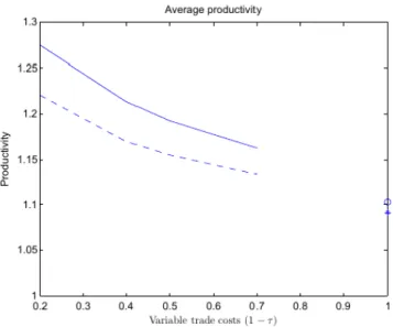
The second graphic shows that, when trade costs are smaller, only more productive firms stay in the market. Tougher competition increases the average productivity in each market. Again, this effect is higher in the comparative advantage industry. The third graphic presents average firm output. We can see that, even with higher trade costs, average firm output is higher in the comparative advantage industry, and it gets higher when trade costs fall. We also can see that comparative advantage firm always produce more, which is explained by the advantage comparative itself and because the average productivity in this industry is also higher, as we have seen in the last graphic.

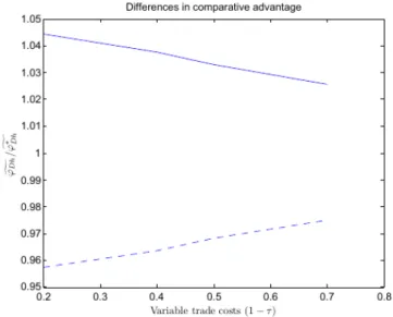
In the next graphic, 𝜙_̃︂𝐷𝑥/ ̃︂𝜙*𝐷𝑥 >𝜙̃︂𝐷𝑦/ ̃︂𝜙

*

𝐷𝑦 is always true. This happens because Domestic

Country has a comparative advantage in industry 𝑥. The graphic also shows that this difference becomes higher when trade costs fall, which means that liberalization magnifies comparative ad-vantages in this economy, as inBernard et al.(2007). The exporting probability rises when trade costs fall. Firms in the comparative advantage industry have higher probability of exporting than firms in the comparative disadvantage industry.

The next two graphics show the mass of domestic firms and the mass of entrant firms re-spectively. The mass of firms producing domestically falls when the economy is opened, ZPC rises and less firms are able to continue producing. However, the mass of firms in comparative advantage industry is higher than in disadvantage industry. Although ZPC is higher in com-parative advantage industry, when we open the economy, the probability of exporting is also higher in this industry. Hence, the expected profit ex-ante in this industry rises more than in

(39)

29

Figure 1.1: Zero-profit and export cut-offs

comparative disadvantage industry and, as consequence, the pool in this industry rises, while in the comparative disadvantage industry, it falls. Thus, the mass of domestic firms is higher in the comparative advantage industry. Analogously, in the comparative advantage industry, when trade costs fall, the mass of entrant firms increases, and in the comparative disadvantage industry it falls.

To analyze welfare gains, we use the logarithmic of the indirect utility of the representative consumer. In the following graphic, liberalization implies welfare gains; note that, when trade costs are lower, indirect utility is higher. We obtain trade gains as in Melitz (2003), since most productive firms export. Thus, they demand more labor, and it increases wages in this market. As consequence, less productive firms stop producing. We also have trade gains, as in

Melitz and Ottaviano (2008). Mark-ups are free to vary, then, when the economy moves from autarky to open economy, competition rises, which induces firms to set lower mark-ups. Thus, less productive firms stop to produce. Furthermore, trade gains are magnified in comparative advantage industry, as in Bernard et al. (2007). Our model incorporates both trade gains discussed above in a unique framework.

Other papers, such as Arkolakis et al. (2019), Edmond et al. (2015), and Edmond et al.

(2018), analyze welfare gains accounting for the impact of procompetitive effects caused by variable mark-ups in trade. The utility function that we use in our paper, the continuous translog expenditure function, has zero procompetitive effects, as emphasized byArkolakis et al.

(40)

30

Figure 1.2: Average productivity

(41)

31

Figure 1.4: Differences in comparative advantage

(42)

32

Figure 1.6: Mass of firms (domestic varieties)

(43)

33

use the indirect utility function to highlight welfare gains when we open the economy.

Figure 1.8: Welfare evaluation

Average mark-up is always constant; to analyze the effect of variable mark-ups, we calculate a weighted average mark-up. It is weighted by the proportion of output of each firm.

\ 𝜇(𝜙𝑟ℎ) = ∫︁ ∞ 𝜙𝑟ℎ 𝜇(𝜙, 𝜙𝐷ℎ) 𝑦𝑟ℎ(𝜙) 𝑌𝑟ℎ 𝑑𝜙.

Where, 𝑌𝑟ℎ is the total output of industry ℎ at market 𝑟.

𝑌𝑟ℎ = 𝑁𝑟ℎ ∫︁ ∞ 𝜙𝑟ℎ 𝑦𝑟ℎ.𝑔(𝜙|𝜙 > 𝜙𝑟ℎ)𝑑𝜙 = 𝑁𝑟ℎ𝛾ℎ𝐼ℎ𝜙𝑟ℎ 𝑤𝛽ℎ 𝑠 𝑤1−𝛽𝑢 ℎ 𝜂1 Where 𝜂1 = 𝑘 ∫︀∞ 1 (𝒲(𝑥𝑒) − 1)/(𝒲(𝑥𝑒)𝑥

𝑘_{)𝑑𝑥 is constant depending on parameter k.}

Calcu-lating \𝜇(𝜙𝑟ℎ); \ 𝜇(𝜙𝑟ℎ) = 𝜂2 𝑁𝑟ℎ𝜂1 . Where 𝜂2 = 𝑘 ∫︀∞ 1 (𝒲(𝑥𝑒) − 1) 2_{/(𝒲(𝑥𝑒)𝑥}𝑘_)𝑑𝑥.

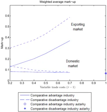
The last graphic shows the weighted average mark-up for both industries, and in domestic and export markets. Firms in the export market set higher mark-ups. In this market, mark-ups fall when trade costs fall, because when trade costs fall, more firms are able to export; thus,

(44)

34

competition gets tougher and firms set lower mark-ups. Note that firms in the comparative disadvantage industry set higher weighted mark-ups than firms in the comparative advantage industry in this market. Competition explains this effect: there are more firms exporting in the comparative advantage industry, and thus competition is tougher. In the comparative disadvan-tage industry, only a few industries are productive enough to sell to the export market.

In the domestic market, the weighted average mark-up is almost constant. There are more firms in the comparative advantage industry, thus, mark-ups in this industry are lower. Ana-lyzing the comparative disadvantage industry, we can see that the weighted average mark-up rises when trade costs fall, and the domestic mass of firms falls when trade costs fall; thus, the weighted average mark-up rises.

Figure 1.9: Weighted average mark-ups

We construct this weighted average mark-up in order to analyze the effects described pre-viously, and find a result that is not found in Bernard et al. (2007) or Melitz and Ottaviano

(2008).

1.6 Conclusion

Our main objective in this paper is to formulate a model that could jointly provide trade gains via two different channels. On one hand, liberalization should shift labor demand up, and thus those firms that were less productive wouldn’t be able to produce after liberalization and would

(45)

35

stop producing. On the other hand, liberalization should make competition “tougher”; thus, mark-ups would get lower and firms that were less productive would stop producing.

We develop a model of comparative advantage that incorporates heterogeneous firms and endogenous mark-ups that respond to the toughness of competition in a market. In such envi-ronment, we accomplished our main objective. We presented several results fromBernard et al.

(2007) and fromMelitz and Ottaviano (2008).

Market size influences firms in a specific industry: larger markets exhibit firms with larger profits and a larger production cutoff. Tougher competition results in lower mark-ups. However, average mark-up is constant. Because of this, we do not observe procompectitive effects in our model. It also causes our model to present a constant measure 𝑁ℎ of available goods in each

sector, although consumer utility exhibits “love of variety”. Thus, when trade costs fall, we observe import substitution in the model.

Trade liberalization raises average industry productivity and average firm output in all sec-tors, because less productive firms stop producing and the most-productive firms export. This effect is higher in the comparative advantage industry, as Bernard et al.(2007) assert, because it provides a new source of welfare gains from trade.

Endogenous mark-ups permit mark-ups to vary when the economy moves from autarky to open economy. It influences every firm individually, by affecting profits, and, as a consequence, determining if the firm will keep producing or not. However, average mark-up does not change, so endogenous mark-ups do not show any result in the industry level. Thus, some results remain identical to those found byBernard et al. (2007). Trade results in gross job creation and gross job destruction in both industries, and the magnitude of these gross job flows varies across countries and industries.

Taking into account welfare gains, our model, as in Bernard et al. (2007), has distinct implications for the distribution of income across factors. In our model it is possible that the real wage of scarce factors also rises with trade liberalization, or, at least, declines less than in Neoclassical models and in what is predicted by the Stolper-Samuelson Theorem.

We also conduct a numerical exercise, where we show many of the theoretical results, as well as how endogenous variables change when trade costs fall. In this numerical exercise we constructed a weighted average mark-up to allow an aggregate markup variable to vary when the economy moves from autarky to an open economy. The result is that when the market has a tougher environment, the weighted average mark-up is smaller.