Unit roots and the welfare gains of cycle smoothing

•

•

' "

#"

G~~li~ V~~a;

EPGE

Escola de Pós-Graduacão em Economia

.;)

Seminários de Pesquisa Econômica I

(2a

parte)

"Ul\TI'rS

BOOTS

AND THFi

WELF ABE GAIBS

OF

CYCLE

SlVIOOTHIl\TG"

LOCAL:

DATA:

HORÁRIO:

\marf.

JOÃO VICTOR ISSLER

(EPGEIFGV)

Fundação Getulio Vargas

Praia de Botafogo, 190 - 10° andar

Auditório

30/05/96 (53 feira)

16:00h

Coordenação: Prof. Pedro Cavalcanti Ferreira Tel: 536-9353

33

g

:~'1

ÁA-•

•

•

---U nit Roots and the Welfare Gains oí Cycle

SInoothing*

Joao Victor Issler and Afonso Arinos de Mello Franco

Graduate School of Econornics - EPGE

Getulio Vargas Foundation

Praia de Botafogo

190 / 1125

Rio de Janeiro, RJ

22253-900

Brazil

May

29,1996

Abstract

li consumption is log-Normal and is decomposed into a linear

deter-ministic trend and a stationary cycle, a surprising result in business-cycle research is that the welfare gains of eliminating uncertainty are relatively small. A possible problem with such calculations is the dichotomy between the trend and the cyclical components of consumption. In this paper, we abandon this dichotomy in two ways. First, we decompose consumption into a deterministic trend, a stochastic trend, and a stationary cyclical com-ponent, calculating the welfare gains of cycle smoothing. Calculations are carried forward only after a careful discussion of the limitations of macroe-conomic policy. Second, still under the stochastic-trend model, we incorpo-rate a variable slope for consumption depending negatively on the overall volatility in the economy. Results are obtained for a variety of preference parameterizations, parameter values, and different macroeconomic-policy We gratefully acknowlwdge the comments of Pedro C. Ferreira and Samuel Pessoa, who are not responsible for any remaining errors in this paper. Osmani T. Guillen provided excellent research assistance. We thank CNPq-Brazil for financiai support .

•

goals. They show that, once the dichotomy in the decomposition in con-sumption is abandoned, the welfare gains of cycle smoothing may be sub-stantial, especially due to the volatility effect.

1.

Introduction

A main question of economics is whether governrnents should or should not inter-vene in markets. Although there are several aspects of this issue, a particularly important one for macroeconomists is the welfare gains of cycle smoothing. The idea is straightforward. The best a macronomist can hope to achieve in terms of welfare improvement is eliminating completely the variance of transitory

com-ponents of macroeconomic aggregates. In some sense, this is the equivalent of

eliminating systematic risk, even if idiosyncratic risk is still present. Assuming a complete success in this task, Lucas(1987, 3) calculates the amount of extra con-sumption a rational consumer would request in order to be indifferent between an infinite sequence of consumption under uncertainty and a cycle free sequence. For 1983 figures, using a reasonable parametric utility function, the extra con-sumption is about $ 8.50 a person, a surprisingly low amount. This led to the conclusion that cycle smoothing is undesirable, since the upper bound of its payoff is extremely low, while the costs of implementing such policy may be very high.

The power of the argument comes from the simplicity of the calculations. In

order carry it forward though, several simplifying assumptions were made. In

particular, it is assumed that consumption is log-Normally distributed about a

deterministic trend, that individuals are not constrained to borrow against future income, and that there is perfect insurance against individual income risk.

Imrohoroglu(1989) and Atkeson and Phelan(1995) recalculate the welfare gains of counter-cyclical policy relaxing respectively the last two assumptions above. Both papers are concerned with the lack of complete markets in real economies, which could invalidate earlier calculations. Here, we turn our attention to the

first assumption, that consumption is log-Normal about a deterministic trend,

assuming instead, that it is log-Normal about a stochastic trend. Moreover, we

also consider the effects of volatility on growth with the recent estimates of Ramey and Ramey(1995) using panel data.

At first, the assumption that consumption is log-Normal about a

determin-istic trend may seem innocuous, but in fact it is noto When (log) consumption is decomposed into a (deterministic linear) trend and a (stochastic) cycle, this decomposition embeds the dichotomy that random shocks can only affect the

be-•

•

havior of the cycle, but not the behavior of the trend. The cycle, however, has a

bounded variance. If the trend is not deterministic, it usually has an unbounded

asymptotic variance. Since the consumer is assumed to be risk averse, he/she dislikes having an ever increasing variance of consumption, which would be the case in the in the presence of a stochastic trend .

There are several ways in which a trend can be stochastic. Here, we follow

the substantial literature in macroeconometrics, after the work of Beveridge and Nelson(1981), and Nelson and Plosser(1982), and assume that the consumption trend evolves as a random walk. In this case, its variance is O(t), i.e., it must be

divided by t - the time index - to be bounded. Using the model with a unit-root

trend, we recalculate the welfare gains of cycle smoothing, after some discussion on the limits of counter-cyclical policies.

A negative relationship between growth and volatility has always been a styl-ized fact in the growth literature. Although the link between the two is not yet fully understood. Ramey and Ramey(1995) provide strong evidence that such re-lationship do existo Their result is robust to changes in the conditioning set, and in the specification of the mo dei , and (again) challenge the dichotomy between the growth and the cyclical component of economic aggregates. Here, we use their estimates on the negative relationship between growth and volatility to recalculate the welfare gains of cycle smoothing.

The two exercises implemented in this paper can be thought of as a relaxation of the usual dichotomy between trend and cycle embedded in the traditional linear trend model for macroeconomic aggregates. Considering unit roots relax the assumption that the trend is deterministic. Thus, the slope of consumption has a stochastic component. In this case, counter-cyclical policy may be a way of controlling this component, thus having a greater impact on welfare then in the deterministic trend case. Allowing a volatility effect on growth, such as the one found in Ramey and Ramey(1995), and assuming that growth is the same for macroeconomic aggregates, makes this variable slope a function of the volatility in the economy. Here, counter-cyclical policy affects directly the average growth rate of the economy, as it works towards the reduction of economic volatility.

The paper is divided as follows: Section 2 provides a theoretical and statistical framework to evaluate the welfare gains of cycle smoothing. Section 3 provides the estimates that are used in calculating these welfare gains. Section 4 provides the calculations results, and Section 5 concludes. There is also an Appendix providing the econometric background necessary to implement the calculations carried out in the paper.

•

2. The Problem

Lucas(1987) proposed the folIowing way to evaluate the welfare gains of cycle

smoothing. Suppose that consumption

(Ct)

is log-Normally distributed about a

deterministic trend:

(2.1) where log(Zt) f"V N(O,

CTn.

Cycle-free consumption wilI be the sequence {c;}~,

where c;

=

E(ct)

=

ao(1

+

ad

t

exp(CT~/2). ~otice that {c;}~o is the resulting sequence when we replace the random variable Ct with its unconditional mean.

Risk averse consumers prefer {c;}~ to {Ct}~, since the former is deterministic

and they dislike risk. Then, to evaluate the welfare gains of cycle smoothing

amounts to calculating À, that solves the following equation1:

E

(Eo

I:,et

U

((1

+

À)Cd)

=

I:,etu(c;),

t=O t=O

(2.2)

where

Et{-}

=

E(.

I f2t) is the conditional expectation operator of a random

variable using f2t as the information set. Then, the welfare gains are expressed

as the compensation À, that consumers would require at ali dates and states of

nature, that makes them indifferent between the uncertain stream {Ct}~o and the

stream {c;}~o. Although the solution to the problem is simple and ingenious,

this is not without a cost. Notice that a lot of structure is imposed in solving

it. First, it is assumed that {Ct}~o is log-Normal and trend-stationary. Second,

a parametric utility function is chosen in order to calculate (2.2). Although the latter is a standard procedure in the literature, the former are noto Assuming

log-Normality alIows the mean of consumption to be expressed explicitly in terms

of CT~. Thus, it is used for the sake of analytic simplicity. Trend-stationarity, on the other hand, has two implications: (i) one has not to deal with the conditional

expectation of the sequence {u(c;)}~, and

(ii)

the random variable Ct has a

bounded variance. The second is critical for the proposed problem, since otherwise the left hand side of (2.2) may not be defined.

Here, instead of assuming log-Normality and trend-stationarity of {Ct}~, we

first test for them. Tests results confirm the former but not the latter. Instead of trend-stationarity, unit-root tests performed here and elsewhere show evidence

that {cd~o is difference-stationary. Despite the well known power problems of

1 Notice that Lucas(1987) uses the unconditional mean operator instead of the conditional

mean operator in (2.2). The same problem can be proposed using the conditional expectation instead. This is exactly how we proceed in this paper .

•

•

unit-root tests against local altematives, and the observation-equivalence between trend-stationarity and difference stationarity, it seems reasonable to examine how the results for>. in (2.2) would change if trend-stationarity is abandoned.

To start the discussion of difference-stationary consumption, we first assume that the utility function is in the CES class:

(2.3)

where

u(Ct)

approaches ln(Ct) when

a

~ 1. As shown in Beveridge and

Nel-son(1981), every linear difference-stationary process can be decomposed as the sum of a deterministic term, a random walk trend, and a stationary cycle (ARMA process). We apply this result to ln(Ct), i.e.,

t t - l

ln ao

+

ln(l

+

aI) . t

+

L

ti

+

L

'l/Jj!-Lt-j

i=l j=O

- ln[ao(l

+

at}t]

+

In(Xt}

+

ln(yt),

(2.4)

(2.5)

where, ln[ao(l + at}t] is the deterministic term, In(Xt ) = L~=l ti is the random

walk component, and In(Yt)

=

L~~ 'l/Jj!-Lt-j is the M A(

00)

representation of the

stationary part (cycle). The permanent shock (tt) and the transitory shock

(J-Lt)

are assumed to have a bi-variate Normal distribution as follows:

(2.6) i.e., shocks are independent, thus uncorrelated. across time, but may be

contem-poraneously correlated if a12

=I

O. This structure certainly implies

conditionallog-Normality for

XtYt,

although the converse may not be true. Under normality, the structure in (2.6) encompasses several cases of trend-cycle decomposition meth-ods existent in the literature, particularly those based on the Beveridge-Nelson decomposition. For example, the Unobserved Components method discussed by

Watson(1986), and the method in King et Al.(1991) impose a12 = O. However,

for the method proposed by Vahid and Engle(1993) a12

=I

O, in general.

Under (2.3), (2.4) and (2.6) we can re-calculate (2.2). Its left-hand side is given by:

•

00

1

00

[(1

CT)2 W2]

EoL,6tu((l

+

A)ct) = ~ (1-

A)l-U

_L

,6t exp - 2 . t . ao(l

+al)t,

t=O 1 CT t=o

(2.7)

t - l t - l

where

w;

= (CTu • t

+

2 . CT12

L

'l/Jj

+

CT22

L

'l/JJ).

Notice that although the Ct

j=O j=O

has an unbounded conditional asymptotic variance, the expression (2.7) is weli defined. The reason is simple: the utility function in (2.3) above is homogeneous of degree (1 - CT) in Ct. Thus, ,6tu((l

+

A)Ct) = ,6utu((l

+

A),6tCt ). The random variable Ct is Op(t3/2) , thus, t-3/2Ct is Op(l), and so is u((l

+

A)r3/2Ct). Since

l/,6t is of Order higher than

tl/

2_{, ,6utu( (1}

₊

_{A),6tct ) converges in probability, and}

Eo L~ ,6tu( (1

+

A)Ct) is defined.

Calculating the right-hand side of (2.2) for the difference-stationary case re-quires first some discussion about the limitations of macroeconomic policy. Im-plicit in (2.2) is the idea that the policymaker can deliver to the consumer the

sequence {c;}~o instead of {cd~. Notice that {c;}~o can be free of any trend

variation, cyclical variation, or both. In the exercise proposed in Lucas(1987), c; = ao(l

+

adt

E(Zt).

There, ali the cyclical variation in Ct is eliminated. Since the trend is deterministic, this is equivalent to eliminating all the

vari-ability in Ct itself. Here, this equivalence is lost. We thus consider in this pa-per two possibilities. In the first, the policymaker has full power, i.e., he/she controls both the variance of the trend and the variance of the cycle. Then,

c; = ao(1

+

adt Eo(ct)

=

ao(1

+

adt exp

[~].

In the second case, the

policy-maker has only the ability to control the cyclical variability of Ct. Of course, this

poses no problem when CT12 = 0, since the variance of the trend innovation is

unaffected when the variance of the cyclical innovation goes to zero. However, this is not the case when CT12

i-

O. To deal with this case, consider the following

decomposition:

(2.8) where we decompose Et into two orthogonal components: J..Lt and

l/t,

where

l/t

rv

N(O,

CT;).

In

this case, controlling the variance of the cyclical innovation

(j.Lt),

replaces the sequence

{Ed

~ by

{l/d

~o.

It is easy now to calculate the right-hand side of (2.2). In the case where the

•

In the case where the policymaker has limited power, it is:

[

t-l [

00 1 00 (1 - 0") (1 - 0") O"~ • t

+

0"22 L:

'ljJJ

EOLj3t

u(c;)

= - - Lj3t

exp

---~--2---...:.j-=O_..L.... x (00(1 +ol)t)l-U.

t=O 1 - O" t=0

(2.10)

Given the parameters defining the processes {c;}~o and {Ct}~o, the

compen-sation À can now be solved as a function of (O", j3) for the two cases (policymaker with full and limited power). The two solutions are respectively:

(2.11)

and:

À = ) = 0 _

1

[

L:~oj3texp

(1;u) (1-0")

O"~

t + 0"22

~tl

'ljJJ

(1 + Odt<l_U)]

~

L::oj3t exp [(l-utw~]

.

((1 + ot)t)l-U .

(2.12)

The same results for À can be derived. under log-utility. If the cycle is an AR(I)

process, with autoregressive coefficient cp (which is exactly what we get below), the expressions simplify to the following: if the policymaker has full power, we have:

À = exp

[~

(1

~1{3

+

1

~2~{3

+

1

~~(3)]-

L

(2.13)

In the case where the policymaker has limited power, we get:

(2.14)

Expressions (2.13) and (2.14) help to shed some light on comparative statics. They show that

>.

is an increasing function of

f3,

i.e., the risk compensation in-creases the less the consumer discounts the future. This result is intuitive, since under unit-roots, the consumer gets a monotonic increase in risk as the planning horizon increases. Moreover, an increase in risk. represented by an increase in either CTu, CT22, or CT12 would also increase

>..

since risk averse consumers dislike

risk.

3.

The

Data and Estimates

The data used in this paper are extracted from CITIBASE. They are post-war quarterly consumption, investment, and private GNP in constant 1987 dollars.

Private GNP is the difference between GNP and governrnent purchases. Ali data

are expressed in per-capita terms. This is the same data set used in King et

Al.(1991) and Issler and Vahid(1995), spanning from 1947:1 to 1988:42

• The choice

of data reflects the idea of performing a trend-cycle decomposition based on a the-oretical model. One possibility is to use the model of exogenous growth discussed in King, Plosser and Rebelo(1988), where consumption, investment and output share a common trend given by the random walk technology processo Equiva-lently, we could use Romer's(1986) endogenous growth model, which delivers the same long-run implications.

Figure 1 shows the three series in log-levels. Using data from 1947:1 to

1988:4, the cointegration tests performed in either King et Al.(1991) or Issler and Vahid(1995) do not reject the null that the so called great-ratios are the cointegrating linear combinations, and that these three series share a common stochastic trend. This common trend can be interpreted either as the productiv-ity random walk process (King, Plosser and Rebelo) or as the long-run physical capital stock (Romer). The Common-cycles test performed in Issler and Vahid, indicate that the three series share two common cycles, which can be interpreted as the trasitional dynamics of the system.

Based on cointegration and on common-cycles test results, we perform the trend-cycle decomposition using the method proposed by Vahid and Engle(1993), and applied in Issler and Vahid(1995). Besides imposing tested common-trend restrictions, it also imposes tested common-cycles restriction in the identification

2We use this reduced data span so as to match the sample used in King et a\.(1991) and IssIer and Vahid(1995). In doing so we avoid re-estimating the parameters used here.

•

of trends and cycles3_{. The Appendix discusses in some length how to decompose}

a multivariate data set containing unit roots into trends and cycles using the method in Vahid and Engle.

The results for consumption of applying this multivariate decomposition method, are presented in Figure 2. Table 1 shows the results of the variance decomposition of the one-step-ahead innovation of consumption. Cyclical shocks to consumption do not seem to be very important, a result consistent with consumption smooth-ing and in line with the evidence of the empirical consumption literature worksmooth-ing with aggregate data.

Tests of normality for (log) consumption reveal that indeed this is a reason-able assumption. In Treason-able 1, the results of the Jarque and Bera(1987) Lagrange

Multiplier show that normality cannot be rejected for In(XtYt) at usual

signif-icance leveIs. For individual components, we find that both _{In(Xt )} and In(Yt)

are normal at 1 % significance, although ln(Yt) is not at 5%. At any rate, they

are borderline cases. Having In(XtYt) normally distributed validates the use of

the convenient hypothesis that non-deterministic consumption has a log-Normal distribution, implicit in deriving (2.11), (2.12), (2.13), and (2.14).

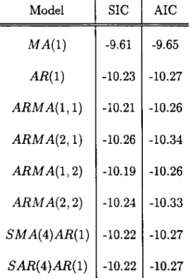
The next step for calculating À is to estimate the cyclical process In(Yt) =

L~-==Õ 'l/JjJ.Lt-j, in particular the sequence {'l/Jj }~. This is accomplished by

esti-mating severallow-order ARM A(p, q) processes, and then selecting among them

the one with the lowest Schwarz Information Criterium (SIC). The results from

this estimation are presented in Table 2. The best model is the AR(l):

ln(Yt) = 4> ln(Yt-d

+

J.Lt· (3.1)

Notice that although the ARM A(2, 1) and the ARM A(2, 2,) specifications have

smaller information criteria, they show signs of common factors, a very common

finding for ARMA estimation. Thus, the AR(l) specification is preferred.

Inspec-tion of the Q-statistic and other diagnostic tests show that (3.1) is a reasonable

representation of the data. A particularly interesting result attached to the AR(l)

process is that L~-==Õ

'l/Jj

and L~-==Õ

'l/JJ

can be easily calculated. Since

'l/Jj

=

q),

we have:

L~~

'l/Jj

=

\-=-~

and

L~~

'l/JJ

=

;--::.~;t.

The estimated autoregressive

coeffi-3The method in King et al.(1991), which imposes tested cointegration restrictions, is just-identified. Thus, the method in Vahid and Engle(1993) imposes over-idetifying restrictions on the reduced form of the data to recover trends and cycles. 80th decompositions are in fact based

on the multivariate version on the 8everidge and Nelson(1981) trend-cycle decomposition, where trends are random walks (or martingales) and can be interpreted as the value that the long-run forecast of the original series converges to.

ti

cient is 0.86, which shows that although the cycle is not a long-memory process, it certainly has persistency features.

The only issue left to discuss is the variance of innovations to trend and to cycle and the deterministic components of ln(ct). The innovations to trend were obtained by simply first differencing it. Since the trend is a Martingale with respect to the information set in the VECM in (6.7) below, its first differences

are its innovations. The cyclical innovations were estimated through the AR(I)

estimation discussed above. Trend and cycle innovations are negatively correlated, as shown in Table 1. The variance of the trend innovation is much bigger than its cyclical counterpart. The results of the orthogonalization procedure described

in (2.8) above are also shown in Table 1. The deterministic components were

extracted from the data by simply detrending the stochastic trend component and demeaning the cyclical component. The deterministic parts were then added

together, and the estimates of the coefRcients ao and aI determined. The results

are reported in Table 1 as weli.

4. The Calculation Results

Given the estimates of CTn, CT22, CT12, CT~, ao, aI, and

'l/Jj

found above, we can calculate >.({3, CT), i.e., the value of the compensation the consumer requires at ali dates and states to be indifferent between {(I

+

>.)Ct}~ under uncertainty and

{

c;}~. Table 3 displays some values of this function for selected values of ({3, CT). The range of values is from 0.0064% to 0.66% in the case where the policymaker

has limited power, and from 0.26% to 0.85% in the case the policymaker has full

power. These results, compared to the appropriate ones found in Lucas(1987), show that considering unit roots increase the welfare gains of cycle smoothing. For example, using {3 = 0.95 in an annual basis, Lucas found >.'s of 0.008%, 0.042%,

0.084%, and 0.17% for the following values of CT respectively: 1,5, 10, 20; see Table

3 (c). Compared to the values reported in Table 3 (a) and (b), these numbers

are much smaller. For the full power case, our number is 32.5 times larger under

log-utility. For CT = 20, it is 3.7 times larger. Even if we compare Lucas findings to the case where the policymaker has limited power, we find large discrepancies: for CT

=

5, our number is 9.9 times larger; for CT

=

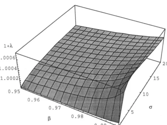
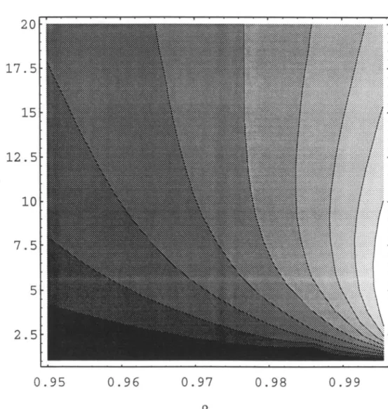
10, it is 6.3 times larger; and

for CT = 20, it is 3.5 times larger. Figures 3 through 12 show different aspects of the impact of the function >.({3, CT). Clearly, a decrease in the rate of discount for future utilities increases >. exponentialiy, since it discounts less long-run utilities with very large variances. The effect of an increase in risk aversion also increases

•

•

À for the full power case, although a rebound is found for the limited power case. The discrepancies found between our results and those in Lucas are no surprise.

If the trend in consumption is stochastic, the consumer faces unbounded

uncer-tainty asymptotically. This, of course, he/she dislikes more than the bounded uncertainty implicit in the calculations in Lucas. Therefore, under unit-roots, consumption compensation must be higher. In this case, it is at most 32.5 times higher. For 1994 figures, the maximum total compensation per capita, in dollars of 1987, for the values of (3 and a considered in Table 3 (a) and (b) is $ 116.73. Of course, this is much larger than the benchmark value of $ 8.50 given in Lucas. Although this amount is far from being negligible, it is also not large either. In some sense, this results illustrates the price in terms of welfare of the unit-roots debate, e.g. Christiano and Eichenbaum(1989) and Campbell and Perron(1991). Given the fact that the consumer discounts the future exponentially, even the uncertainty of the conditional mean of consumption under a unit-root is negligible asymptotically. Thus, although the "asymptotics are different " for hypothesis testing, as Stock and Watson(1988) put it, it is not very different in terms of welfare implications.

We now tum to the connection between cycle smoothing and growth. Ramey and Ramey(1995) found strong evidence that the variance of the innovations to growth has a negative effect on growth, controlling for a reasonable set of

vari-ables. This result is robust to changes in the specification of the variance to the innovations and to changes in the controlling variables. A similar relationship between volatility and growth was also found by other authors, e.g., Kormendi

and Meguirre(1985) and Grier and Tullock(1989) inter-alia. Ramey and Ramey

note that if this relationship is true, calculations such as Lucas(1987) are invalido

The problem lies in using the same growth rate of consumption for {Ct}~ and

{c;}~o, when different rates should be used due to the positive effect on growth

resulting from cycle smoothing.

To investigate this issue numerically, we considered the effect found by Ramey and Ramey in our calculations. For the OECD-country sample, they found a negative slope of 0.385 for the volatility of growth in the growth equation. This means that if alI innovation volatility (standard deviation) is controlIed, growth

should increase by 0.385 X ai a year, where ai is the standard deviation of the total

innovation to growth. For the US, Ramey and Ramey estimate of ai is 0.0244.

Thus, under their estimates, controlling all the innovation to growth would imply an increase to growth in the US of 0.94% a year, which is a sizable effect. We incorporate this effect in our calculations assuming that income and consumption

growth will be identical under the effects of cycle-smoothing. This hypothesis can be based on either the exogenous or endogenous growth models discussed

above, and is true at least in steady-state. Having the policymaker controliing ali

the variance of the innovations to the system corresponds to the full power case discussed above. In the case of limited power, we assume that the policymaker controls the same proportion of the total innovation growth variance as he/she does for the total innovation to consumption variance. Thus, growth will increase

by [(0.0000596)1/2 x (1- (1- 0.131746031)1/2)] x 0.385 = 0.0641001% a year,

which is a much smalier effect. Results are presented in Table 3 (d) and (e). Incorporating the interaction between growth and volatility under unit roots completely changes the order of magnitude of the compensation the consumer requires to accept risk. For the full power case the compensation can be as great as 40%! Even for the case of limited power it can be as high as 3.5%. We do not suggest here that these are the best estimates for the welfare gains of cycle smoothing, given how precariously we estimated the effects on growth of controlling volatility. However, these number illustrate that once the dichotomy between the growth and the cyclical component is relaxed, the welfare gains of cycle smoothing can be substantial.

5.

Conclusions

Our results show that once the dichotomy between trend and cyclical components of consumption is lost, calculations of the welfare gains of cycle smoothing may be greatly altered. By itself, the assumption that consumption has a unit root

cannot change dramatically the value of consumer's compensation À, although À

can increase more than 30 fold. However, the impact of controlling volatility can be substantial, as the results in Table 3 (d) and (e) show. Although our results are still preliminary, they show a direction to which counter-cyclical policy can matter for a rational consumer. However, further research is needed to investigate how robust our results are to changes in the decomposition method used.

References

[1] Atkeson, A. and Phelan, C.(1995), Reconsidering the Cost of Business Cycles

with Incomplete Markets, NBER Macroeconomics Annual, pp. 187-207, with

•

•

[2] Beveridge, S. and Nelson, C.R(1981), ., A new Approach to Decomposition of Econonllc Time Series into a Permanent and Transitory Components with Particular Attention to Measurement of the "Business Cycle" ," Journal of Monetary Economics, voI. 7, pp. 151-174.

[3] Campbell. J.Y. and Perron, Pierre. Pitfalls and Opportunities: What

Macroecononllsts Should Know about Unit Roots. NBER Macroeconomics

Annual, 1991.

[4] Christiano, Lawrence J., and Eichenbaum, Martin (1989). Unit Roots in

GNP: Do We Know and Do We Care? Carnegie-Rochester Conference Series

on Public Policy.

[5] Engle, RF. and Granger, C.W.J.(1987), "Cointegration and Error Correc-tion: Representation, Estimation and Testing," Econometrica, voI. 55, pp. 251-276.

[6] Grier, Kevin B. and Gordon Tullock. "An Empirical Analysis Of

Cross-National Econonllc Growth, 1951- 80," Journal of Monetary Economics,

1989, v24(2), 259-276.

[7] lssler, J.V. and Vahid, F.(1995), "Common Cycles in Macroecononllc Ag-gregates," Working Paper: Graduate School of Econonllcs - EPGE, Getulio Vargas Foundation, Rio de Janeiro.

[8] lrnrohoroglu, Ayse. "Cost Of Business Cycles With Indivisibilities And

Liq-uidity Constraints," Journal of Political Economy, 1989, v97(6), 1364-1383.

[9] Jarque, Carlos M. and Bera, Anil K. (1987), A Test of Normality of

Ob-servations and Regression ResiduaIs. International Statistical Review, 55, 2,

163-172.

[10]

[11]

King, RG., Plosser, C.I. and Rebelo, S.(1988), "Production, Growth and

Business Cycles. lI. New Directions," Journal of Monetary Economics, voI.

21, pp. 309-341.

King, RG., Plosser, C.L, Stock, J.H. and Watson, M.W.(1991), "Stochastic

Trends and Econonllc Fluctuations," American Economic Review, voI. 81,

pp. 819-840.

[12] Kormendi, Roger and Meguire. Phillip(1985), Macroeconomic Determinants of Growth: Cross Country Evidence.ournal of monetary economics, voI. 16, pp. 141-163.

[13] Lucas. Robert(1987) , Models Df Business Cycles. Oxford: Blackwell.

[14] Nelson, C.R. and Plosser, C.L(1982), "Trends and Random Walks in

Macroe-conomic Time Series," Journal Df Monetary Economics, voI. 10, pp. 139-162.

[15] Ramey, Garey, and Ramey, Valerie, A.(1995), Cross-Country Evidence on

the Link Between Volatility and Growth, American Economic Review, voI.

85, 5, pp. 1138-1150.

[16] Romer, P.(1986), "Increasing Returns and Long Run Growth", Journal Df Political Economics. voI. 94, pp. 1002-1037.

[17] Romer, P.(1989), "Capital Accumulation in the Theory of Long-Run Growth," in R. J. Barro (ed.) " Modern Business Cycle Theory," C amb ridge ,

MA: Harvard University Press.

[18] Romer, P.(1987), "Crazy Explanations for The Productivity Slowdown,"

NBER Macroeconomics Annual, voI. 1, pp. 163-201.

[19] Stock, J.H. and Watson, M.W.(1988), "Testingfor Common Trends," Joumal

Df the American Statistical Association, voI. 83, pp. 1097-1107.

[20] Stock, J.H. and Watson, M.W.(1988), "Variable Trends in Economic Time Series," Journal Df Economic Perspectives, voI. 2, 3, pp. 147-174.

[21] Vahid, F. and Engle, R.F.(1993), "Common Trends and Common Cycles,"

Journal Df Applied Econometrics, voI. 8, pp. 341-360.

[22] Watson, M.W.(1986), "Univariate Detrending Methods with Stochastic Trends," Journal Df Monetary Economics, voI. 18, pp. 49-75.

6. Appendix

6.1. Co-Movement Restrictions in Dynamic Models

Before discussing the dynamic representation of the data, and the trend-cycle decomposition method used, we present the definitions of common trends and

•

•

common cycles; for a full discussion see Engle and Granger(1987) and Vahid and Engle(1993) respectively. First, we assume that

Yt

is a n-vector of 1(1) variables, with the following stationary Wold representation (MA( 00)):

(6.1) where

C(L)

is a matrix polynomial in the lag operator,

L,

with

C(O)

=

In,

and

00

L

j

ICjl

<

00,

Et

is a n x 1 vector of stationary one-step-ahead linear forecast j=O

errors in

Yt,

given information on lagged values of

Yt.

We can rewrite equation (6.1) as:

ô.Yt

=

[C(l)

+

Ô.C*(L)jEt.

(6.2) If we integrate both sides of equation (6.2) we get:

00

Yt -

C(l)L Et-s+ C*(L)Et

(6.3)

s=O - Tt

+

Ct ·

Equation (6.3) is the multivariate version of the Beveridge-Nelson trend-cycle representation (Beveridge and Nelson(1981)). Series

Yt

are represented as sum of a random walk part Tt , which is called the "trend," and a stationary part Ct ,

which is called the "cycle."

Definition 1: The variables in

Yt

are said to have common trends (or cointe-grate) if there are r linearly independent vectors, r

<

n, stacked in a r x n matrix a', with the property that:

a'

C(l)

=

O.

rxn

(6.4)

Definition 2: The variables in

Yt

are said to have common cycles if there are s linearly independent vectors, s ::::; n - r, stacked in a s x n matrix

a',

with the property that:

a

I

C*(L)

= O.

sxn (6.5)

Thus, cointegration and common cydes represent restrictions on the elements of

C(l)

and

C*(L)

respectively. We now discuss restrictions to the dynamic autoregressive representation of economic time series arising from cointegration

•

(common trends) and common cycles. First. we assume that Yt is generated by a

Vector Autoregression (VAR):

Yt = r1Yt-l

+

r 2Yt-2

+ ... +

rpYt-p

+

Et, (6.6)

Engle and Granger(1987) show that, if and only if the elements of Yt

coin-tegrate, the system (6.6) can be written as a Vector Error-Correction Model (VECM). This shows the existence of cross-equation restrictions in the VAR given by cointegration:

D..Yt = riD..Yt-l

+

r;D..Yt-2

+ ... +

r;_lD..Yt-P+1

+

'Ya'Yt-l

+

êt, (6.7) where 'Y and a are full rank matrices of order n x r, r is the rank of the cointegrating

space, 1 - L:f=l ri = -'Ya', and r; = - L:f=j+1 ri' Given the cointegrating vectors

stacked in a', they show that (6.7) parsimoniously encompasses (6.6). Clearly,

given the parameters in (6.7), one can recover those of (6.6) by the formulae

above. Moreover, (6.6) has n2 _{x p parameters in the conditional mean, while (6.7)}

has n2 x (p - 1)

+

n· r. Thus, n x (n - r) fewer parameters.

Vahid and Engle(1993) show that the dynamic representation of the data Yt

may have additional cross-equation restrictions if there are common cycles. To see

this, recall that the cofeature vectors ã~, stacked in an

s x n

matrix

ã',

eliminate all the serial correlation in D..Yt. Now, rotate ã to have an s dimensional identity sub-matrix as follows:

-, - [1 -. ']

a - s a , (6.8)

thus, ã· 'D..Yt can be looked at as s pseudo-structural form equations for the first

s elements of D..Yt. Complete the system by adding the unconstrained VECM

equations in (6.7) for the remaining n - s elements of D..Yt to get the following

system: [ 1 -.,

1

ô

~-s

D..Yt =

u.

r··

2

r··

p-l

J.]

(6.9) D..Yt-P+l

_,

a Yt-l

where

r;-

and 'Y. represent the partitions of

r:

and 'Y respectively, corresponding

•

..

• [ I -.,

1

7Jt =

Ô

~-s

€t·

It is easy to show that (6.9) parsimoniouslyencompasses (6.7). Since

[~ f·-~

1

is invertible, it is possible to recover (6.9) from (6.7) by inverting it. Notice, how-ever, that the latter has

s

x

(n .

p

+

r) - s

x

(n - s)

fewer parameters.

6.2. The Trend-Cycle Decomposition Method (Vahid and Engle(1993»

We now discuss the trend-cycle decomposition proposed in Vahid and Engle(1993). Recall equation (6.3):

00

Yt =

C(l) L€t-s

+

C*(L)€t.

(6.10)

s=O

Consider now the following special case: n = r

+

s. Stack the cofeature and

the cointegrating combinations:

[ ã'Yt _a'Yt

1

= [

_a'Ct ã'1't

l.

(6.11)

The n x n matrix

A

= [

~:

1

has full rank, and therefore is invertible. Partition

the columns of the inverse conformably to A as A-I

=

[ã-

a-],

and recover the

common-trend common-cycle decomposition by pre-multiplying the cofeature and

cointegrating combinations by A-I:

(6.12) implying _Tt

=

ã- (ã'Yt) and

C

t

=

a- (a'Yt).

Notice that the first term in (6.12) loads into the cofeature-vector linear combi-nations, while the second loads into the cointegrating-vector linear combinations. lndeed, this illustrates that the first are trend generators, while the second are cycle generators in this decomposition .

Tablel: Descriptive Statistics Df the Elements Df ln( Ct)

Component Estimate Jarque-Bera Statistic P-value

ln(XtYt) 4.34 0.11 ln(Xt) 5.54 0.063 ln(Yt) 6.43 0.04 ao 6.798 aI 0.00443 (T11 6.39E-5 (T22 3.51E-5 (T12 -1.80E-5 a2 v 5.47E-5 cP 0.86

..

Table 2: Cyclical Component Estimation Using ARMA Models Model

_I

SlC

_I

AlC MA(l) -9.61 -9.65 AR(l) -10.23 -10.27 ARMA(l,l) -10.21 -10.26 ARMA(2,1) -10.26 -10.34 ARMA(1,2) -10.19 -10.26 ARMA(2,2) -10.24 -10.33 SMA(4)AR(1) -10.22 -10.27 SAR(4)AR(1) -10.22 -10.27 •

Table 3: Consumption Compensation (,X%) for Different

(/3,

(J) Values (a) Policymaker with Full-Power

/3

Equivalent in a Yearly Basis (J = 1 (J = 5 (J = 10

/3

= 0.950 0.26 0.51 0.58

/3

= 0.971 0.42 0.61 0.64

/3

= 0.985 0.85 0.72 0.70

(b) Policymaker with Limited-Power

/3

Equivalent in a Yearly Basis (J

=

1 (J = 5 (J = 10

/3

= 0.950 0.0064 0.414 0.53

/3

= 0.971 0.0066 0.497 0.58

/3

= 0.985 0.0066 0.586 0.64

(c)

Lucas(198'l) Benchmark Values

(J = 20 0.62 0.66 0.69 (J = 20 0.60 0.63 0.66

/3

Equivalent in a Yearly Basis (J = 1 (J

=

5 (J

=

10 (J

=

20

/3

= 0.950 0.008 0.042 0.08 0.17 ( d) Volatility Effect: Policymaker with Full-Power

/3

Equivalent in a Yearly Basis (J = 1 (J

=

5 (J

=

10 (J

=

20

/3

= 0.950 20.7 7.3 4.2 2.5

/3

= 0.971 36.3 8.6 4.6 2.6

/3

= 0.973 40.6 8.8 4.7 2.6

(e) Volatility Effect: Policymaker with Limited-Power

/3

Equivalent in a Yearly Basis (J

=

1 (J

=

5 (J

=

10 (J

=

20

/3

= 0.950 1.3 0.580 0.362 0.223

/3

= 0.971 2.2 0.695 0.403 0.238

..

Figure 1: Private Output, Consumption and Fixed Investment per-capita

3.0-. - - - .

2.5

~~~-~--.-~-'~~~-~-~-~

/---~---I - - __

/~--./~_/-~

~

J

2.0

CJ) C>

1.5

o

c

1.0

~

/~,

I-~"

~

," ,_,o, .' ' ."

,--~'

----.' ,__ ,o, v , . ' \ / " . , ' ' • , __ ,_.. _. ,'- r ' ' " ' :

O 5

• . '

.. '..

, "

,

, , "

.

.

-00 ,

• i ,

,

50

55

6065

70

75

80

85

90

•

Figure 2: Consumption and its Components

2.8 2.8 2.6 2.6 2.4 2.4 2.2 2.2 2.0 2.0 1.8 1.8 50 55 60 65 70 75 80 85 90 50 55 60 65 70 75 80 85 90

- Consumption per-capita - Deterministic Linear Trend

0.03 0.08 0.02

I

,

N\

A",

{nA.

0.04 0.01 0.00

I1

\f

I

~I

V\I \

flf

If

~

I

I

I I

\J

0.00 -0.01

:::I""""""""""""",~"",~""",

.I

-0.04 -0.08 50 55 60 65 70 75 80 85 90 50 5"5 ₆₀ 65 70 75 80 85 90

. _ - - - -

_.~---Figure 3: Compensation as a Fuction of the Discount Rate and Relative Risk A version Coetlicient

Policymaker with FuIl Power

1. 006 1. 00

Figure 4: Contour Map for the Discount Rate and Relative Risk A version Coefticient Policymaker with Full Power

20 17.5 15 12.5 10 7.5 5 0.95 0.96 0.97

13

0.98 0.99

li

•

Figure 5: Compensation as a Function of the Relative Risk A version Coefficient J3=O.987, Equivalent to 0.95 in a Yearly Basis

Policymaker with Full Power

1+À. 1. 006 1. 0055 1. 005 1. 0045 1. 004 1.0035 cr 15 20 1. 0025

• 1+À. 1. 007 1. 006 1. 005 1.004 1. 003 1.002

Figure 6: Compensation as a Function of the Discount Rate 0=1.1

Policymaker with Full Power

Figure 7: Compensation as a Fuction of the Discount Rate and Relative Risk A version Coeflicient

Figure 8: Contour Map for the Discount Rate and Relative Risk A version Coefficient Policymaker with Limited Power

20 17.5 15 12.5 10 7.5 0.95 0.96 0.97 0.98 0.99

•

•

Figure 9: Compensation as a Function of the Relative Risk A version Coefficient (3=0.987, Equivalent to 0.95 in a Yearly Basis

Policymaker with Limited Power

1 +À.

1. 00048 1. 00046 1. 00044

• •

•

..

1+1 1.00014 1.00012 1. 00008 1. 00006

Figure 10: Compensation as a Function of the Discount Rate 0=1.1

Policymaker with Limited Power

•

•

•

•

--~~---, l+Â 1.007 1. 006 1. 005 1.004 1. 003 1.002

Figure 11: Compensatioo as a Functioo of the Discouot Rate Log-Utility Case

Policymaker with Full Power

"

•

•

1+,. 1. 00007 1.00006 1. 00006 1. 00006 1. 00005 1.00005 1. 00005

•

Figure 12: Compensation as a Function of the Discount Rate Log-Utility Case

Policymaker with Limited Power

,.

N.Cham. P/EPGE SPE 186u

Autor: Issler. João Victor.

Título: Unit roots and the welfare gains of cycle

11111111111111111111111111111111

~IIIIII ~~8~~95

FGV - BMHS N" Pat.:FIIO/98

,

000087495