Studying the influence of a secondary variable in Collocated Cokriging estimates

Studying the influence of a secondary variable in Collocated Cokriging estimates

MARCELO M. ROCHA1, JORGE K. YAMAMOTO1, JORGE WATANABE2 and PRISCILLA P. FONSECA1

1_{Instituto de Geociências, Universidade de São Paulo, Rua do Lago, 562, 05508-080 São Paulo, SP, Brasil} 2_{Vale, Departamento de Ferrosos Sul, Gerência de Área de Planejamento de Longo Prazo,}

Av. de Ligação, 3580, 34000-000 Nova Lima, MG, Brasil

Manuscript received on June 2, 2010; accepted for publication on May 6, 2011

ABSTRACT

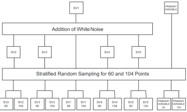
In this paper the influence of a secondary variable as a function of the correlation with the primary variable for collocated cokriging is examined. For this study five exhaustive data sets were generated in computer, from which samples with 60 and 104 data points were drawn using the stratified random sampling method.

These exhaustive data sets were generated departing from a pair of primary and secondary variables showing a good correlation. Then successive sets were generated by adding an amount of white noise in such a way

that the correlation gets poorer. Using these samples, it was possible to find out how primary and secondary

information is used to estimate an unsampled location according to the correlation level.

Key words: collocated cokriging, correlation coefficients, estimation weights, Markov Model Estimation,

multivariate geostatistics.

INTRODUCTION

The study of weights applied to variables in co-estimation must be an important issue when working with

cokriging techniques. Weights are assigned based on the spatial variance of the phenomenon under study. In this

sense, the further a sample is located from the point being estimated, the lower will be the weight assigned to it. It is already known that weights are constrained to different conditions in order to obtain a minimum estimation error-variance. These conditions depend on the cokriging technique applied. For example, in simple cokriging and collocated simple cokriging, there is no restriction to weights since in these cases global means are known. On the other hand, in ordinary cokriging it is necessary that primary and secondary weights sum up to one and zero, respectively, whereas in collocated ordinary cokri ging the sum of all weights must be one. These conditions, together with normal equations, form the cokriging systems whose resolution provides the weights for each sample.

Neither the knowledge about the behavior of weights under these restrictions nor the changes that

occur in this behavior when sample correlation coefficient varies are well comprehended yet. Conde (2000) studied ordinary cokriging applied to variables with different correlation coefficients. In the case of isotopic

sampling, average and variance values presented small variation as the correlation diminished. For partial

Correspondence to: Marcelo Monteiro da Rocha E-mail: mmrocha@usp.br

heterotopic sampling, variance values increased with the reduction of correlation, leading to the conclusion that, in such case, the method is not enough reliable.

As already mentioned, the weights that are assigned to secondary and primary variables in ordinary

collocated cokriging are constrained to some conditions, but it does not mean that they are sufficient to

guarantee consistent estimates. For instance, one problem is the enlargement of the estimated values range. Thus, the knowledge about which weight is assigned to each variable in different situations is necessary to control results in order to obtain better ones.

Thus, the aim of this paper is to investigate the influence of a secondary variable in the estimate of a primary variable by ordinary collocated cokriging. More specifically, it is intended to analyze the weights assigned to both variables in situations in which they present different correlation coefficients.

COKRIGING

Cokriging techniques constitute an attractive alternative and are commonly used when there is a variable of interest (primary variable) whose sampling is poor, and other variables (secondary variables) more densely sampled. These techniques work as follows: the estimates of a primary variable at unsampled locations are done considering not only primary data, but also secondary information.

According to Journel and Huijbregts (1978), the major contribution of cokriging to mining is the

possibility of co-estimating poorly sampled variables, but Olea (1991) and Myers (1982) mention that the best advantages are the reduction of error-variance estimation and the opportunity of estimating many attributes in the same domain.

According to Olea (1999), the absence of primary or secondary information in one or more points of

database does not constitute a problem since cokriging shows to be more efficient in this case. Instead,

Isaaks and Srivastava (1989) mention that cokriging does not show any advantage regarding kriging when both variables are sampled in all locations.

Several authors like Isaaks and Srivastava (1989) and Wackernagel (1998, 2003) also mention that

cokriging results are identical to the kriging ones when spatial correlation between primary and secondary variables is absent. In cases of isotopic sampling, cokriging is not worthwhile, and also when a secondary variable is available at the estimate location, the approximation of retaining only the collocated secondary data affects little prediction performance (Goovaerts 1998).

COLLOCATED COKRIGING

Among several cokriging techniques, collocated cokriging can be used in cases of heterotopic sampling.

More specifically, it can be applied when primary data are present in sparsely distributed points while

secondary data are located in all points of the grid being estimated.

In this case, the option for collocated cokriging is an attempt to avoid matrix instability that comes out from the application of ordinary cokriging. This problem is a direct consequence of a high auto-correlation between closer secondary data as opposed to lower auto-correlation and more distant primary data, resulting

in negative co-estimates (Xu et al. 1992, Wackernagel 2003). According to Xu et al. (1992), another reason

for choosing collocated cokriging is the need of eliminating redundant information since secondary data

According to Xu et al. (1992), for ordinary collocated cokriging the estimator is:

Z1 (xo)–m1 =

∑

2_[Z

2 (xo)–m2]

n1 * 1 α=1 * P S 1 S

∑

n P

i=1

S

∑

n P

i=1

∑

∑

n m

P S

i=1 j=1

where Z1 (xo) is the primary variable estimate; m1 and m2 are the average of primary and secondary variable populations, respectively Z1(xα) is the sampled primary variable; and Z2(xo) is the secondary variable

sampled at the same location where the primary variable will be estimated. The system from which primary and secondary weights (λα or λi and λ2 or λj, respectively) are obtained is:

where C11 (·) and C22 (·) are the spatial covariances of primary and secondary variables, respectively; C12 (·) is the cross-covariance between primary and secondary variables; and µ is the Lagrange multiplier.

Covariances C11 (h) and C22 (h) and cross-covariances C12 (h) = C21 (h) can be obtained by calculating and modeling, respectively, experimental variograms and cross-variograms under a valid corregionalization

linear model. However, according to Journel (1999) and Goovaerts (1997), depending on the number of

variables, this constitutes an unattractive procedure because variogram modeling becomes more complex since models cannot be built independently from each other.

A solution to this drawback, according to Xu et al. (1992), is to assume the Markov-type screening

hypothesis from which the influence of any primary data Z1 (x+h) on secondary collocated variable Z2 (x) is screened by the primary data Z1 (x). These authors also mention that the practical result of this hypothesis is the calculation of C12 (h) = C21 (h) from C11 (h) as follows:

C12 (h) = C11(h), 8h

C11(0)

C12(0)

ρ12 (h) = ρ12(0)ρ1(h), 8h

where C12 (0) is the spatial cross-covariance between primary and secondary variables at null distances, and

C11 (0) is the spatial covariance of primary variable at null distances. Equivalently, the cross-covariance can be written as (Xu et al. 1992):

where ρ1 (·) is the correlogram function of primary; variable and ρ12 (·) is the cross-correlogram function between primary and secondary variables.

Under the Markov model, the collocated co-kriging estimator can be written in its standardized form (Xu et al. 1992):

Thus, the primary variable was estimated by a collocated cokriging considering 60 or 104 points (Figure 3) with primary and secondary information. Besides collocated points present only information about the secondary variable.

For a better understanding, the procedures and resulting samples used in this paper are summarized in Figure 4.

Thus, for each sample composed of 60 and 104 collocated data points, we have estimated a regular grid such as the grid of exhaustive data sets (both PV and SVs). Since the exhaustive data sets present 3404 data points, the samples represent 1.76% and 3.06% of original populations. Unsampled data points were

estimated by collocated cokriging as defined by Xu et al. (1992).

σ1 σ1 σ2

Z1 *(xo)–m1 =

∑

n1

1 α=1

[Z1 (xα)–m1]

+ λ2 [Z2 (xo)–m2]

where σ1 and σ2 are stationary standard deviations associated with means m1 and m2 for variables Z1 and Z2, respectively. The collocated co-kriging equations can be, after Xu et al. (1992), written in its standardized form:

∑

ρ

2 ρ

12(0)ρ1 (xo–xα)= ρ1 (xo–xα) for α = 1, n1

n1

1 β=1

∑

ρ

2

= ρ12 (0)

n1

1 β=1

MATERIALS AND METHODS

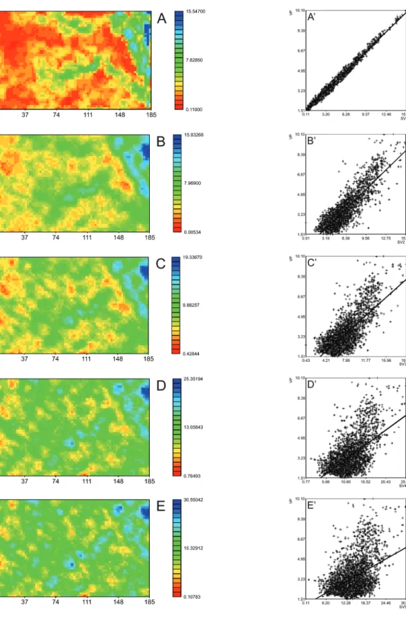
For this work a data set composed of both primary( Figure 1) and secondary (Figure 2) variables was

considered. We have departed from a secondary variable SV1 presenting high correlation coefficient with primary variable (PV) as shown in Figure 2A’. Since the idea of this paper is to test the influence of correlation

between PV and SV’s, we have generated secondary variables (SV2, SV3, SV4 and SV5) presenting lower

correlation coefficients by adding an increased percentage of white noise. From each complete data set of all these variables and of the primary one, stratified random samples with 60 and 104 points were drawn.

In order to perform the collocated coestimation, we used an isotropic variogram for the primary variable

to which an exponential model with sill equal to 5.27, a nugget effect of 0.001 and a range of 55.6 was fi tted.

RESULTS AND DISCUSSION

In this paper we want to examine the infl uence of the correlation coeffi cient in collocated cokriging.

Actually, we have to analyze the sum of primary variable weights and compare it to the secondary variable weights. This paper presents the results of a research project done by the authors and presented as a master

thesis by Watanabe (2008).

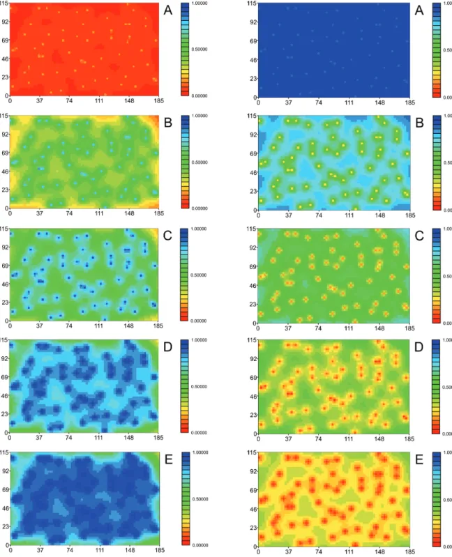
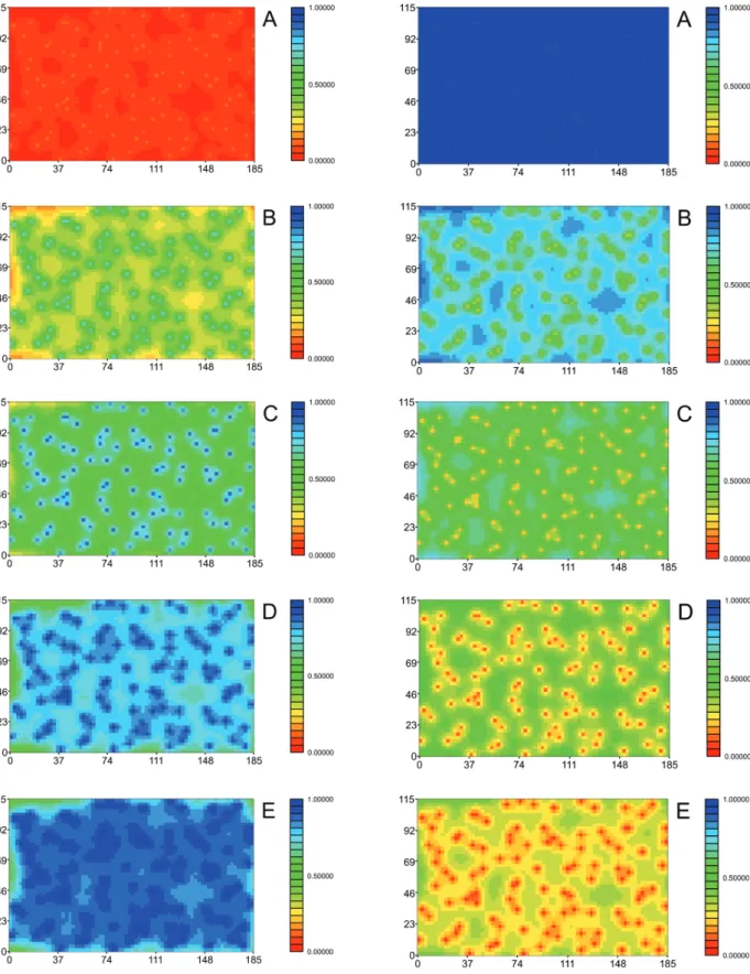
Figures 5 and 6 present results as image maps for the sum of PV and SV weights, respectively, for

samples with 60 and 104 allocated data points. Both fi gures show the same behavior for the sum of PV and SV weights. The higher the correlation, the higher is the infl uence of a secondary variable. On the other hand, when correlation goes down, the infl uence of primary variable goes up. This is the most interesting

result of this study, which shows clearly that, when the correlation is low or weak, the primary variable Figure 3: Location maps for 60 (left) and 104 (right) points obtained by stratifi ed random sampling (Watanabe 2008).

is retained as the more reliable information. Moreover, for cases of low correlation coefficients between

primary and secondary variables only locations around collocated data points are well co-estimated. In other words, when an unsampled location gets further from data points, the estimated value is poorly estimated since the secondary variable does not help in the co-estimation process.

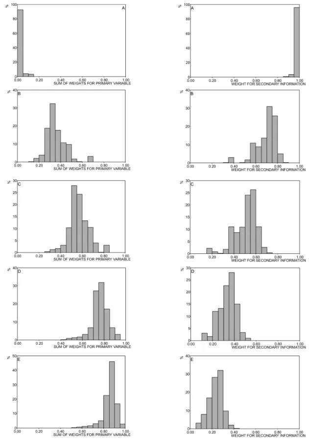
Histograms for the sum of PV and SV weights confirm the same behavior as described before (figures

7 and 8). Moreover, these histograms show the complementary character of both distributions for a same

correlation coefficient. For example, Figure 7A (on both sides) shows that almost all classes of the histogram

for the sum of PV weights are less than 0.20, whereas for SV weights almost all classes are greater than 0.80.

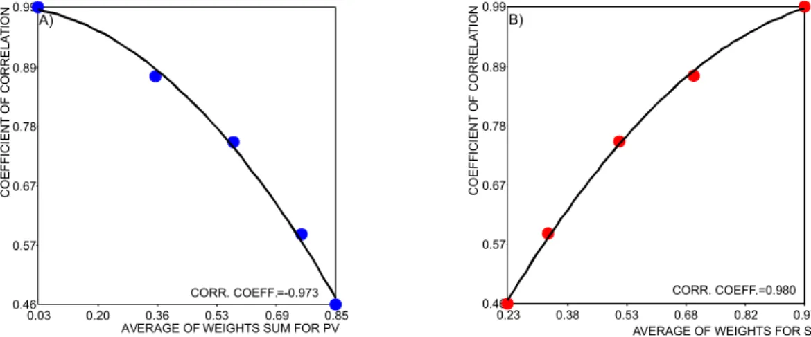
It is clear that there is a mutual relationship between the correlation coefficient and the sum of PV or

SV weights. In order to get this relationship we can compute for every correlation level the mean of sum

of PV weights and the mean of SV weights and display them in a graphic (figures 9 and 10). These figures summarize what we have seen regarding the sum of PV and SV weights. When correlation goes down, the mean of sum of PV weights goes up, whereas when the correlation coefficient increases, the mean of SV weights also increases according to a second degree polynomial function. Correlation coefficients between data points and a second degree function confirm the goodness of fit.

Figure 9: Relation between the correlation coefficient and the average sum of weights for primary variable (A) and secondary variable’s weight (B) considering 60 points (Watanabe 2008).

Figure 10: Relation between the correlation coefficient and the average sum of weights for primary variable (A) and secondary variable’s weight (B) considering 104 points (Watanabe 2008).

CONCLUSIONS

This paper showed how the correlation between primary and secondary variables influences the use of either primary or secondary information. When primary and secondary variables are well correlated, estimates are

done based on the secondary information. On the other hand, when the correlation is poor, then the primary information is used to estimate unsampled locations. Actually, when the correlation is poor, the ordinary kriging of the primary variable gives results as close as collocated cokriging ones.

Finally, when we have collocated data points, the sample size does not change significantly the

estimation results. 0.46 0.57 0.67 0.78 0.89 0.99

0.04 0.19 0.35 0.51 0.67 0.83 AVERAGE OF WEIGHTS SUM FOR PV

CORR. COEFF.=-0.957 A) C O E F F IC IE N T O F C O R R E L A T IO N 0.46 0.57 0.67 0.78 0.89 0.99

0.22 0.37 0.52 0.67 0.820 .97

AVERAGE OF WEIGHTS FOR SV CORR. COEFF.=0.971 B) C O E F F IC IE N T O F C O R R E L A T IO N

AVERAGE OF WEIGHTS SUM FOR PV CORR. COEFF.=-0.973 C O E F F IC IE N T O F C O R R E L A T IO N 0.46 0.57 0.67 0.78 0.89 0.99

0.03 0.20 0.36 0.53 0.69 0.85

A)

AVERAGE OF WEIGHTS FOR SV CORR. COEFF.=0.980 C O E F F IC IE N T O F C O R R E L A T IO N 0.46 0.57 0.67 0.78 0.89 0.99

0.23 0.38 0.53 0.68 0.82 0.97

ACKNOWLEDGMENTS

The authors want to thank Fundação de Amparo à Pesquisa do Estado de São Paulo (FAPESP), process

03/10367-7, for the financial support.

RESUMO

Neste artigo examina-se a influência da variável secundária como função da correlação com a variável primária na

cokrigagem colocalizada. Para este estudo cinco bases de dados completas foram geradas no computador a partir das quais amostras com 60 e 104 pontos de dados foram retirados através do método de amostragem aleatória

estratificada. Estas bases de dados completas foram geradas partindo-se de um par de variáveis, primária e secundária,

que apresentam boa correlação. Então sucessivos conjuntos foram gerados adicionando-se uma quantidade de ruído branco de modo que a correlação se tornasse menor. Utilizando-se estas amostras foi possível encontrar o quanto as informações primária e secundária são utilizadas na estimativa de um ponto não amostrado conforme o nível de correlação.

Palavras-chave: cokrigagem colocalizada, coeficientes de correlação, pesos de estimativa, Modelo de Markov,

geoestatística multivariada

REFERENCES

CONDE RP. 2000. Geoestatística Aplicada a Avaliação de Reservas e Controle de Lavra na Mina de Cana Brava (GO).

Tese de Doutoramento apresentada no Instituto de Geociências – USP, 162 p.

GOOVAERTS P.1997. Geostatistics for natural resources evaluation. Oxford University Press, New York, 483 p.

GOOVAERTS P.1998. Ordinary Cokriging Revisited. Math Geol 30(1): 21–42.

ISAAKS EH AND SRIVASTAVA RM.1989. An introduction to applied geostatistics. Oxford University Press, New York, 561 p.

JOURNEL AG.1999. Markov Models for Cross-Covariances. Math Geol 31(8): 955-964.

JOURNEL AG AND HUIJBREGTS CJ.1978. Mining geostatistics. Academic Press, 600 p.

MYERS DE. 1982.Matrix formulation of Co-Kriging. Math. Geol 14: 249 – 257.

OLEA R.1991. Geostatistical Glossary and Multilingual Dictionary. 1st ed., Oxford University Press, Oxford, 175 p. OLEA R.1999. Geostatistics for Engineers and Earth Scientists. 1st ed., Kluwer Academic Publishers, Massachusetts, 303 p.

WACKERNAGEL H.1998. Multivariate Geostatistics. 2nd ed., Springer-Verlag, Berlin, 291 p.

WACKERNAGEL H.2003. Multivariate Geostatistics. 3rd ed., Springer-Verlag, Berlin, 387 p.

WATANABE J.2008. Métodos geoestatísticos de co-estimativas: Estudo do efeito da correlação entre variáveis na precisão dos

resultados. Dissertação de Mestrado, Instituto de Geociências – USP, 79 p. (Unpublished).

XU W, TRAN TT, SRIVASTAVA RM AND JOURNEL AG. 1992. Integrating Seismic Data in Reservoir Modelling:

The Collocated Cokriging Alternative. In: Annual Technical Conference of the SPE, 67, Washington, Proceedings, paper SPE