Evaluation of sugarcane genotypes and production environments in
Paraná by GGE biplot and AMMI analysis
Pedro Henrique Costa de Mattos1*, Ricardo Augusto de Oliveira1, João Carlos Bespalhok Filho1, Edelclaiton Daros1 and Mario Alvaro Aloiso Veríssimo1
Received 29 November 2012 Accepted 18 February 2013
Abstract– The purpose of this study was to evaluate sugarcane genotypes for the trait tons of sugar per hectare (TSH), stratifying five production environments in the state of Paraná. The performance of 20 genotypes and 2 standard cultivars was analyzed in three consecutive growing seasons by the statistical methods AMMI and GGE Biplot. The GGE Biplot grouped the locations into two mega-environments and indicated the best-performing genotypes for each one, facilitating the selection of superior genotypes. Another advantage of GGEBiplot is the definition of an ideal genotype (G) and environment (E), serving as reference for the evaluation of genotypes and choice of environments with greater GE interaction. Both models indicated RB006970, RB855156 and RB855453 as the genotypes with highest TSH and São Pedro do Ivai as the environment with the greatest GE interaction. Both approaches explained a high percentage of the sum of squares, with a slight advantage of AMMI over GGE Biplot analysis.
Key words: Saccharum spp., adaptability, stability, environment stratification.
1 Universidade Federal do Paraná (UFPR), SCA, DFF, Rua dos Funcionários, 1540, 80.035-050, Juvevê, Curitiba, PR, Brazil. *E-mail: [email protected]
INTRODUCTION
The development of sugarcane and other crops is af-fected by effects of the environment (E), genotype (G) and
their interaction (GE), of which the latter causes significant
variations in cultivar performance between different loca-tions (Mohammadi et al. 2007).
The evaluation of genotypes, aside from the stratifica -tion of produc-tion environments, is fundamental for the study of relations between genotypes and environments (GE), especially to identify similar response patterns of genotypes in the environments of the experimental network (Cruz et al. 2001).
One of the most recent evaluation methods is the AMMI (Additive Main Effects and Multiplicative Interaction) analysis. In this model, statistical techniques such as analysis of variance and principal component analysis, respectively, are combined to adjust the main effects and GE interaction effects (Duarte and Vencovsky 1999).
Yan et al. (2000) proposed the GGE Biplot method and pointed out that although the yield data are the combined
effect of genotype (G), environment (E) and the interaction of both (GE), only G and GE are relevant and should be considered simultaneously in the evaluation of genotypes. Furthermore, the biplot technique is also used to approach and evidence the G and GE effect in a multi-environmental trial, which coined the term “GGE Biplot”.
Recently, several methods were used simultaneously to evaluate genotypes and production environments of different crops (Silva and Duarte 2006, Cargnelluti Filho et al. 2007, Melo et al. 2007, Silva Filho et al. 2008, Pereira et al. 2009, Guerra et al. 2010, Nunes et al. 2011, Gouvêa et al. 2011). However, the AMMI has seldom been used together with the GGE Biplot in studies on sugarcane. Other crops, for example, wheat (Kaya et al. 2006, Yan et al. 2007), soybean (Asfaw et al. 2009), sorghum (Rao et al. 2011), and carrot (Silva et al. 2012) were evaluated.
The objective of this study was to evaluate 22 sugar-cane genotypes in 5 production environments, based on the adaptability and stability of genotypes using 2 statistical methods, GGEBiplot and AMMI.
Crop Breeding and Applied Biotechnology 13: 83-90, 2013 Brazilian Society of Plant Breeding. Printed in Brazil
MATERIALS AND METHODS
We evaluated 20 sugarcane genotypes, plus 2 cultivars as controls: RB855156 and RB855453 in the growing seasons of 2009/10, 2010/11 and 2011/12.
The tests were conducted in five environments: Astorga
(23°05’S, 51°36’W, 634 m asl), Bandeirantes (lat 23º 06’S, long 50° 22’ W, and alt 492 m asl), Colorado (lat 22° 50’ S, long 51° 54’ W, and alt 400 m asl), Goioerê (lat 24° 10’ S, long 53º 01’ W, and alt 550 m asl) and São Pedro do Ivai (lat 23° 52’ S, long 51° 41’ W, and alt 40 m asl), in the state of Paraná. The climate in all environments was Cfa, according to Köppen.
The experiments were arranged in a randomized complete block design with three replications in plots of four 8m-rows spaced 1.40 m apart. In March 2009, 18 buds were planted per meter. The harvest of each growing seasons occurred in April 2010, 2011 and 2012. At harvest, three samples of 15 stalks without tips per plot were collected without burning the sugarcane from the two central rows, while in front and at the end of the plot, 1 meter was not evaluated (border). The samples were used to estimate the average weight per stalk (M1C) and the trait pol % cane (PC). The number of stalks per plot was also counted, to determine the number of stalks per meter (NSM). These values were used to
de-fine the traits of tons of stalks per hectare (TSH) and tons
of sugar per hectare (TSH), by the following expressions:
TSH = NCM x MIC x 7.142, where the fixed value 7.142
indicates the area estimated for planting, according to the spacing and TSH = (TSH x PC)/100.
Based on the TSH data, analyses of variance were conducted for each production environment and for plant
cane, first ratoon and second ratoon. Once the differences
between the treatments were detected, combined analysis of variance was performed (Ramalho et al. 2000), providing complementary information to the analysis.
After detecting the GE interaction (P test significant) by
combined analysis of variance, the phenotypic adaptability and stability was analyzed by the GGEBiplot (Yan et al. 2000) and AMMI methods (Zobel et al. 1988).
The first evaluation was performed using the GGEBiplot,
based on the following model: yij - yj = y1εi1pj1 + y2εi2pj2, where: yij represents the average yield of the i-th population in the j-th environment; yiis the overall mean of population j in environment j; y1εi1pj1 is the first principal component (PCI1); y2εi2pj2 is the second major component (PCI2); y1, y2 are the eigenvalues associated to PCI1 and PCI2,
respectively; ε1 and ε2 are the scores of the first and sec -ond main component, respectively, of the i-th population;
pj1 and pj2 are the scores of the first and second principal component, respectively, for the j-th environment; and εij is the error associated with the model of the i-th population and j-th environment (Yan and Kang 2003).
The second analysis applied AMMI, based on the model described by Duarte and Vencovsky (1999):
yij = μ + gi + ai +
∑
nk=1 λkγikαjk + ρij + εij;
where: yij is the mean response of genotype i (i = 1, 2, ..., G genotypes) in environment j (j = 1, 2, ..., A environ-ments), μ is the overall mean of the tests; gi is the fixed effect of genotype i (i = 1, 2,... g); and αj is the random effect of environment j (j = 1, 2, ... a). The GE interaction
is influenced by the factors: λk, which is the singular value for the k-th principal component of interaction (PCI), (k = 1, 2, ... p, where p is the maximum number of estimable principal components); yjk is the singular value of the j-th environment in the k-th PCI; αik is the singular value of the i-th genotype in the k-th PCI; k are nonzero characteristic roots, k = [1, 2, .. . min (g-1 e-1)]. Item ρ is the residue of the GE interaction or AMMI residue (noise in the data) and ε is the average experimental error, assumed as independent.
RESULTS AND DISCUSSION
The combined analysis showed that the yield of sugarcane
genotypes was significantly influenced by the environment
(E), which explained 70.5% of the total phenotypic variation while the genotypic traits (G) and the interaction between genotype and environment (GE) explained 10.43 and 10%, respectively, of the total variation (Table 1). Gauch and Zobel (1996) reported that in multi-environment trials, the environment (E) normally explains up to 80% of the varia-tion while genotype (G) and the genotype - environment (GE) interaction both usually represent around 10 - 15% of each variation.
The analysis of variance also showed that the effects of sources of variation, genotype, environment, and GE
inter-action were significant for the variable analyzed (Table 1).
This result indicated that the genotypes were characterized as environmentally-induced changes.
For the percentage of explanation of the interaction axes
of AMMI and GGE Biplot, it was observed that the first
For the methodologies that use principal component
analysis, the first interaction axes contain a greater standard
percentage, with a decrease in the subsequent axes. Thus, as the number of selected axes is increased, the noise percent-age increases, reducing the predictive power of the analysis
(Oliveira et al. 2003). Based on this definition and the high
accumulated value of explanation of percentages of the
sum of the squares on the two first axes of interaction by
both approaches (Table 1), the adaptability and stability of sugarcane genotypes can be graphically interpreted,
consid-ering only biplots with the first two axes of GE interaction.
The values of TSH were highest for the genotypes RB006991 (G19), RB006970 (G10), RB005916 (G1), RB005935 (G4) and RB855156 (G21), respectively, in Astorga, Bandeirantes, Colorado, Goioerê, and São Pedro do Ivai (Table 7).
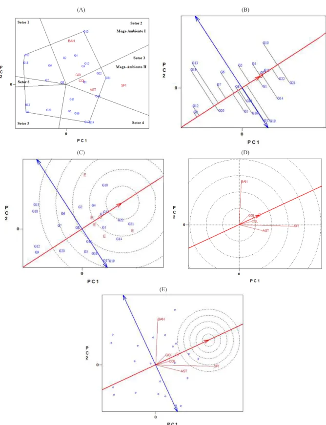
Figure 1A of the GGE Biplot analysis is important to study the possible existence of mega-environments within a growing region (Yan and Rajcan 2002). A polygon was drawn connecting the genotypes that are further away from the biplot origin, (RB855156 (G21), RB006970 (G10), RB006973 (G13), RB006988 (G18), RB005991 (G9), RB006991 (G19)) (Figure 1A). These genotypes have the largest vectors in their respective directions; the vector length and direction represent the extent of the response of the genotypes to the tested environments. All other genotypes are contained within the polygon and have smaller vectors, i.e., they are less responsive in relation to the interaction with the environments within that sector. The vectors originating from the center of the biplot (0; 0), perpendicular to the sides of the polygon, divided the graph into six sectors (Figure 1).
The polygon of the GGE biplot (Figure 1A) grouped the test locations in mega-environments. Mega-environments are those sectors which comprise one or more environments. In this case, there were two mega-environments: I - Astorga, Colorado and São Pedro do Ivai and II - Bandeirantes and Goioerê.
In Figure 1A, the genotype of the vertex of the polygon, contained in a mega-environment, had the highest yield in at least one environment and was one of the best-performing genotypes in the other environments (Yan and Rajcan 2002). Thus, genotype RB855156 (G21) was the best in São Pedro do Ivai and performed well in Colorado and Astorga and genotype RB006970 (G10) obtained highest yields in Bandeirante and was among the best in Goioerê (Figure 1A and Table 2).
The genotype yield and stability were evaluated from the average environment coordination (AEC) (Yan and Rajcan 2002). The greater the projection of the genotype on the axis of the AEC ordinate, the greater the instabil-ity of the genotype, representing a greater interaction with the environments. In this sense, the genotypes G22 (RB85545), G15 (RB006976), G3 (RB005924), G4
(RB005935), and G1 (RB005916) were identified as the
most stable. Although the yield variation of genotypes G21 (RB855156) and G10 (RB006970) was great, they were always among the best genotypes in all tested envi-ronments (Figure 1B and Table 2). Based on the average
TSH yield in the three seasons and at the five locations,
the genotypes with above-average yields were ranked in decreasing order: G21 (RB855156), G10 (RB006970), G22, G15, G3, G14, G4, G1, G2, G19, and G17.
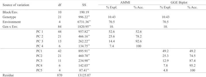
Table 1.Combined analysis of variance for tons of sugar per hectare (TSH) and proportion of the sum of squares of genotype - environment interaction for each axis of the main components of the GGE Biplot and AMMI analyses for 22 sugarcane genotypes in five environments in the State of Paraná.
Source of variation df SS AMMI GGE Biplot
% Expl. % Acc. % Expl. % Acc.
Block/Env. 10 190.19
Genotype 21 996.22** 10.43 10.43
Environment 4 6731.36** 70.5 70.5
Gen x Env. 84 1820.95** 10. 10.
PC 1 44 957.82** 52.6 52.6 PC 2 21 466.16** 25.6 78.2 PC 3 13 262.22** 14.4 92.6 PC 4 6 134.75** 7.4 100
PC1 42 895.91** 49.2 49.2
PC2 21 460.70** 25.3 74.5
PC3 11 234.90** 12.9 87.4
PC4 6 142.03** 7.8 95.2
PC5 4 87.41** 4.8 100
Residue 870 13125.07
An ideal genotype should have an invariably high average yield in all environments concerned. This ideal genotype is
graphically defined by the longest vector in PC1 and without
projections in PC2, represented by the arrow in the center of the concentric circles (Figure 1C). Although this genotype is but an estimate, it is used as a reference for the evaluation of genotypes. The standard cultivars RB855156 (G21) and RB855453 (G22), and genotype RB006970 (G10), RB006976 (G15), RB005924 (G3), RB005935 (G4) and RB005916 (G1) were contained in the second concentric circle (Figure 1C); these genotypes are closest to the ideal and can be considered desirable in terms of yield and stability of the trait TSH.
Figure 1D shows the relationship between yield and sta-bility from the vectorial standpoint of the environments, and they are connected by vectors with the origin of the biplot. In environments with small vectors, the yield stability is high. The difference between the average yield of genotypes was lowest in Colorado and Goioerê (Figure 1D and Table 2), i.e., they contributed less to the GE interaction.
For environments that contributed most to the GE in-teraction, the environments Bandeirantes and São Pedro do Ivai were the most unstable, in other words, the interaction between genotypes and environments was greater (Figure
1D). In this figure, the values of the cosines of the angles
between the vectors of each environment corresponded to
the correlation coefficient between them. Most environments
are positively correlated, because the cosine of the angle between them is positive. The only exception was the correla-tion between Astorga and Bandeirantes, which is negative, i.e., the angle between their vectors is > 90 °. Positive and negative correlations between test environments were also detected by Kaya et al. (2006), who used the GGE biplot approach to assess wheat and its production environments.
An ideal environment should have a high PC1 score (greatest power of genotype discrimination in terms of main genotype effects) and zero score for PC2 (greatest repre-sentativeness of all other environments). In Figure 1E, this environment is represented on the axis of abscissa AEC by an arrow in the center of the concentric circles. Similarly to the ideal genotype, the ideal environment is only an estimate and serves as a reference for site selection for multi-environment trials. The most desirable is the one closest in the graph of the ideal environment (Yan and Rajcan 2002).
The environment São Pedro do Ivai contained in the
fifth concentric circle is the location with greatest ability to
discriminate genotypes, favoring the selection of superior
Table 2. Average production of tons of sugar per hectare (TSH) of the 22 sugarcane genotypes, in each of five tested environments and overall average
Label Genotype Astorga Bandeirantes Colorado Goioerê São Pedro do Ivaí Mean
G1 RB005916 11.67 14.83 12.19 11.82 18.13 13.73
G2 RB005918 10.25 16.66 10.06 11.84 16.71 13.11
G3 RB005924 11.45 16.00 9.82 12.89 18.32 13.70
G4 RB005935 9.21 15.87 10.54 15.73 17.77 13.83
G5 RB005968 9.01 12.70 7.65 10.93 18.70 11.80
G6 RB005971 12.32 16.20 9.08 12.42 14.19 12.85
G7 RB005982 9.51 14.80 8.54 12.14 15.27 12.06
G8 RB005987 8.68 14.49 9.20 12.30 17.30 12.40
G9 RB005991 8.35 12.14 7.38 12.20 13.82 10.78
G10 RB006970 11.86 18.96 9.47 12.32 18.46 14.22
G11 RB006971 12.30 13.83 8.90 11.50 17.08 12.73
G12 RB006972 9.60 12.79 9.79 11.57 12.71 11.30
G13 RB006973 8.62 16.74 8.23 11.53 13.29 11.69
G14 RB006974 12.85 13.57 9.10 14.53 19.38 13.89
G15 RB006976 10.51 16.22 9.19 12.61 19.27 13.56
G16 RB006981 11.39 12.47 9.71 11.92 17.82 12.67
G17 RB006984 12.96 12.05 9.76 11.77 18.38 12.99
G18 RB006988 10.98 16.14 8.98 12.48 11.82 12.08
G19 RB006991 13.74 12.23 9.79 11.24 18.70 13.14
G20 RB006992 11.12 12.38 10.56 12.51 14.28 12.18
G21 RB855156 12.73 14.94 10.48 14.44 20.29 14.58
G22 RB855453 12.10 15.44 11.30 12.97 19.54 14.27
Mean 10.97 14.61 9.53 12.44 16.87 12.889
(A) (B)
(C) (D)
(E)
Figure 1.GGE Biplot methodology, with the first two principal axes of the interaction (PC1 and PC2) for the average yield per ton of sugar per hectare
genotypes (Fig. 1E). In the same graph, Bandeirantes rep-resented a high yield potential, but no capacity of genotype discrimination, since the standard deviation between the mean TSH of the genotypes was lower than of São Pedro do Ivai (Table 6).
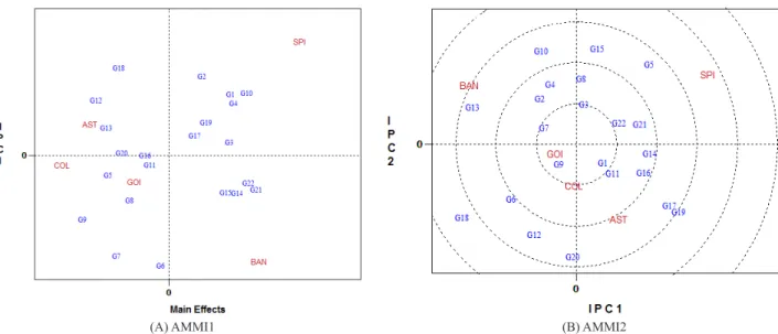
According to AMMI analysis, seven genotypes (RB006970 (G10), RB005916 (G1), RB005924 (G3), RB005935 (G4), RB006974 (G14), RB006976 (G15), and RB006961 (G19)), had an average yield similar to the con-trols (Figure 2A and Table 2), but only genotype RB005916 (G1) had above-average yield and low instability (Figure 2A, B). The stability of genotype RB005991 (G9) was high, compared with the standards, for being close to the origin of AMMI2, but its average yield was much lower than that of the other genotypes (Figure 1B and Table 2). In general, the most stable genotypes were RB005987 (G8), RB005916 (G1), RB855453 (G22), RB855156 (G21), RB006971 (G11), RB005935 (G4), and RB005982 (G7), because the GE interaction scores were lowest and positions closest to the center of the AMMI2biplot. In this same biplot, the most unstable genotypes were RB006970 (G10), RB006961 (G19) and RB006992 (G20), all distant from the center of AMMI2 biplot (Figure 1B).
Genotype RB006970 (G10) was one of the most
produc-tive and specifically adaptable to less restricproduc-tive environ -ments. The yield of this genotype was higher in environments with more clayey soils (Bandeirantes and São Pedro do Ivai), and reduced in sandy- soil environments (Colorado, Goioerê and Astorga) (Table 2). For genotype RB005916
(G1), high stability but low yield was found (Figure 2A and B and Table 2).
The environments Bandeirantes and São Pedro do Ivai contributed most to the GE interaction, that is, the instabil-ity was greatest, since the scores were the highest on the axes of interaction (Figure 2B). In turn, the more stable environments Astorga, Colorado and Goioerê had lower PCI1 scores (Figure 2B). Guerra et al. (2009) reported that environmental stability indicates the reliability of genotype ranking in a given test environment, in relation to the average
ranking of the tested environments. Based on this definition,
the greater stability of the locations Colorado, Goioerê and Astorga than of Bandeirantes and São Pedro do Ivai suggests
that the genotype classification of the former group should
have lower standard deviation of genotype performances
than the classification in other production environments.
Genotypes and environments with the same sign in the AMMI2 biplot (Figure 2B) must interact positively and if the signs are opposite, negatively (Duarte and Venkovsky 1999). Guerra et al. (2009) and Verissimo et al. (2012)
identified genotypes and environments with same-sign PCI scores, with positive specific interactions for sugarcane. The classification of genotypes and environments established by
Oliveira et al. (2003) and Silva et al. (2012) for soybean and carrot, respectively, was the same.
The environments Goioerê and Colorado lie very close to each other (Figure 2B) within the same quadrant and with the same sign, indicating similar genotype yields. The
(A) AMMI1 (B) AMMI2
Figure 2. Biplot AMMI1 (A) with the first principal axis of interaction (PCI1) x average yield of tons of sugar per hectare (TSH), and AMMI2 (B),
proximity of genotype RB005991 (G9) to environments
Goioerê and Colorado indicates a specific genotype adapt -ability to these environments.
The results of production environments with low GE interaction, as in Colorado and Goioerê, can be extrapolated to other environments. These can be used, for example, in the early stages of a sugarcane breeding program, using a large number of genotypes (seedlings) planted without replications and at only one location.
Conversely, highly instable production environments, i.e., with high GE interaction, as for example São Pedro do
Ivaí and Bandeirantes, should be used in genotype competi-tion trials, for facilitating the seleccompeti-tion of superior plants.
CONCLUSIONS
The stability and adaptability of GGE biplot and AMMI indicated the same genotypes RB006970, RB855156 and RB855453 as the most productive in tons of sugar per hectare (TSH) and also indicated São Pedro do Ivai as the environment with the greatest effect of GE interaction. The percentage of explanation of the sum of squares was high by both methods, with a small advantage of the AMMI over the GGE Biplot analysis.
Avaliação de genótipos de cana-de-açúcar e ambientes de produção no Paraná
via GGE Biplot e AMMI
Resumo– O objetivo deste trabalho foi avaliar genótipos de cana-de-açúcar, considerando toneladas de pol por hectare (TPH),
estratificando cinco ambientes de produção no Paraná. Foram analisados 20 genótipos e dois padrões, em três safras consecutivas. Os métodos estatísticos utilizados foram AMMI e GGE Biplot. O GGE Biplot agrupou os locais em dois mega-ambientes e apresen-tou quais genótipos estiveram entre os melhores para cada mega-ambiente, facilitando a seleção dos genótipos superiores. Outra vantagem do GGE Biplot foi a representação do genótipo e do ambiente ideal, que serviram de referência para a avaliação dos genótipos e para escolha de ambientes com maior interação GxE. Ambos os modelos, mostraram que os genótipos mais produtivos em TPH, foram: RB006970, RB855156 e RB855453 e que o ambiente São Pedro do Ivaí apresentou maior interação GxE. Ambas metodologias apresentaram elevada porcentagem de explicação das soma dos quadrados, tendo a metodologia AMMI uma pequena vantagem sobre o GGE Biplot.
Palavras-chave:Saccharum spp., adaptabilidade, estabilidade, estratificação ambiental.
REFERENCES
Asfaw A, Alemayehu F, Gurum F and Atnaf M (2009) AMMI and GGE Biplot analysis for matching varieties onto soybean production environments in Ethiopia. Scientific Research and Essay 4: 1322-1330.
Cargnelluti Filho A, Perecin D, Melheiros EB and Guadagnin JP (2007) Comparação de métodos de adaptabilidade e estabilidade relacionados a produtividade de grãos de cultivares de milho. Bragantia 66: 571-578.
Chavanne ER, Ostengo S, García MB and Cuenya MI (2007) Evaluación del comportamiento productivo de cultivares de caña de azúcar (Saccharum spp.) a través de diferentes ambientes en Tucumán, aplicando la técnica estadística “GGE biplot”. Revista industrial y
agrícola de Tucumán 84: 19-24.
Cruz CD and Regazzi AJ (2001) Modelos Biométricos aplicados ao melhoramento genético. Editora UFV, Viçosa, 390p.
Duarte JB and Venkovsky R (1999) Interação genótipos x ambientes:
uma introdução à análise “AMMI”. Editora FUNPEC, Ribeirão Preto, 60p.
Gauch HG and Zobel RW (1996) Optimal replication in selection experiments. Crop Science36: 838-843.
Gouvêa LRL, Silva GAP, Scaloppi Junior EJ and Gonçalves PS (2011) Different methods to assess yield temporal stability in rubber.
Pesquisa Agropecuária Brasileira 5: 491-498.
Guerra EP, Oliveira RA, Daros E, Zambon JLC, Ido OT and Bespalhok Filho JC (2009) Stability and adaptability of early-maturing sugarcane clones by AMMI analysis. Crop Breeding and Applied
Biotechnology 9: 260-267.
Kaya Y, Akçura M and Taner S (2006) GGE biplot analysis of multi-environment yield in bread wheat. Turkish Journal of Agriculture
and Forestry 30: 325-337.
Melo LC, Melo PGS, Faria LC, Dias JLC, Del Peloso MJ, Rava CA and Costa JGC (2007) Interação com ambientes e estabilidade de genótipos de feijoeiro-comum na Região Centro-Sul do Brasil.
Pesquisa Agropecuária Brasileira 3: 715-723.
Mohammadi R, Haghparast R, Aghaee M, Rostaee M and Pourdad SS
(2007) Biplot analysis of multi-environment trials for identification
of winter wheat megaenvironments in Iran. World Journal of
Agricultural Sciences 3: 475-480.
Nunes GHS, Andrade Neto RC, Costa Filho JH and Melo SB (2011)
Influência de variáveis ambientais sobre a interação genótipos
x ambientes em meloeiro. Revista Brasileira de Fruticultura 33:
Oliveira BA, Duarte JB and Pinheiro JB (2003) Emprego da análise AMMI na avaliação da estabilidade produtiva em soja. Pesquisa Agropecuária Brasileira38: 357-364.
Pereira HS, Melo IC, Del Peloso MJ, Faria LC, Costa JGC, Cabrera Dias JL, Rava CA and Wendland A (2009) Comparação de métodos de análise de adaptabilidade e estabilidade fenotípica em feijoeiro-comum. Pesquisa Agropecuária Brasileira 44: 374-383.
Ramalho MAP, Ferreira DF and Oliveira AC (2000) Experimentação em genética e melhoramento de plantas. Editora UFLA, Lavras, 326p.
Rao PS, Reddy PS, Rathore A, Reddy BV and Panwar S (2011) Application GGE biplot and AMMI model to evaluate sweet sorghum hybrids for genotype x environment interaction and seasonal adaptation. Indian
Journal of Agricultural Sciences 81: 438-444.
Silva GO, Carvalho ADF, Vieira JV and Benin G (2012) Verificação da
adaptabilidade e estabilidade de populações de cenoura pelos métodos AMMI, GGE biplot e REML/BLU. Bragantia 9: 269-274.
Silva WCJ and Duarte JB (2006) Métodos Estatísticos para estudo de adaptabilidade e estabilidade fenotípica em soja. Pesquisa
Agropecuária Brasileira 41: 23-30.
Silva Filho JL, Morello CL, Farias FJC, Lamas FM, Pedrosa MB and Ribeiro FL (2008) Comparação de métodos para avaliar a adaptabilidade e estabilidade produtiva em algodoeiro. Pesquisa
Agropecuária Brasileira 43: 349-355.
Verissimo MAA, Silva DAS, Aires RF, Daros E and Panziera W (2012) Adaptabilidade e estabilidade de genótipos precoces de cana-de-açúcar no Rio Grande do Sul. Pesquisa Agropecuária Brasileira
47: 561-568.
Yan W, Hunt LA, Sheng QL and Szlavnics Z (2000) Cultivar evaluation and mega-environment investigation based on the GGE Biplot. Crop
Science 40: 597-605.
Yan W and Kang MS (2003) GGE Biplot analysis: a graphical tool for
breeders, geneticists, and agronomists. CRC Press, Boca Raton, 288p.
Yan W and Rajcan I (2002) Biplot evaluation of test sites and trait relations of soybean in Ontario. Crop Science 42: 11-20.
Yan W, Kang MS, Ma B, Woods S and Cornelius PL (2007) GGE Biplots vs. AMMI analysis of genotype-by-environment data. Crop Science
47: 643-655.