Budgetary decomposition and yield spreads

António Afonso, João Tovar Jalles

Budgetary Decomposition and Yield

Spreads

W

P

Budgetary Decomposition and Yield

Spreads

*

António Afonso

João Tovar Jalles

December 2015

Abstract

With a panel VAR of 10 Euro area countries we study the budgetary determinants of government bond yield spreads vis-à-vis Germany between 1999Q1 and 2012Q4. We find that rising bid ask, VIX and debt differentials increase yield spreads; and improvements in the budget balance, higher growth prospects and depreciation lower the spreads. Moreover, rises in public wages or in social expenditure increase spreads, while increases in direct and indirect taxes lower the yield spreads. In the post-2007Q3 crisis period, rising expenditure components (except subsidies) increased spreads.

JEL: C23, E62, G01, H62,

Keywords: fiscal components, bond yields, Great Recession, PVAR, impulse responses.

*

The opinions expressed herein are those of the authors and do not reflect those of their employers.

$

ISEG/UL - University of Lisbon, Department of Economics; UECE – Research Unit on Complexity and Economics. UECE is supported by FCT (Fundação para a Ciência e a Tecnologia, Portugal), email: [email protected].

2 1. Introduction

Government bond yield spreads are a collective expression of differences in levels of development, risk, expected return and other essential features of countries or regions whose bond yields we would like to compare. Since the onset of the 2008-2009 global financial crisis, the international risk aversion has increased and market participants have priced sovereign bonds higher relative to German safe haven, and markets have become more sensitive to fiscal imbalances. In addition to increasing the costs of borrowing, a rise in spreads signals that investors have less motivation to lend funds, constraining a country’s access to international capital markets.

Therefore, fiscal policy could be among the most important determinants of yields and spreads of government bonds. Also important is the capacity of the fiscal policy makers to increase tax revenue and take on credit to finance public expenditure while minimizing the growth-hindering costs. It is expected that a better and more trustworthy fiscal policy will reduce risks, tend to produce a better organization of public debt instruments and in general underpinning economic growth.

We study the determinants of observed yield spreads differentials against Germany using a panel of ten Euro area countries for the period of 1999Q1 to 2012Q4. First, this is a relevant country sample to study sovereign yield differentials because in the Economic and Monetary Union (EMU) there are different sovereign issuers, without the noise arising from different currencies or bond conventions. Second, even though the start of the EMU led to a sharp decline in 10-year government bond yield spreads against the German benchmark, these bonds are not perfect substitutes. Indeed, with the global financial crisis, bond yield differentials witnessed large increases for several periphery countries. Third, we evaluate the budgetary determinants of yield spreads differentials, looking at both revenue and expenditure components. Fourth, we use higher frequency data, since quarterly fiscal data, for this set of euro area countries has not been widely employed, and quarterly indicators can reveal essential information about the sustainability of fiscal policy.

2. Literature

There is a consensus in the literature as to the main factors affecting yield spreads. First,

credit risk, since differences in government bond yields related to fiscal vulnerabilities and

default risks. Countries’ debt sustainability is priced by markets and despite the Stability Pact, EMU countries are perceived as having different credit risk. Studies have shown that the

deterioration of a country’s fiscal position can explain interest rate differentials between the EMU countries (Ardagna et al, 2007; Manganelli, 2009; Bernoth, 2012).

Second, liquidity risk, and in a liquid market there is a large-scale transactions impinge less on prices (Barrios 2009), this allows differences between government bonds yields. Nevertheless, Codogno et al. (2003) and Favero et al (2010) find that liquidity has small explaining power whereas Ejsing et al. (2011) shows that the liquidity of sovereign bond markets is important in explaining spread behavior.

Third, risk aversion, given that in periods of higher uncertainty investors tend to be more risk averse and to invest in less risky securities. In the EMU, German bonds are perceived as the “safe haven” because of their credit quality and liquidity. Several studies have shown that sovereign yield differentials can be explained by international factors and investors’ risk aversion (Manganelli, 2009, Favero et al, 2010, Longstaff, 2011).

3. Methodology and data

We use a Panel Vector Autoregression (PVAR) to analyze the short-run transition of spreads to shocks to “fundamental” and budgetary variables. Take a first-order VAR model as: t i i t i t i LY Y_, ₀ ( ) _,  _,, (1)

where Yi,t is a vector of endogenous variables, 0 is a vector of constants, (L)is a matrix

polynomial in the lag operator, _i is a matrix of country-specific fixed effects, and _i,t is a vector of error terms. The correlation between fixed effects and regressors due to lags of the dependent variables implies that the mean-differencing procedure creates biased coefficients (Holtz-Eaking et al., 1988). This drawback is solved using the “Helmert procedure”1 and estimating a system by GMM using the lags of the regressors as instruments. In our model, the number of regressors is equal to the number of instruments. As far as impulse-response functions are concerned, given that the variance-covariance matrix of the error terms may not be diagonal, we follow the Choleski decomposition.

We use quarterly data on 10 EMU countries covering a maximum time span of 1999Q1 to 2012Q4.2 The main variable of interest is the 10-year government bond yield spread versus Germany, . Figure 1 displays its evolution. After 1999 spreads in have

1 _{This is a forward mean-differencing approach that removes only the mean of all future observations available}

for each country-year.

2

4

converged to very low levels despite the fact that macroeconomic fundamentals where different between countries, suggesting these were not properly priced by markets. During the global financial crisis almost all countries saw a large increase in their spreads.

[Figure 1]

In addition to the yield spreads, the vector of endogenous variables in (1) includes:

- vixt stands for the Chicago Board Options Exchange implied stock market volatility index. It is a widely used proxy for international risk. A higher (lower) vixt is expected to increase (decrease) bond spreads.

- bid-ask spreads (in relation to Germany) proxy liquidity risk and come from the MTS Group’s European Benchmark Market trading platform. If the market has high (low) bid-ask spreads we should expect high (low) liquidity risk and, thus, higher (lower) bond spreads.

- balanceti and debtti represent the European Commission forecasts of budget balance and public debt (both in percent of GDP), respectively (in relation to Germany). The literature emphasizes both variables influence interest rates (Ardagna et al., 2007) and using expectations introduces a forward-looking view (Gerlach et al., 2010).

- lreerit is the log of the real effective exchange rate. An exchange rate appreciation (depreciation) is expected to reduce (increase) the bond spreads.

- gdpit is the expected quarterly real growth rate of the GDP differential versus Germany.

- Xit is a vector containing budgetary variables of interest expressed as ratios of GDP from the Eurostat (in relation to Germany). Kneller et al. (1999) raised the issue of perfect multicollinearity between budgetary components. To avoid this, the vector of endogenous variables will replace the balance with one budgetary component at a time (Romero de Avila and Strauch, 2008).

4. Results

First we carried out stationarity tests for our main variables of interest. We implemented a first generation test-the Maddala and Wu (1999) test (MW)-, and a second generation test that accounts for cross-sectional dependence of the contemporaneous error terms-the Pesaran (2007) CIPS. Results available upon request suggest that none of the budgetary components suffers from non-stationarity.

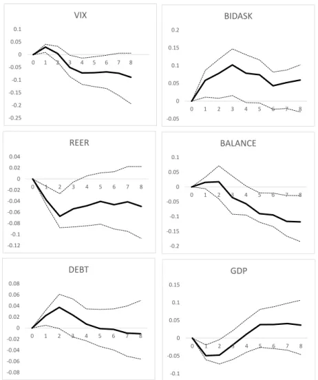
We plot in Figure 2 the spreads IRFs to the six main determinants, confirming that: i) an increases in the bid ask spread, VIX and debt differentials raise the spreads relative to Germany’s; ii) an improvement in the budget, higher growth prospects and exchange rate depreciation lower the spreads relative to Germany’s.

Table 1 shows the variance decomposition of the variables included in this first system. It is visible that the variance of spreads is essentially explained by itself. However, both the bid ask spreads and budget balance expectation differentials seem to play a non-negligible role (in bold).

[Table 1] [Figure 2]

Turning to the second system where we replace the budget balance with one budgetary component at a time, the spreads’ IRFs are displayed in Figure 3. Focus first on the black lines that cover the entire time span. On the expenditure side, a rise in either public wages or in social expenditure seems to increase spreads, whereas the effect is not statistically different from zero in the cases of public consumption, subsidies and public investment. On the revenue side, while a rise in social security contributions does not seem to greatly affect spreads, increases in both direct and indirect taxes, by improving the overall fiscal position, seem to lower the spreads differential. Table 2 presents the spreads’ variance decomposition of each PVAR corresponding to relevant budgetary variables. The variance of spreads remains essentially explained by itself, but indirect taxes can account for up to 2.5% after 16 quarters.

[Figure 3] [Table 2]

Interestingly, when we limit the sample to the post-2007Q3 period (corresponding to the start of the global financial crisis), we get a slightly different picture in the IRFs (see red lines in Figure 3). First, bear in mind that between 2008 and 2010 the countries in our sample underwent fiscal expansions to counter-act the negative effects of the recession.

We observe that a rise in all expenditure components (with the exception of subsidies) led to an increase in spreads, particularly social expenditure (used to compensate loss of income from unemployment). Taxes and social security contributions were lowered during this period which triggered an adverse perception from markets and the inevitable increase in spreads. From the point of view of fiscal policy the requirement of credibility comes down to its long-term sustainability and fiscal solvency condition for it is this that the capacity of a government to meet its long term liabilities depends upon. Alesina and Perotti (1996) assuming that a credible fiscal policy leads to lower spreads concluded that such policy is founded on control of expenditure and not on an extraordinary growth of revenue.

6 5. Conclusion

With a PVAR approach for 10 Euro area countries we find that: i) increases in the bid ask spread, VIX and debt raise the spreads relative to Germany’s; ii) improvements in the budget balance, higher growth and exchange rate depreciation lower them.

Moreover, rises in public wages or in social expenditure increase spreads, while increases in direct and indirect taxes lower them. In the post-2007Q3 period rises in all expenditure components (except subsidies) increased spreads.

References

Alesina, A., Perotti (1006), “Fiscal discipline and the budget process” American Economic

Review, 86(2).

Ardagna, S., Caselli, F., Lane, T. (2007). “Fiscal Discipline and the Cost of Public Debt Service: Some Estimates for OECD Countries”. The B.E. Journal of Macroeconomics, 7 (1).

Barrios, S., Iversen, P., Lewandowska, M., Setzer, R. (2009). “Determinants of intra-euro-area government bond spreads during the financial crisis”. European Commission, Economic Papers 388.

Bernoth, K., von Hagen, J., Schuknecht, L. (2012). “Sovereign risk premia in the European government bond market”. Journal of International Money and Finance, 31, 975-995.

Codogno, L., Favero, C., Missale, A. (2003). “Yield spreads on EMU government bonds.”

Economic Policy, 18, 211-235.

Ejsing, J., W. Lemke and E. Margaritov (2011). Sovereign Bond Spreads and Fiscal Fundamentals - a Real-Time, Mixed-Frequency Approach. Mimeo, ECB.

Favero, C., Pagano, M., von Thadden, E.-L. (2010). “How does liquidity affect government bond yields?” Journal of Financial and Quantitative Analysis, 45, 107-134.

Gerlach, S., Schulz, A., Wolff, G. (2010). “Banking and sovereign risk in the euro-area”. CEPR Discussion Paper No. 7833.

Kneller, R., Bleaney, M., Gemmell, N. (1999) "Fiscal policy and growth: evidence from OECD countries", Journal of Public Economics 74, 171-190.

Longstaff, F., Pan, J., Pedersen, L., Singleton, K. (2011). “How Sovereign Is Sovereign Credit Risk?” American Economic Journal: Macroeconomics, 3, 75–103.

Manganelli, S., Wolswijk, G. (2009). “What drives spreads in the euro-area government bond market?” Economic Policy, 24, 191-240.

Romero de Avila, D., Strauch, R. (2008), “Public Finances and Long Term Growth in Europe. Evidence from a Panel Data Analysis”, European Journal of Political Economy, 24(1), 172-191.

Table 1: Variance Decomposition of PVAR – baseline

Response quarter spread vix bidask reer balance debt gdp spread 4 88.89% 0.92% 5.32% 2.37% 0.49% 0.65% 1.36% spread 8 87.91% 2.30% 3.50% 1.62% 3.46% 0.25% 0.95% spread 12 88.02% 2.93% 2.95% 1.13% 4.29% 0.09% 0.59% spread 16 86.87% 3.47% 2.68% 1.01% 5.40% 0.05% 0.53% spread 20 86.59% 3.64% 2.58% 0.93% 5.75% 0.04% 0.46%

Note: percentage of variation in the row variable explained by column variable. In bold is marked the determinant with the greatest explanatory power by horizon and excluding spread.

Table 2: Variance Decomposition of PVAR - with budgetary components one at a time Response Budgetary component/quarter 4 8 12 16 20 Spread _{pecons 0.27% 0.35% 0.25% 0.24% 0.22%} Spread _{peemp 0.47% 0.77% 0.78% 0.86% 0.86%} Spread _{pesoc 0.39% 0.76% 0.84% 0.95% 0.97%} Spread _{pesub 0.02% 0.03% 0.08% 0.11% 0.13%} Spread _{peinv 0.18% 0.07% 0.02% 0.01% 0.00%} Spread _{prdirtax 0.18% 0.99% 1.24% 1.49% 1.51%} Spread _{prindtax 0.80% 2.00% 2.25% 2.52% 2.52%} Spread _{prsoc 0.03% 0.05% 0.03% 0.03% 0.03%}

Note: percentage of variation in spreads explained by corresponding budgetary component. In bold is marked the determinant with the greatest explanatory power by horizon and excluding spread.

Figure 1: 10-year government bond yield spreads (differential versus Germany)

0 5 10 15 20 25 1999Q1 2000Q1 2001Q1 2002Q1 2003Q1 2004Q1 2005Q1 2006Q1 2007Q1 2008Q1 2009Q1 2010Q1 2011Q1 2012Q1

belgium greece spain france ireland italy netherlands austria portugal finland

8

Figure 2: Spreads IRFs to shocks in fundamental determinants

-0.25 -0.2 -0.15 -0.1 -0.05 0 0.05 0.1 0 1 2 3 4 5 6 7 8 VIX -0.05 0 0.05 0.1 0.15 0.2 0 1 2 3 4 5 6 7 8 BIDASK -0.12 -0.1 -0.08 -0.06 -0.04 -0.02 0 0.02 0.04 0 1 2 3 4 5 6 7 8 REER -0.2 -0.15 -0.1 -0.05 0 0.05 0.1 0 1 2 3 4 5 6 7 8 BALANCE -0.08 -0.06 -0.04 -0.02 0 0.02 0.04 0.06 0.08 0 1 2 3 4 5 6 7 8 DEBT -0.1 -0.05 0 0.05 0.1 0.15 0 1 2 3 4 5 6 7 8 GDP

Figure 3: Spread impulse responses to shocks in budgetary determinants: full sample and Global Financial Crisis period

-0.2 -0.15 -0.1 -0.05 0 0.05 0.1 0.15 1 2 3 4 5 6 7 8 9 GOV CONSUMPTION -0.2 -0.15 -0.1 -0.05 0 0.05 0.1 0.15 1 2 3 4 5 6 7 8 9 PUBLIC WAGES -0.2 -0.15 -0.1 -0.05 0 0.05 0.1 0.15 1 2 3 4 5 6 7 8 9 SOCIAL EXPENDITURE -0.2 -0.15 -0.1 -0.05 0 0.05 0.1 0.15 0 1 2 3 4 5 6 7 8 SUBSIDIES -0.2 -0.15 -0.1 -0.05 0 0.05 0.1 0.15 0 1 2 3 4 5 6 7 8 PUBLIC INVESTMENT -0.2 -0.15 -0.1 -0.05 0 0.05 0.1 0.15 0 1 2 3 4 5 6 7 8 DIRECT TAXES -0.2 -0.15 -0.1 -0.05 0 0.05 0.1 0.15 0 1 2 3 4 5 6 7 8 INDIRECT TAXES -0.2 -0.15 -0.1 -0.05 0 0.05 0.1 0.15 0 1 2 3 4 5 6 7 8 SOCIAL SECURITY CONTRIBUTIONS

Note: Errors are 5% on each side generated by Monte-Carlo with 500 replications. Black lines correspond to the entire time span, whereas red lines correspond to the global financial crisis period, i.e., from 2007Q3 onwards.