Joana Isabel Faustino Martins
Bachelor of Science in Biomedical EngineeringBrain Plasticity associated with
Predictive Masking and Glaucoma
Dissertation submitted in partial fulfillment of the requirements for the degree of
Master of Science in Biomedical Engineering
Adviser: Frans W. Cornelissen, Professor, University Medical Center Groningen Co-adviser: Ricardo Vigário, Auxiliar Professor, NOVA
University of Lisbon
Examination Committee Chairperson: Prof. Dr. Carla Maria Quintão Pereira
Raporteur: Prof. Dr. Maria João Gomes Trindade Caseiro
Brain Plasticity associated with Predictive Masking and Glaucoma
Copyright © Joana Isabel Faustino Martins, Faculty of Sciences and Technology, NOVA University Lisbon.
The Faculty of Sciences and Technology and the NOVA University Lisbon have the right, perpetual and without geographical boundaries, to file and publish this dissertation through printed copies reproduced on paper or on digital form, or by any other means known or that may be invented, and to disseminate through scientific repositories and admit its copying and distribution for non-commercial, educational or research purposes, as long as credit is given to the author and editor.
Ac k n o w l e d g e m e n t s
First and foremost, I would like to thank the institution that was my second home dur-ing the last five years, FCT-NOVA. In particular to Prof. Dr. Carla Quintão, coordinator of the master in Biomedical Engineering, for the excellent work and devotion to raising teaching conditions, as well as giving response and voice to the students.
To my adviser Prof. Dr. Frans Cornelissen for the opportunity to have worked on such a fascinating project. Thank you for the trust, availability, motivation and appreciation to my work during our meetings.
To that person who was my cornerstone during this first introduction to the scientific research world, Joana Carvalho. Thank you for the contagious passion for science but most of all, for the long hours of work side by side, the moments of joy as well as those of greater frustration. You were an exceptional guide, and I think I am allowed to say that we made a good team. This thesis reflects everything you have taught me.
The work of scientific research is teamwork. In this sense, I would like to thank Azzurra Invernizzi for sharing your knowledge with me and believing in my potential. To my dear colleague Alessandro Grillini for his wise advice, not only academic but also personal. To Shereif Haykal, Rijul Soans, Hinke Halbertsma and Birte Gestefeld for the sympathy and welcoming me to the group.
To my co-adviser Prof. Dr. Ricardo Vigário for allowing me to pursued and develop my thesis project abroad.
My journey at FCT-NOVA started in a somewhat turbulent way. Life has taught me to always look to the bright side, even in the most unpleasant situations. Words will never be enough to thank all the support and affection I had received by the time when no one knew me well. To all my college friends, I am forever grateful that you made me feel that I belonged to something when I saw my world crumble. In particular, I would like to thank a group of people that I want to take with me outside the doors of this institution: Beatriz Costa, Ana Sousa, Ana Pinheiro, Joana Inácio, Inês Dias, João Narciso, Bruno Meireles, Sara Santos, Maria Inês Correia, Miguel Santos and João Tavares.
At last, to the four people in my life that I want to make the most proud of me. To my mother, for never letting me give up and always being there for me. To my father, who always supports my decisions even if they imply being physically away from him. To my aunt, my second mother, for striving to see me happy. And to my sister, my reference, for the friendship and for teaching me what it means to be a great woman.
A b s t r a c t
Glaucoma is a disease resulting from damage at the optic nerve, the “highway” through which visual information travels from the retina towards the visual brain. Such lesion deprives the visual cortex of the regular input, causing interruptions within the visual field – scotoma. However, even when such lesions occur, perception remains stable as the human visual system perceptually masks the insult with the visual features of nearby regions of the visual field. To unravel the neural mechanisms by which this remarkable capacity occurs in glaucomatous individuals, we used functional magnetic resonance imaging (fMRI) and neural modelling to track changes in cortical population receptive fields (pRFs). We found that visual neurons from early visual areas (V1-3) expanded their pRFs both inside and at the vicinity of the lesion. V1 pRFs also shifted their preferred central position towards the outside of the scotoma. By doing so, neural populations were able to process information from spared visual field, consistent with the notion of predictive masking. In contrast, well-sighted observers did not show similar patterns of neural activity in response to the introduction of an artificial scotoma (AS). Our findings provide evidence of enduring cortical reorganization underlying the predictive spatial masking of scotomas in glaucoma, meeting the contemporary view that early visual areas of the adult human brain retain plastic mechanisms. Furthermore, the involvement of the brain suggests that glaucoma pathogenesis goes beyond the eye.
R e s u m o
O Glaucoma resulta de uma lesão ao nível do nervo ótico, a “estrada” através da qual a informação visual viaja da retina em direção ao cérebro. Tal dano priva o córtex visual do input esperado o que, por sua vez, gera interrupções no campo visual – escotomas. No entanto, mesmo quando essas lesões ocorrem, a capacidade de percepção visual per-manece estável uma vez que, o sistem visual humano tem a capacidade de mascarar a lacuna de informação com as características do campo visual circundante. De forma a des-mistificar os mecanismos neuronais através dos quais esta capacidade notável ocorre em indíviduos diagnosticados com glaucoma, utilizou-se ressonância magnética functional (fMRI) e modelagem neuronal de forma a investigar alterações nas populações de campos receptivos corticais (pRFs). Observou-se que os neurónios visuais alocados nas áreas vi-suais primárias (V1-3) expandiram os seus pRFs tanto dentro, com nas proximidades do escotoma. Adicionalmente, os pRFs correspondentes à área V1 reconfiguraram sua posi-ção espacial, deslocando o seu centro para o exterior da lesão. Desta forma, as populações neuronais foram capazes de processar informação de regiões intactas do campo visual, o que está de acordo com a noção de mascaramento preditivo. Em contraste, observadores com visão normal (ou corrigida para normal) não revelaram tais padrões de atividade neuronal aquando da visualização de um estímulo com um escotoma artificial sobreposto. Os resultados acima mencionados fornecem evidências de uma reorganização cortical duradoura subjacente ao mascaramento preditivo de escotomas na doença do glaucoma, atendendo à visão contemporânea de que as áreas visuais primárias do cérebro humano retêm plasticidade. Além disso, o envolvimento do cérebro sugere que a patogénese do glaucoma não se limita aos efeitos oculares.
Palavras-chave: glaucoma, mascaramento preditivo visual, campo receptivo populacio-nal, reorganização cortical, fMRI
C o n t e n t s
List of Figures xvii
List of Tables xxi
Acronyms xxiii
1 Introduction 1
1.1 Outline of the thesis . . . 2
2 Human Visual System 5 2.1 The Eye . . . 5
2.2 Neuronal Pathways . . . 6
2.3 The Visual Cortex . . . 9
2.3.1 Functional Areas in the Visual Cortex . . . 9
2.3.2 Retinotopic Organization of the Visual Cortex . . . 11
3 Visual Field Defects 13 3.1 The Normal Visual Field . . . 13
3.2 Glaucoma . . . 14
4 Visual Field Defects and The Brain 17 4.1 Brain Plasticity . . . 17
4.2 Predictive Masking . . . 18
5 Functional Magnetic Resonance Imaging 21 5.1 The BOLD Signal . . . 21
6 Visual Field Mapping 25 7 Population Receptive Field (pRF) Changes in Opthalmic and Neurologic Dis-eases: State-of-the-Art 29 8 Materials and Methods 33 8.1 Study Design and Population . . . 33
8.3 Visual Stimulation . . . 38
8.3.1 Stimulus Presentation . . . 38
8.3.2 Stimulus Description . . . 38
8.4 Magnetic Resonance Imaging . . . 40
8.4.1 Scanning . . . 40
8.4.2 Experimental Procedure . . . 40
8.5 Data Preprocessing . . . 42
8.5.1 Preprocessing of Anatomical Images . . . 42
8.5.2 Preprocessing of Functional Images . . . 45
8.6 Data Analysis . . . 46
8.6.1 Population Receptive Field Mapping . . . 46
8.6.2 Regions-of-Interest Definition . . . 48
8.6.3 Visual Field Coverage Map . . . 48
8.6.4 Scotoma Projection Zone (SPZ) Definition . . . 53
8.6.5 Statistical Analyses . . . 55
9 Results 57 9.1 Changes in BOLD signals . . . 58
9.2 Visual Field Maps and pRF Properties . . . 59
9.2.1 Enlargement of pRFs in glaucoma . . . 63
9.2.2 pRF size as a predictor of disease severity . . . 65
9.2.3 Position reconfiguration of pRFs in glaucoma . . . 66
9.3 Correspondence between visual field coverage maps and perimetric sco-tomas . . . 68
10 Discussion 73 10.1 Overall decreased neural activity in the visual cortex of glaucoma patients 73 10.2 Retinotopic Remapping in the visual cortex in glaucoma . . . 74
10.2.1 Rescaling and displacement of neuronal populations underly PM of scotomas in glaucoma . . . 74
10.2.2 Does pRF size correlate with glaucoma severity? . . . 76
10.3 Visual Field Coverage Maps versus Clinical Measures . . . 77
11 Conclusions and Future Work 79 11.1 Limitations . . . 80
11.2 Future Research and Applications . . . 82
Bibliography 85 A Supplementary Material 97 A.1 Visual Field Maps . . . 97
C O N T E N T S
I Magnetic Resonance Imaging Principles 103
I.1 Pulse sequence . . . 106 I.2 Image Contrast . . . 107
L i s t o f F i g u r e s
2.1 Schematic anatomy of the eye . . . 6
2.2 Diagram of the organization of the retina and distribution of photoreceptors 7 2.3 Schematic drawing of the human optic pathway . . . 8
2.4 The arrangement of visual processing framework . . . 10
2.5 Visual field representation in the primary visual cortex (V1) . . . 11
3.1 The normal visual field . . . 14
3.2 Ocular damage in primary POAG and PACG . . . 15
3.3 Healthy versus glaucomatous vision . . . 16
4.1 Filling-in at the blind-spot . . . 19
5.1 Illustration of a hemodynamic response evoked by neuronal activity in re-sponse to a hypothetical brief stimulus (red bar) . . . 22
6.1 Traveling Wave Retinotopy (TWR) . . . 26
6.2 The population receptive field (pRF) modeling pipeline . . . 27
8.1 Flow diagram of the study . . . 35
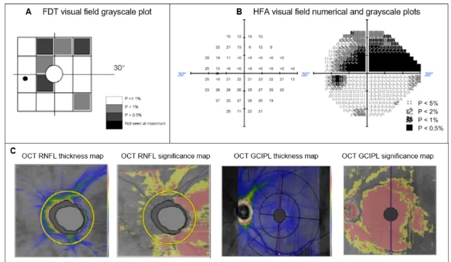
8.2 Examples of ophthalmic evaluations’ outcomes . . . 37
8.3 Example of the stimuli used to obtain pRF parameter estimates . . . 39
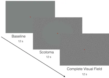
8.4 Example of the stimuli used to obtain the location of the scotoma projection zone (SPZ) . . . 40
8.5 Example of AC/PC alignment . . . 43
8.6 Example of segmented GM and WM of an axial (left), coronal (middle) and sagittal (right) brain slices . . . 44
8.7 Example of a three-dimensional surface constructed using mrMesh . . . 45
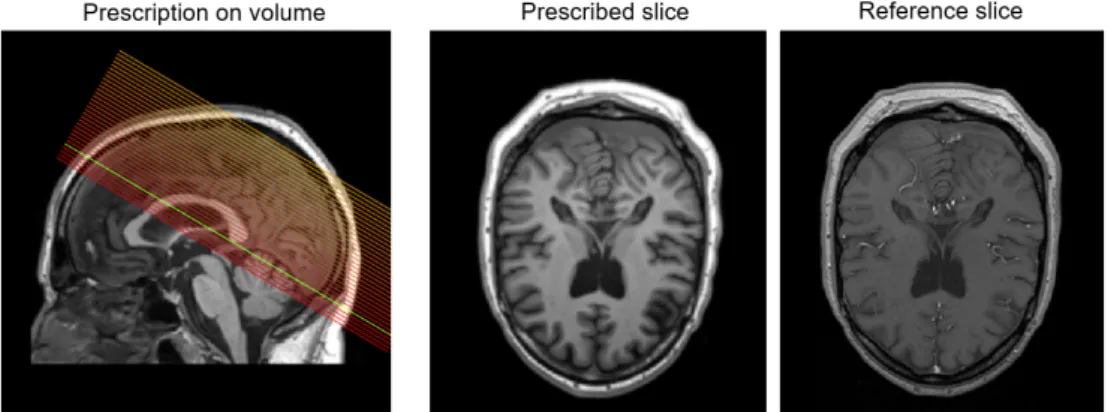
8.8 The result of the alignment of the inplane anatomy to the full volume . . . . 46
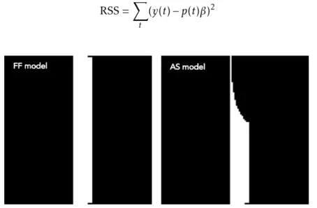
8.9 The full field (FF) (left) and artificial scotoma (AS) (right) model used in the pRF analysis . . . 47
8.10 Visualization of polar angle estimates on left and right cortical hemispheres and definition of ROIs . . . 48
8.11 pRF-based V1 coverage map framework . . . 50
8.13 Definition of the SPZ based on the localizer . . . 54 8.14 V1 coverage map for a glaucomatous subject with HFA numerical grid overlaid 55
9.1 Standard deviation of the mean time series (in arbitrary units) for 3 different ROIs for patients (red) and controls with and without AS (light and dark blue, respectively) . . . 59 9.2 Visualization of VFM based estimates using pRF for a glaucomatous subject
and the age-matched control obtained with a luminance-contrast defined stim-uli . . . 60 9.3 Average voxel-wise pRF size plotted as a function of pRF eccentricity for 3
different ROIs . . . 61 9.4 Average voxel-wise pRF size plotted as a function of explained variance (EV)
for 3 different ROIs . . . 62 9.5 Comparison of voxel-wise eccentricity for masked and unmasked visual field
in the control population and, for monocular and binocular performance in the glaucoma population, for 3 different ROIs . . . 63 9.6 Quantitative comparison of cumulative percentage of pRF size for glaucoma
and control groups . . . 64 9.7 Differences of pRF size across delineated regions of the visual field and visual
areas . . . 65 9.8 The relationship between pRF size and ophthalmic perimetric evaluation in
visual areas V1-V3 . . . 66 9.9 pRF center distribution as a function of distance from the fovea . . . 68 9.10 Comparison between perimetric outcome measures and visual field coverage
maps . . . 70 9.11 Comparison between perimetric outcome measures and visual field coverage
maps . . . 71
A.1 Visualization of VFM based estimates using pRF for a P10 and the age-matched control obtained with a luminance-contrast defined stimuli . . . 97 A.2 Visualization of VFM based estimates using pRF for a P12 and the age-matched
control obtained with a luminance-contrast defined stimuli . . . 98 A.3 Visualization of VFM based estimates using pRF for a P17 and the age-matched
control obtained with a luminance-contrast defined stimuli . . . 98 A.4 Visualization of VFM based estimates using pRF for a P18 and the age-matched
control obtained with a luminance-contrast defined stimuli . . . 99 A.5 Visualization of VFM based estimates using pRF for a P12 and the age-matched
control obtained with a luminance-contrast defined stimuli . . . 100 A.6 Comparison between perimetric outcome measures and visual field coverage
L i s t o f F i g u r e s
A.7 Comparison between perimetric outcome measures and visual field coverage maps of P18 and aged-matched control . . . 101
I.1 MRI physics . . . 104 I.2 Application of radio frequency pulse (RF) and relaxation times . . . 106 I.3 The importance of correctly setting repetition time and echo time to obtain T1
L i s t o f Ta b l e s
8.1 Summary of group-dependent inclusion criteria . . . 34
8.2 MRI protocol for the glaucoma participants . . . 41
8.3 MRI protocol for the control participants . . . 42
9.1 Summary of glaucoma participants in the study . . . 58
9.2 Statistical analysis of the relation between pRF size and explained variance . 61 9.3 Statistical analysis of the relationship between pRF size and average mean deviation (MD) score in visual areas V1-V3 . . . 66
Ac r o n y m s
AC Anterior Commissure.
AS Artificial Scotoma.
BOLD Blood-oxygen-level-dependent.
CSF Cerebrospinal Fluid.
DWI Diffusion Weighted Imaging. EV Explained Variance.
FDT Frequency Doubling Perimetry.
FF Full Field.
fMRI functional Magnetic Resonance Imaging.
FOV Field-of-view.
GLM General Linear Model.
GM Gray Matter.
HFA Humphrey Field Analiser.
HRF Hemodynamic Response Function.
HTG High-Tension Glaucoma.
IOP Intraocular Pressure.
LCR Luminance-contrast defined retinotopy.
LGN Lateral Geniculate Nucleus.
LPZ Lesion Projection Zone.
LTI Linear Time-Invariant.
MD Mean Deviation.
MP Micro Probing.
MR Magnetic Resonance.
MRI Magnetic Resonance Imaging.
NCDF Normal Cumulative Distribution Function.
NCT Non-contact Tonometry.
NTG Normal-Tension Glaucoma.
OCT Optical Coherence Tomography.
ON Optic Nerve.
ONH Optic Nerve Head.
PACG Primary Angle-Closure Glaucoma.
PC Posterior Commissure.
PM Predictive Masking.
POAG Primary Open-Angle Glaucoma.
pRF Population Receptive Field.
RF Receptive Field.
RGC Retinal Ganglion Cell.
RNFL Retinal Nerve Fiber Layer.
ROI Region-of-interest.
RPE Retinal Pigment Epithelium.
RSS Residual Sum of Squares.
SD Standard Deviation.
SNR Signal-to-noise ratio.
SPZ Scotoma Projection Zone.
TE Echo Time.
TR Repetition Time.
AC R O N Y M S
VA Visual Acuity.
VF Visual Field.
C
h
a
p
t
e
r
1
I n t r o d u c t i o n
Glaucoma is one of the leading causes of blindness worldwide that is predicted to affect 112 million people by the year 2040 [1]. Described as a collection of neurodegenerative diseases, glaucoma is caused by an initial loss of retinal ganglion cells (RGCs) accompa-nied by the progressive damage of the optic nerve. This results in regions of deprived visual input - scotomas - within the visual field of the affected eye. Although glaucoma is traditionally considered an eye disease, there is increasing evidence that its neurode-generative effects are not restricted to the retina and optic nerve, instead spreading along the entire length of the visual pathway towards the brain [2–5].
Even though glaucoma may cause irreversible blindness, it can be prevented if di-agnosed early. Nevertheless, the disease frequently goes unnoticed as individuals with scotoma often do not realize that such damage exists until an objective ophthalmic test is performed. This is because predictive masking (PM), also referred to as filling-in, occurs at the scotoma whereby the visual cortex predicts and interpolates the missing visual fea-tures, such as color, brightness, texture, and motion, of the incomplete scene [6]. Despite its scientific and clinical relevance, the underlying neuronal mechanisms of PM are still ill-understood.
Previous studies that probe PM and examination of the neural impact of retinal lesions have shown that the brain reorganizes through re-scaling and displacement of the recep-tive fields towards spared regions of the visual field [7–10]. The receprecep-tive field (RF) of a visual neuron refers to the portion of the visual field that is most effective at driving the neuron’s response. Estimating the RF of visual neurons is therefore of great importance in the investigation of how the visual brain responds to a damage in the visual system. Since recently, there is a debate about whether the ‘ectopic’ RFs - altered in position and/or size - should actually be interpreted as evidence of cortical reorganization because the same
Hence the changes in the RFs will have an impact in the functional organization of the visual cortex. A common way to assess the correspondence between visually selective neurons and their RFs in visual space is to systematically stimulate certain parts of the visual field while monitoring the neuronal stimulus-evoked responses with functional magnetic resonance imaging (fMRI) [14–16]. This is called visual field mapping because due to the retinotopic organization of the visual cortex (i.e. nearby visual neurons respond to nearby locations in the visual field) it is possible to unravel a number of different visual field maps. Nowadays, with the urge of neurocomputational models, such as population receptive field (pRF) [17], it is possible to use visual field mapping data to estimate properties of the RFs of visual neurons which is useful when it comes to investigating cortical reorganization.
The plasticity (reorganization) of the visual cortex during PM has not been studied in particular. Adding to this, despite the large number of studies about cortical reorga-nization using fMRI visual field mapping methods, most of them have addressed central visual disorders. In glaucoma, visual field loss starts peripherally and so the mechanisms of spatial reorganization might be different from those where central vision degenerates, given that peripheral and central vision are distinctly processed in the cortex [18].
Based on the above statements, in the present study, we sought to determine the neuronal mechanism underlying the PM of scotomas in glaucoma. We hypothesize that there is a reorganization of the visual cortex, evident from an enlargement of the RFs surrounding the scotomas, and a shift towards the edges of the scotoma. To test our hypothesis, we used fMRI in combination with biologically inspired neural population receptive modeling (pRF) to track changes in RFs’ properties of a glaucoma population. Moreover, we delineated visual field coverage maps from the pRF characteristics and based on a novel methodology to depict the visual field defects. We contrasted the results with those of healthy well-sighted controls in whom the lesions of the glaucoma visual system were mimicked through introduction of an artificial scotoma (AS) into their visual field.
1.1
Outline of the thesis
This thesis is organized in 11 chapters. The present one serves to reveal and explain the underlying research question, as what is hypothesized to be found and the means to address it.
In chapter 2 there is an overview of the human visual system, from the very beginning of visual processing in the eye to the complexity of the visual areas in the brain.
Chapter 3 includes a description of a standard visual field, as well the defects to the visual field arising from damage to the optic nerve in the case of the disease in focus – Glaucoma. A description of glaucoma pathophysiology is additionally presented.
Following the theme of chapter 3, in chapter 4 it is described the effects of visual field defects in the brain, including mechanisms of neuroplasticity and the perceptual
1 . 1 . O U T L I N E O F T H E T H E S I S
phenomenon of PM.
Chapter 5 reveals the principles of fMRI, in particular the haemodynamics that un-derly neuronal activity following stimulation. As this thesis revolves around evaluating visual field maps in the human brain, chapter 6 reveals a brief introduction of the tech-nique used to do so by means of a combination of fMRI and visual stimulation: the pRF approach.
We also reviewed the literature on pRF changes in ophthalmic and neurologic diseases (chapter 7), to give an insight into the current state of pRF as a way to reveal cortical reorganization.
Chapter 8 includes the methods that were used to determine the organization of the visual cortex of the participants of the study. In chapter 9 and 10, the results are gathered together and discussed, respectively.
At last, chapter 11 presents the main findings and limitations of this study. Addition-ally, it includes some suggestions for future work and improvements.
A supplementary material chapter is presented at the end of the document which contains a group of results not shown in the main results chapter. The principles under-lying Magnetic Resonance Imaging (MRI) as well as a resume about the General Linear Model (GLM) are included as annexes due to their relevance to the understanding of the methodology used in this thesis.
C
h
a
p
t
e
r
2
Hu m a n Vi s ua l S y s t e m
Sight underlies the ability to understand the world and to navigate within the surround-ing environment. As one looks around, the eyes are continually absorbsurround-ing light rays that are essential to the visual process. The light travels deep into the eyeballs towards the back of each of them where its energy is transformed into electrical impulses. These impulses are carried on to the visual cortex, along neuronal pathways, where they are ultimately processed and unified into a single image.
The eye together with the conducting paths, that carry the visual information, and the visual receiving brain areas form a compact unit – the visual system.
2.1
The Eye
The eye consists of a complex sensory organ that plays a fundamental role in visual perception, one of the essential human senses.
Visual information enters the eye through the cornea, the transparent front “window” of the eye, that due to its curvature enables most of the eye’s focusing power. The cornea is anteriorly nourished with oxygen by tears and posteriorly bathed by a clear liquid called aqueous humor, which sustains the shape of the eyeball [19].
The cornea’s refractive power bends the light rays enabling them to freely pass through the pupil, a hole allocated in the center of the iris. The iris controls the pupil size by contracting and expanding, hence, defining the level of illumination onto the retina.
Once through the gate of the pupil, the visual information reaches the lens where the remainder focusing ability is provided helping the eye to see sharply both near and far, a phenomenon calledaccommodation [20]. The lens focuses the light through the vitreous
humor, a gel-like substance that fills the space between the lens and the retina, forming an upside-down image which is projected onto the retina [19].
The retina is a complex nervous tissue that covers two-thirds of the back of the eyeball [19]. By converting the light signals into electrical impulses, the retina represents the starting-point of the visual pathways.
Figure 2.1: Schematic anatomy of the eye. Reprinted from [21].
2.2
Neuronal Pathways
The visual processing starts in the retina. Anatomically the retina is composed of ten layers. However, these ten layers are commonly grouped into four main ones (Figure 2.2A): (1) the retinal pigment epithelium (RPE), the outermost layer above which are (2) the photoreceptors; which convert light into a neuronal (electric) signal and transmit it to (3) the bipolar cells which, in turn, are connected to the innermost layer of neurons, (4) the RGCs [22].
The RPE is a darkly pigmented layer that is not responsive to radiant energy and therefore plays no role in encoding visual information. It captures the photons which escape absorption by the photoreceptive layer. This is essential to prevent light scattering behind the retina necessary to high-contrast image [19].
By the time light reaches the photoreceptive layer, as the photopigment molecules of the photoreceptors react to light stimulus, it is absorbed and converted into electrical signals through a process known asphototransduction.
There are two kinds of photoreceptors, rods, and cones, that differ regarding structure, by their distinctive shapes, but mostly in function by their sensitivity to specific light wavelengths. Rods are the foundation of scotopic vision, i.e., vision at low luminance levels. On the other hand, cones mediate daytime vision, medium to high luminance lev-els, providing color perception and high spatial acuity. The cones are grouped into three
2 . 2 . N E U R O N A L PAT H WAY S
types depending on the wavelength sensitivity they react to: long (red light), medium (green light), or short (blue light) [19].
Rods and cones are not uniformly distributed throughout the retina as shown in Figure 2.2B. The highest density of cones is situated in the central part of the retina, known as the fovea. Thereby, the fovea encompasses a high-resolution zone, mediating detailed vision. Away from the fovea, cone density decreases sharply. The amount of rods increases, and finally declines in the most peripheral part of the retina [20].
Figure 2.2: Diagram of the organization of the retina and distribution of photorecep-tors. (A)The different types of cells and the variety of interconnections in the retina. The retina is vertically organized from the photoreceptors, on the top edge of the figure, to bipolar cells to retinal ganglion cells, on the lower edge. The vertical pathway of light is also mediated by horizontal organized cells, at the photoreceptor-bipolar synaptic layer, and amacrine cells, at the bipolar-ganglion cell synaptic layer. (B) The fovea contains the highest density of cones whereas in the peripheral retina rods predominate over cones. Note that are no receptors in the blind spot. Adapted from [20].
The electrical signals resulting from phototransduction set the beginning of the ver-tical pathway, a feedforward chain of synapses through the neuronal layers of the retina
[20]. The electrical signals travel from the photoreceptors, via the bipolar cells to the RGCs. In addition, horizontal and amacrine cells transmit information from a neuron in one layer to adjacent neurons in the same layer (Figure 2.2A).
There are distinct forms of RGCs. They are commonly classified into two broad categories based on their anatomical features, functions, and projections onto the lateral geniculate nucleus (LGN) in the thalamus: the parvocellular and magnocellular RGCs [23]. Parvocellular RGCs, or P-cells, are the most prevalent type (approximately 80% of the RGCs). Characterized by small cellular bodies, they concern with detail and are involved in processes such as object recognition and form representation [23]. As a group, these cells form the often calledparvocellular pathway as they project to the parvocellular
the RGCs and project to the magnocellular layers of the LGN, all together they form the so-called magnocellular pathway [23]. With larger cell bodies and dendritic arbors
compared to P-cells, M-cells operate quickly, however, with a lack of detail, dealing with the processing of object localisation and motion.
The axons of RGCs come together to form the optic nerve, which serves as a highway for the signals to reach the visual areas of the brain [20]. The expansion of the optic nerve fibers is called retinal nerve fiber layer (RNFL). The optic nerve leaves the eye at the optic disc, a location also called the blind spot, due to a complete absence of photoreceptors
(Figure 2.2B). Note that we are not consciously aware of this “blind spot”, as a result of PM (discussed in detail further in this thesis) [24].
The nerves from both eyes join to form the optic chiasm. At the optic chiasm, axons from RGCs from the nasal side of the retina cross over allowing each hemisphere of the brain to receive information from the opposite side of the visual scene. Information from the right visual field travels through the left optic tract towards the left hemisphere while information from the left visual field travels through the right optic tract towards the right hemisphere (Figure 2.3A) [20]. Each optic tract terminates in the LGN.
Figure 2.3: Schematic drawing of the human optic pathway. (A) The path of the visual information from the eyes towards the visual cortex through the right- (red) and left-hemispheric (blue) fiber pathways. (B) Right LGN projection to the right primary visual cortex. The LGN is made up of 6 layers. P-cells project to layers 3-6 whereas M-cells project to layers 1 and 2. The ipsilateral (I) and contralateral (C) project to alternate layers. Adapted from [25].
The LGN consists of a folded sheet of neurons cluster into six layers. The two inner layers (1 and 2) receive input from the M-cells, and the four outer remaining layers (3-6)
2 . 3 . T H E V I S UA L C O R T E X
receive input from the P-cells. Thus, information splits into two streams: the magnocel-lular pathway and the parvocelmagnocel-lular pathway. The ‘magno’ subdivision carries signals for motion detection, depth and flick whereas the ‘parvo’ subdivision deals with color vision, texture, shape and fine detail. The separation of the visual field information is conserved. Input from the ipsilateral eye terminates in layers 2, 3, and 5, and information from the contralateral eye in layers 1, 4 and 6 (Figure 2.3B) [26].
Although ‘magno’ and ‘parvo’ pathways are often described as parallel, that is only an approximation as there is actually interaction between them. This interaction allows various visual features (e.g., color, depth, form and motion) to be linked, resulting in unified visual percept. One way this linkage might be accomplished is through cells that are tuned to more than one feature [26].
After the LGN, the visual information travels through the optic radiations that ulti-mately project onto the visual cortex. Here, the information is integrated and processed to create an image to be perceived.
2.3
The Visual Cortex
2.3.1 Functional Areas in the Visual Cortex
The visual cortex is the ultimate stage of the visual system where the visual information is processed, and thus a synthesized image is generated. In humans, the visual cortex occupies approximately 20% of the cerebral cortex [27] and includes the entire occipital lobe (at the back of the skull), extending significantly into the temporal and parietal lobes (Figure 2.4A). It comprises 4-6 billion neurons [28].
Visual neurons are tuned to different features of the visual scene, such as color, motion, orientation, texture, shape, and depth. All these features are analyzed in parallel by separate specialized areas. Distinct cortical areas involved in visual processing have been identified in the macaque monkey [29]. With the evolution of non-invasive neuroimaging techniques, particularly fMRI, several visual areas have been recognised in the human as well [27].
V1 is the first visual area to allocate the visual input from the retino-geniculate (i.e., retina to LGN) pathway, reason why it is also known as the “primary visual cortex”. Additionally, it is where the information from both eyes is first combined. Area V1 lies posteriorly in the occipital lobe and concentrates within the calcarine sulcus, which can be found on the medial surface of both hemispheres (Figure 2.4A). The intrinsic circuitry of V1 is organized into a layered structure. In Figure 2.4B a cross section of V1 shows six major layers. The principal input comes from both already mentioned ‘magno’ and ‘parvo’ pathways (section 2.2) and is allocated by layer 4. From there the visual information is processed over a complex and specific sequence of interlaminar connections. Briefly, the most superficial layers (1, 2 and 3) receive information from layer 4 and then send the outputs to higher-order areas, whereas layers 5 and 6 project onto non cortical areas, such
as the LGN and the superior colliculus (a structure in the midbrain), respectively. [26]. Information processing up to the V1 is conventionally termed as lower-level processing, responding to simple properties such as orientation and spatial frequency. Beyond V1, increasingly complex features are processed sequentially by higher visual areas.
Information from V1 towards the rest of the brain flows along two main streams each serving a different function in visual information processing: the ventral and the dorsal stream (Figure 2.4A). Along these two streams size, latency, and complexity of the receptive fields increase. The ventral stream, or “what” pathway, is associated with object perception and recognition. Damage to this stream produces impairments on object discrimination tasks. In contrast, the dorsal stream, or “where” pathway, concerns with object localization, spatial awareness, and movement detection. Damage to this stream does impair performance on visuospatial tasks. V1 projects the ventral stream to the temporal lobes and the dorsal stream to the parietal lobes (Figure 2.4A) [26].
Figure 2.4: The arrangement of visual processing framework. (A) Information spill out of the retina to the primary visual cortex through the LGN. After the information arrives at V1, visual processing proceeds in two distinct pathways: dorsal pathway (blue) and ventral pathway (red). (B) V1 is segregated into six major layers The outputs are sent to higher cortical areas, back to the LGN and other subcortical nuclei. Adapted from [26].
The dorsal pathway flows from V1 and first to its adjacent visual area V2. V2, similarly to V1, responds to simple features such as orientation, spatial frequency, and color, but is also modulated by attention and more complex patterns. Then, visual information is received by area V3 and subsequently by V5 (or MT, middle temporal area) that are believed to be sensitive to visual motion and stereoscopic depth [30]. On the other hand, the ventral pathway flows into V1 to V2, V3 and lastly to V4 (Figure 2.4A).
It has been suggested that the ventral and dorsal stream can be traced back to the two principal cytological subdivisions of the RGCs: the parvocellular and magnocellular pathway. In fact, the ‘parvo’ pathway, with information about color and shape, would seem ideal for the ‘what’ pathway. Likewise, once dealing with motion information, the ‘magno’ pathway would seem to be the obvious candidate for the ‘where’ pathway. There’s evidence, however, that both dorsal and ventral streams communicate, receiving input
2 . 3 . T H E V I S UA L C O R T E X
from both ‘magno’ and ‘parvo’ pathways [31]. As an approximation the dorsal pathway is said to be magno-dominated and the ventral pathway to be parvo-dominated [32].
2.3.2 Retinotopic Organization of the Visual Cortex
Shaped by evolutionary and developmental constraints, the anatomical circuitry of the human sensory cortices follows the topographic organization of their corresponding sen-sory surfaces. In the case of the visual system, the mapping of the observed image onto the cortex results from the gathering of the RFs of individual neurons. A fundamental characteristic of the visual cortex is its ability to preserve the image’s spatial relationships formed in the retina, i.e., nearby portions of the visual field are processed by neighbour-ing visual neurons [33] (Figure 2.5). Hence, visual areas are said to follow a retinotopic organization.
Figure 2.5: Visual field representation in the primary visual cortex (V1). The polar-coordinates axes, eccentricity and polar angle, are identified on the visual field on the left panel. The black circle corresponds to the centre of the visual field (fovea). On the right panel the left visual field is represented on a zoom-in figure of the calcarine sulcus, where V1 falls in, of an unfolded cortical representation. Note that there is more cortical area devoted to the representation of the central part compared to more peripheral regions of the visual field - cortical magnification [34]. Reprinted from [35]
The human visual pathways map the visual image from cartesian coordinates in the visual field to polar coordinates in cortex. As one moves along the cortical surface from a posterior to an anterior position in the visual cortex, the representation of the visual field smoothly shifts from the center (fovea) to the periphery (Figure 2.5). This is called
eccentricity. RFs size is known to vary with eccentricity [26]. The fovea, where the
reso-lution is highest, encompasses the smallest RFs. RFs become progressively larger with distance from the fovea. Along with eccentricity, to identify a unique location in visual space there is another dimension needed - thepolar angle(Figure 2.5).
The type of representation illustrated by the previously described polar dimensions can be found in various visual areas, namely V1, V2, and V3, that as a group forms the
so-called early visual cortex (or early visual areas). The underlying research on this thesis focused on these three areas.
Per hemisphere, the topographic organization of V1 accommodates the representation of half of the visual field (a hemifield) with a contiguous polar angle and eccentricity (Figure 2.5). A larger portion of cortex is dedicated to the fovea than to the periphery - cortical magnification (Figure 2.5) [34]. This phenomenon is the reason why we see sharper in the fovea than in the periphery. The nearby visual field maps V2 and V3 cluster around V1, sustaining parallel eccentricity representations. However, in contrast to V1, these maps are discontinuous resulting in split-hemifield representations, i.e., quarterfinals, characterized by reversals in polar angle gradients. This happens because the information from the upper and lower visual fields is divided over dorsal and ventral sections. Thus, V2 and V3 are subdivided into V2v and V3v for ventral, and V2d and V3d for dorsal. For each map, the representation of the lower visual field comes up on the dorsal surface while the upper visual field is represented on the ventral surface. Other extrastriate visual areas are organized similarly [27].
C
h
a
p
t
e
r
3
Vi s ua l F i e l d D e f e c t s
3.1
The Normal Visual Field
The visual field consists of the area of visual space in which objects are visible when the gaze is directed on a central fixation point. The visual field can be measured in terms of degrees from the center (eccentricity). With a healthy eye, a person should be able to see approximately 100º temporally (toward the ear), 60º superiorly (above) and nasally (towards the nose), and 75º inferiorly (below) from the center. The visual fields of both eyes overlap at the nasal side to form the binocular visual field which extends horizontally for 200º and vertically for 135º, with a non-overlapping 30º area temporally in each eye [36].
Central vision - part of vision that spans the macula - corresponds to the innermost 18º of the visual field, that is, up to an eccentricity of 9º. The center of the macula, the fovea, corresponds approximately to the central 2º (1º eccentricity). The remaining area of the visual field outside the central is referred to as peripheral vision.
Eccentricity has a dramatic influence on visual acuity. Once the highest density of cones concentrates in the fovea, the central vision is where a clearer and more detailed visual image can be provided. Accordingly, as the visual scene falls in the peripheral field of view visual acuity decreases gradually with the increase of eccentricity [15]. For this reason, when exploring an environment, one fixates the object of interest in order to get the maximal information.
As mentioned previously in section 2.2, everybody has a natural absolute scotoma in both eyes, the blind spot. The blind spot is due to a lack of photoreceptors in the location where the axons of the RGCs leave the retina to form the optic nerve. It lies in the paracentral visual field, typically located 15º temporal to the fixation point and 1-2º inferior to the fovea, with an area of about 6-8º [36]. The blind-spot remains unnoticed
due to the contribution of the visual brain in filling-in the gap. Depression or absence of vision anywhere else within the visual field is abnormal.
Figure 3.1: The normal visual field. The human field of view (FOV) for both eyes. Far, mid-, near peripheral vision, macular, paracentral and central (foveal) vision are repre-sented and their respective limits in terms of degrees. Reprinted from [37].
3.2
Glaucoma
After cataract, glaucoma is the second leading cause of vision loss worldwide, typically affecting individuals over the age of 40 [1]. Glaucoma is associated with the occurrence of retinal visual field defects - area of the visual space characterized by a loss of visual acuity, surrounded by a field of spared or relatively well-preserved vision.
Glaucoma consists of a group of optic neuropathies characterized by progressive loss of RGCs, thinning of the RNFL and excavation of the optic nerve head (ONH) that together lead to a gradual increase of visual impairment [38]. Hence, when left untreated glaucoma may result in irreversible blindness.
Glaucoma is commonly classified into two broad categories: primary open-angle glau-coma (POAG) and primary angle-closure glauglau-coma (PACG) (Figure 3.2). All the subjects in the glaucoma group who participated in this study were afflicted with POAG1.
POAG and PACG can be distinguished regarding the anatomic configuration of the aqueous humour outflow pathway. The aqueous humour is produced by the ciliary body and further drained by the trabecular meshwork into the venous system through a canal (Schlemm’s canal). In both types, obstruction of the drainage canals occurs preventing the
1POAG is the most common form of glaucoma and includes two types: high-tension and normal-tension
glaucoma. In the former the damage to the optic nerve is associated with IOP values out of normal range (>21 mmHg) whereas in latter such lesion occurs without an abnormal increase in IOP (<21 mmHg).
3 . 2 . G L AU C O M A
Figure 3.2: Ocular damage in primary POAG and PACG. Reprinted from [39].
flow of the fluid. This leads to an increase of intraocular pressure (IOP) which damages the RGCs and consequently the optic nerve. While in POAG the trabecular meshwork flow pathway is blocked internally, in PACG this obstruction is done by the iris during pupil dilatation (Figure 3.2) [40].
The rise in IOP features a progressive loss of RGCs. Additionally, with elevated IOP, the lamina cribrosa (a collagenous structure that is part of the ONH) is displaced, result-ing in a phenomenon called cuppresult-ing. Cuppresult-ing consists of a characteristic deformation and remodeling of the ONH which results in disruption at the level of axonal transport to and from the LGN [18]. The changes in the appearance of the ONH are the most critical aspects for diagnosis and can be identified during an appropriate ophthalmologic examination of the eye (The ophthalmological screening tests performed for this thesis are mentioned and further described in section 8.2).
The miscommunication between the retina and the cortical visual brain caused by the atrophy of the ONH, culminates in visual field defects. The loss of vision begins in the mid-periphery and progresses until only a central or peripheral island of vision remains (Figure 3.3).
Based on the above statements is easy to grasp that elevated IOP is a known risk factor, presenting a strong relation with glaucoma pathology. For instance, lowering IOP is the only available treatment for glaucoma nowadays, although new therapies targeting neuroprotection of RGCs and axonal regeneration are under development [38]. However IOP is not the only factor playing a role in Glaucoma. While some patients continue to lose vision, after the IOP be stabilized at normal levels, there is a substantial number of
people with elevated IOP that never develop glaucoma. This suggests that factors, such as impaired microcirculation, excitotoxicity, and oxidative stress contribute to the disease pathogenesis and progression [18].
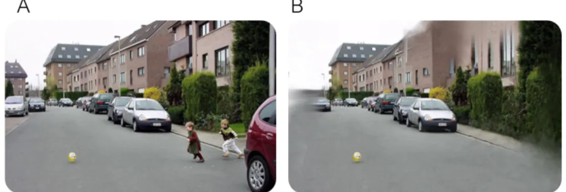
Figure 3.3: Healthy versus glaucomatous vision. (A) Subject view with normal vision. (B)Subject view with glaucoma. Adapted from [41].
As previously mentioned, RGCs neurodegeneration2 plays a key role in glaucoma pathogenesis as it progressively leads to visual field damage. Therefore, glaucoma is traditionally considered an eye disease. Mounting evidence over the last decade, how-ever, suggest that abnormalities in glaucoma spread along the entire length of the visual pathway, rather than limiting their effects to RGCs [3–5, 42–44]. This opens the discus-sion on whether glaucoma pathogenesis should be extended to brain level. A number of neuroimaging studies have been reporting brain changes in glaucomatous patients, from structure - changes in both the grey and white matter (e.g. increase or decrease) -, to connectivity and to functional responses [42, 45–47]. Yet the mechanisms underlying these changes have been extensively debated. The main question relies on the timing, i.e., whether brain changes precede or follow the eye disease.
The most parsimonious explanation seems to be that brain involvement in glaucoma is a consequence of pre-geniculate (i.e., retina and ON) damage propagation through anterograde transsynaptic degeneration3[43, 48]. Nevertheless, the occurrence of retro-grade transsynaptic degeneration4have also been demonstrated, for instance, by changes found in nonvisual loci (e.g., corpus callosum and hippocampus) [43, 49] which suggest another explanation for the source of the changes rather than an indirect consequence of the ocular damage and the subsequent loss of visual input. These findings might be indicative of the brain playing a part as an independent component in glaucoma.
2Progressive loss of neural structure and function that ultimately results in cell death. Neurodegenerative
diseases comprehend a heterogeneous group as each of them exhibits a characteristic profire of regional cell death. Also called transsynaptic degeneration.
3Neurodegeneration caused by loss of input. It occurs “downstream”, that means an injured presynaptic
neuron causes damage to a postsynaptic neuron (e.g. distal axon terminal).
4Neurodegeneration occurring “upstream”. Injury at axonal level spreads back towards the proximal
C
h
a
p
t
e
r
4
Vi s ua l F i e l d D e f e c t s a n d T h e B r a i n
When visual field defects occur in both eyes, due to the retinotopic organization of the visual cortex, a certain part of the brain no longer receives stimulation. How that section of the brain further behaves is highly controversial. One might expect the silencing of the cortical area. However, functional reorganization, as a manifestation of plasticity, has been pointed out as a possible consequence for the absence of visual input.
4.1
Brain Plasticity
Brain plasticity, or neuroplasticity, refers to the ability of the nervous system to adapt its neuronal circuitry in response to environmental changes [50]. Despite the fact that neuroplasticity is thought to be greatest during the early stages of development (child-hood), it seems to be retained throughout a lifespan, even if in a smaller degree [50, 51]. Neuroplasticity has been studied in the past decades, counting on studies in a variety of mammalian species, including humans.
The changes in neuronal architecture yielded by plasticity can be seen at different scales, ranging from synaptic activity and neuronal pathways -synaptic plasticity - as a
result of learning, to cortical maps topography in response to bodily injury, often referred to ascortical remapping [52]. The scope of this thesis only covers the latter.
Deactivation or altered pattern of activation triggers the brain to adapt to the new condition. In the visual system, a visual defect associated to optic nerve damage causes brain deafferentation from the retina. This is usually followed by neurodegeneration. However, when sufficient input from neighbouring sources is still available, visual neu-rons are capable of acquiring new RFs by establishing new connections or by modifying the effectiveness of existing ones, leading to reorganization of the cortical representations, the basis for cortical remapping. For instance, it is widely hypothesized that after retinal
damage, neurons within V1 lesion projection zone (LPZ) (i.e., visual lesion or scotoma transformed into cortical coordinates) can still be stimulated by shifting their RFs from the blind toward intact portions of the visual field [53–55]. This ‘ectopic’ RFs will change V1’s map. Recalling the retinotopic organization of the visual maps, as nearby neurons have RFs at nearby locations in the visual field when neurons shift their RF, the retino-topic map will change accordingly. Moreover, remapping hypothesis is also supported by the increase of RFs’ size which enables the RFs to reach spared visual field and thus, become responsive to stimuli [11, 56].
Remapping as a plasticity phenomenon has been called into question [11, 57]. It is suggested that the responsiveness of neurons within the LPZ is a result of the unmasking of existing feedback signals from higher cortical areas into V1 rather than remapping.
4.2
Predictive Masking
When the information extracted from the visual scene is incomplete, as an attempt to compensate for gaps in perception, the visual system has the ability to predict and interpolate the missing features that are not made available to the cortex. This means that a set of neurons is activated in such a way that a visual stimulus is perceived as arising from a location in the visual field where there is actually no visual input. But how does this actually happen?
PM, or filling-in, is a heterogeneous phenomenon that takes place in different forms on a daily basis, while one observes the surrounding environment. It not only occurs when objects fall behind the blind-spot (figure 4.1), but also when an object is occluded by another, or when one stares steadily for a long time at an image with missing patches of “texture” [58]. The mechanisms underlying the various forms of PM are still not totally clear. Regarding literature, there are two broad proposed models that aim to explain such perceptual phenomenon. First, the symbolic or cognitive theory states that PM is a passive process, the structures from the visual system simply ignore the lack of information and label the region to be completed with the same visual features as the surround [59]. This mechanism is shortly described as “more of the same” [58]. On the other hand, some studies propose that the phenomenon is not a result of simply ignoring a section within the visual field, instead it relies on active neuronal activity. This second model, termed as “isomorphic model”, assumes that PM is mediated by lateral propagation of neural signals, with the spread of activation across the retinotopic map of the visual cortex from the border to the interior of filled-in surface [60]. PM might be alternatively explained by the occurrence of passive cortical remapping, in a way that the receptive fields from the region corresponding to the scotoma or blind-spot are displaced towards the surrounding region representing the scotoma or blind-spot [54].
Activation of early visual areas (V1-V3) is suggested to be involved in representa-tion of filled-in regions of an image. For instance, previous fMRI experiments [61, 62] showed clear activation of the early visual cortex when subjects were asked to perform
4 . 2 . P R E D I C T I V E M A S K I N G
an attention task that consisted of following a filling-in stimulus presented at different places of the visual field. The same stimulus was presented when attention was not con-trolled. Interestingly, both V1 and V2 showed activation regardless of where the subject attended. These findings are indicative of automatic PM of activity at early stages of cortical processing.
PM occurs not only in normal conditions but also in disease. Comparably to our unawareness of the blind-spot, due to this remarkable phenomenon patients with retinal and cortical damage can remain unconscious of their defects [30].
Figure 4.1: Filling-in at the blind-spot. The absence of photoreceptors at the location where the optic nerve leaves the eye results in a blind area in the retina: the blind-spot. To find the blind-spot in your eye, fixate the gaze on the cross at the centre and cover your left eye. Then slowly move towards the image, still staring at the cross. At a certain distance (about 15 cm) the smaller blue circle on the right will disappear. The image falls now on the blind-spot. At the same time, a large yellow disk is seen. By covering the right eye and the left eye’s gaze fixed on the middle cross, the uniform horizontal grading on the right can be seen even though the middle part of the stripes falls inside the blind spot. This is called perceptual ‘completion’ and is due to the pattern filling-in on the left eye’s blind-spot. Reprinted from [6].
C
h
a
p
t
e
r
5
F u n c t i o n a l M a g n e t i c R e s o n a n c e I m a g i n g
The emergence of fMRI in the early 1990s had a real impact on the scientific world, leading the method to become the current mainstay of neuroimaging in cognitive neu-roscience. Since the first carried fMRI study, the number of papers that mention the technique has grown exponentially [95]. The explosion of interest around fMRI lies on its non-invasive nature of measuring and mapping brain activity done with a very good spatial resolution and relatively good temporal resolution.
5.1
The BOLD Signal
In response to stimuli neurons become active in given areas of the brain. This increase in brain activity elicits a need for oxygen and glucose consumption which is overcompen-sated by an increase in regional cerebral blood flow. The local mismatch between oxygen demand and oxygenated blood flow induces changes in the ratio between oxyhemoglobin (hemoglobin bound to oxygen) and deoxyhemoglobin (hemoglobin without bound oxy-gen). Oxyhemoglobin and deoxyhemoglobin have different magnetic properties, which re-sult in different magnetic resonance (MR) signals (see annex I for information about MRI principles). While oxyhemoglobin behaves as a diamagnetic substance, i.e., exhibits a weak repulsion from a magnetic field, deoxygenated hemoglobin is paramagnetic, which means it causes disruption in the magnetic field. These differences in magnetic suscepti-bility will be reflected in an image, allowing us to distinguish active regions (presumably with high oxygen consumption) from inactive regions of the brain. Areas assigned with high concentration of oxyhemoglobin produce a higher signal compared to the one that emerges from areas with lower oxygen levels [63]. The dependence of the recorded signal from blood oxygenation sets the basis of the technique and is the reason why it is often referred to as blood-oxygen-level-dependent (BOLD) imaging.
The regional BOLD signal that results from presentation to sensory space of a given stimulus follows a stereotypical shape referred to as the hemodynamic response (Figure
5.1). The hemodynamic response can last up to 20 seconds and is characterized by a smallinitial dip, followed by a peak, and lastly a variable post stimulus undershoot. There
is a temporal delay to peak of approximately 5s after stimulus processing represented by an initial dip which results from an increase in deoxyhemoglobin concentration. This is then replaced by the positive dominant peak that constitutes the bulk of the BOLD response. Throughout this stage, blood flow increases to immediate metabolic needs. As result, ratio between oxy- and deoxyhemoglobin rises proportionally to the underlying neuronal activity, leading to an increase of the MR signal. If the neuronal activity is extended over time, the peak may extend to a plateau. After stimulus cessation, since the needs of neuronal activity are met, the MR signal drops, slowly returning to baseline level and, eventually, underpasses it. This is called the undershoot effect and derives from the venous bed capacity that tends to cause a normalization of the regional blood volume faster than the changes in blood flow, leading to relatively high deoxyhemoglobin concentration [64].
Figure 5.1: Illustration of a hemodynamic response evoked by neuronal activity in re-sponse to a hypothetical brief stimulus (red bar).The hemodynamic response follows a stereotypical shape that consists of initial dip, positive response (peak), and poststimulus undershoot. Adapted from [64].
The interpretation of the BOLD response is still a topic of active research because it can not be seen as a reflection of neuronal activity. Instead, it must be considered as an indirect measure of neuronal activity through the changes in local oxygenated blood ratios [63].
The hemodynamic response is often treated as a linear time-invariant (LTI) system [65, 66]. Linearity means that the neural response and the BOLD response are scaled by
5 . 1 . T H E B O L D S I G N A L
the same factor. The meaning of linearity is also associated to additivity which means that if there is knowledge what the response is for two separate events, and they both occur close in time, the resulting signal would be the sum of the independent signals. Time invariant means that if an event is shifted byt seconds, the BOLD response is expected
C
h
a
p
t
e
r
6
Vi s ua l F i e l d M a p p i n g
In the field of visual neuroscience, fMRI combined with computational methodologies has been used to respond to the need to identify information that goes beyond detecting the presence or absence of a fMRI signal [67]. The existing techniques take advantage of the retinotopic organization of visual input to measure visual field maps regarding the two orthogonal dimensions needed to identify a specific location in visual space: eccentricity and polar angle (section 2.3.2).
One of the most powerful fMRI techniques to map the visual field is the traveling wave retinotopy (TWR) (also called phase-encoded mapping), illustrated in figure 6.1 [68]. Since its urge in the mid 1990s it has been considered the gold standard for visual field mapping. The TWR allows the estimation of the location in the visual field that maximally excite each fMRI voxel. This is done by using two types of periodic stimuli, expanding/contracting rings and (counter-)clockwise rotating wedges, designed to map each voxel’s prefered eccentricity and polar angle respectively. These stimuli are typically comprised to a set of high-contrast flickering checkerboard patterns which are known from literature to evoke robust neuronal response within V1 of humans [68] and to elicit a BOLD signal modulation on the order of 1%-3% [69]. The name of the technique comes from a resulting traveling wave of cortical activity upon stimulation that travels from one side of the visual field map to the other along iso-angle or iso-eccentricity lines. As a result, the peak modulation alternates periodically across the cortical surface and, thus, the delay can be measured by the phase of the underlying neuronal activity. This phase indicates the most effective stimulus eccentricity and polar angle to fire neurons comprised in that region of the cortex.
Regardless of the potential of TWR to uncover visual field maps in the human brain (approximately sixteen maps have been identified thus far), because of the method’s reliance on the periodicity of the stimulation sequence, it is only suitable for activating
Figure 6.1: Traveling Wave Retinotopy. Traveling wave stimuli typically consist of a set of high contrast checkerboard patterns that move smoothly and periodically across the visual field through a range of eccentricities (expanding/contracting ring) (A) or polar angles (clockwise rotating wedge) (B). The time, or phase, of the peak modulation smoothly varies across the cortical surface (C). In this example six stimulus repetitions are represented. An expanded view of the cortical surface near the calcarine sulcus is overlaid with a color map representing the response phase at each location for both eccentricity (D), elicited by the ring stimuli, and polar angle (E), derived by the wedge in the stimuli sequence. Adapted from [27].
retinotopically-organized areas (early visual cortex). Hence, TWR has limitations when measuring higher order visual field maps with large RFs [27]. Once these limitations became clear, Dumoulin and Wandell decided to improve visual field mapping techniques by developing a model-based approach that extends the notion of RF [17]. As each typical fMRI voxel (3 mm isotropic) cluster the responses of about 3 million neurons and each neuron responds to a preferred location on visual field (RF), based on visual field maps retinotopic organization the RFs within one voxel are expected to present similar characteristics. Therefore, the ensemble of the RFs of all neurons also create a RF, the “population receptive field” (pRF). Unlike TWR approach, the new method provides an estimate of the location and size of the neuronal pRF. Additionally, the pRF approach does not require distinct phase-encoded stimuli, the standard ring and wedge, to infer eccentricity and polar angle. Instead, the orthogonal dimensions can be measured by using a single non-periodic stimuli, a drifting bar (Figure 6.2), cutting down the total number of scans per subject. The underlying goal of this methodology is to test which of a wide range of pRF models best predicts the BOLD signal for each voxel (Figure 6.2). The pRF is modeled as a simple two-dimensional Gaussian defined by three parameters:
x0, y0, and, σ . The two spatial coordinates (x0, y0) assign the pRF center position in the visual field whereas the Gaussian standard deviation (σ ) refers to the pRF size. The latter parameter is of great relevance in the context of visual cortical plasticity, as will be
discussed in more detail further in this thesis. For each voxel, after an extensive database of pRF parameters candidates is created, the method calculates a predicted BOLD signal as result of the overlap between the stimulus information at each time point and the model pRF. The outcome is then convolved with a hemodynamic response function (HRF), to account for the delay in hemodynamic response. Following this, the goodness of fit of the model to explain the actual BOLD response is estimated according to each voxel’s activity over time. This is done until the pRF parameters that best minimize the difference between the prediction and the measured data are found.
Figure 6.2: The population receptive field (pRF) modeling pipeline. Voxel wise the method models the pRF as a two-dimensional Gaussian described by position in visual field (x0,y0) and size (σ of the Gaussian). By overlapping the pRF model with the stimulus aperture (moving bar), a voxel’s activation response is predicted. Then, the predicted BOLD signal is estimated as a result of the convolution between the pRF activation re-sponse with a hemodynamic rere-sponse function (HRF), to account with the hemodynamic response delay. Ultimately, by determining the error between the prediction and the actual measured data, the best fitting model for each cortical location can be estimated. Adapted from [17].
C
h
a
p
t
e
r
7
Po p u l a t i o n R e c e p t i v e F i e l d ( p R F ) C h a n g e s
i n O p t h a l m i c a n d Ne u r o l o g i c D i s e a s e s :
S ta t e - o f -t h e -A rt
Over the last two decades, visual field mapping has been extensively used to infer neu-ronal reorganization resulting from visual field defects or neuro-ophthalmologic diseases. Because of its focus on the analysis of individual participants and the relative amount of detail provided, the pRF model seems ideal to study questions on neuroplasticity – at least in theory. In developmental disorders, studies have consistently reported marked changes that far exceed those observed in health. However, in the adult brain, there is a long-lasting controversy surrounding observations that pRFs can change. The question is whether altered pRF parameters are a reflection of cortical reorganization or whether such changes may be explained by the same dynamics present in the neural circuitry of healthy individuals.
A long tradition of invasive animal neurophysiological studies that aimed to eluci-date how RFs and cortical visual organization are altered lodged arguments that are important for how pRF changes may follow disorder-induced retinal lesions. Through experimentally induced damage to the retina of adult mammals, Gilbert and Wiesel re-ported remarkable changes in V1 RFs [9]. Namely, neurons with RFs near the edge of the lesion increased the RF size whereas neurons with RFs inside the insult reconfigured their position towards portions of spared retina. The authors claimed the findings as a result of reorganization of the RFs properties due to synaptic changes intrinsic to the cortex. However, this conclusion was contended by others [57] who argued that changes in RF properties do not require to be explained by cortical reorganization. Alternatively, the presence of activity in deprived visual cortex reported previously may be the result of gain adjustments that reduce feedforward information or a downregulation of inhibition.
In human studies, stimulus manipulations to mimic blind regions – e.g. by removing the stimulus at a given position [11, 70] or by diminishing light to simulate scotopic vision [71] (when only rods operate) - have been a powerful tool to investigate the effects of such visual deficits in pRF measurements. Reduced signal amplitudes, shifted pRFs and scaled pRF sizes in the vicinity of the simulated lesion site have been often observed as a result of these simulations. As so, the differences in pRF properties arising from simulation of lesions in healthy adults support and extend the notion that changes in neuronal populations are not unique identifiers of cortical reorganization.
In healthy adults, the resulting retinotopic maps are stable over time [72]. Hence, it would appear that changes in maps or population properties should be a good indication for the presence of neuroplasticity. In a study conducted by Baseler and collaborators in individuals diagnosed with macular degeneration (MD) - an ocular disease characterized by a visual blind spot (scotoma) in central vision - pRF properties were measured in the foveal region of the patients [11]. It was found that the pRFs of voxels representing both the scotomatic area and neighboring regions are displaced and changed in size. However, well-sighted controls in whom a central scotoma was simulated shared the same pattern of results. This finding challenged the notion of electrophysiological studies that changes in RFs are evidence of cortical reorganization. Hence, the authors argued for a lack of neuroplasticity in patients with MD. Barton and Brewer also found comparable shifts in pRF position and scaling of pRF size in their experiment that used scotopic illumination levels to examine the "rod scotoma"in the central visual field [71]. Others further confirmed the observation of altered pRFs in healthy individuals in the vicinity of a simulated scotoma [73, 74]. This implies that observed differences in pRF properties in patients relative to controls may simply reflect normal responses to a lack in visual input rather than a reorganization of the visual cortex.
In the case of congenital visual pathway abnormalities that affect the optic nerve cross-ing at the chiasm, e.g. achiasm, albinism and hemi-hydranencephaly, each hemisphere receives input from the ipsi- and contralateral visual hemifield. In other words, each hemisphere grossly represents both left and right visual hemifields. Accordingly, several studies revealed overlapping visual fields and bilateral vertical symmetric pRF repre-sentations [75–77]. Such evidences surpass the realm of typical cortical reorganization. Nevertheless, no changes in pRF sizes and other properties of visual pathways have been found, thus it is speculated that visual functions is preserved in these pathologies by reorganization of intracortical connections rather than by large-scale reorganization of the visual cortex.
Given that visual neuroplasticity is greatest during early stages of development (child-hood), the characterization of the pRF properties has special relevance to test, in vivo, the presence of atypical properties of the visual cortex during development and plasticity. Changes in pRF size have been reported in a series of studies on developmental disorders, such as amblyopia, commonly referred to as the lazy eye, characterized by a reduction in
![Figure 2.1: Schematic anatomy of the eye. Reprinted from [21].](https://thumb-eu.123doks.com/thumbv2/123dok_br/19187241.948155/32.892.272.607.246.564/figure-schematic-anatomy-eye-reprinted.webp)
![Figure 3.2: Ocular damage in primary POAG and PACG. Reprinted from [39].](https://thumb-eu.123doks.com/thumbv2/123dok_br/19187241.948155/41.892.161.726.143.540/figure-ocular-damage-primary-poag-pacg-reprinted.webp)