An implementation of flexible RBF neural networks

U

NIVERSIDADE DE

L

ISBOA

Faculdade de Ciˆencias

Departamento de Inform´atica

AN IMPLEMENTATION OF

FLEXIBLE RBF NEURAL NETWORKS

Fernando Manuel Pires Martins

MESTRADO EM INFORM ´

ATICA

U

NIVERSIDADE DE

L

ISBOA

Faculdade de Ciˆencias

Departamento de Inform´atica

AN IMPLEMENTATION OF

FLEXIBLE RBF NEURAL NETWORKS

Fernando Manuel Pires Martins

DISSERTAC

¸ ˜

AO

Projecto orientado pelo Prof. Doutor Andr´e Os´orio Falc˜ao

MESTRADO EM INFORM ´

ATICA

Acknowledgements

I wish to acknowledge those who, either by change or simple misfortune, were involved in my MSc.

I start by acknowledging Professor Andr´e Falc˜ao for the trust, the guidance and the pa-tience shown for the long months this work took, never giving up on me, even when the bad times seemed to put an early end to my MSc.

I wish to acknowledge my good friend Paulo Carreira, who has been an inspiration and who has always supported and pushed me into the final goal of writing this dissertation. A special thanks goes for my family. There are no words to express my gratitude nor to express how fantastic they were in supporting me. Without their support, this disserta-tion would certainly not exist.

I wish to thanks to my parents Julia and Fernando, for the support and education that al-lowed me to come this far, and to my grandmother Maria Teresa, for her inspiring reading and writting passion.

Finally, I have an endless debt to my beloved wife Vilma, which is responsible for, almost magically, getting me the time to work on my MSc. I also have a time debt to my daugh-ters, Sofia and Camila, for the countless times that I had to refuse to play with in this last four years.

Resumo

Sempre que o trabalho de investigac¸˜ao resulta numa nova descoberta, a comunidade ci-ent´ıfica, e o mundo em geral, enriquece. Mas a descoberta cient´ıfica per se n˜ao ´e sufici-ente. Para beneficio de todos, ´e necess´ario tornar estas inovac¸˜oes acess´ıveis atrav´es da sua f´acil utilizac¸˜ao e permitindo a sua melhoria, potenciando assim o progresso cient´ıfico.

Uma nova abordagem na modelac¸˜ao de n´ucleos em redes neuronais com Func¸˜oes de Base Radial (RBF) foi proposta por Falc˜ao et al. em Flexible Kernels for RBF Networks [14]. Esta abordagem define um algoritmo de aprendizagem para classificac¸˜ao, inovador na ´area da aprendizagem das redes neuronais RBF. Os testes efectuados mostraram que os resultados est˜ao ao n´ıvel dos melhores nesta ´area, tornando como um dever ´obvio para com a comunidade cient´ıfica a sua disponibilizac¸˜ao de forma aberta. Neste contexto, a motivac¸˜ao da implementac¸˜ao do algoritmo de n´ucleos flex´ıveis para redes neuronais RBF (FRBF) ganhou novos contornos, resultando num conjunto de objectivos bem definidos: (i) integrac¸˜ao, o FRBF deveria ser integrado, ou integr´avel, numa plataforma facilmente acess´ıvel `a comunidade cient´ıfica; (ii) abertura, o c´odigo fonte deveria ser aberto para potenciar a expans˜ao e melhoria do FRBF; (iii) documentac¸˜ao, imprescind´ıvel para uma f´acil utilizac¸˜ao e compreens˜ao; e (iv) melhorias, melhorar o algoritmo original, no proce-dimento de c´alculo das distˆancias e no suporte de parˆametros de configurac¸˜ao. Foi com estes objectivos em mente que se iniciou o trabalho de implementac¸˜ao do FRBF.

O FRBF segue a tradicional abordagem de redes neuronais RBF, com duas camadas, dos algoritmos de aprendizagem para classificac¸˜ao. A camada escondida, que cont´em os n´ucleos, calcula a distˆancia entre o ponto e uma classe, sendo o ponto atribu´ıdo `a classe com menor distˆancia. Este algoritmo foca-se num m´etodo de ajuste de parˆametros para uma rede de func¸˜oes Gaussianas multi-vari´aveis com formas el´ıpticas, conferindo um grau de flexibilidade extra `a estrutura do n´ucleo. Esta flexibilidade ´e obtida atrav´es da utilizac¸˜ao de func¸˜oes de modificac¸˜ao aplicadas ao procedimento de c´alculo da distˆancia, que ´e essencial na avaliac¸˜ao dos n´ucleos. ´E precisamente nesta flexibilidade e na sua aproximac¸˜ao ao Classificador Bayeseano ´Optimo (BOC), com independˆencia dos n´ucleos em relac¸˜ao `as classes, que reside a invocac¸˜ao deste algoritmo.

O FRBF divide-se em duas fases, aprendizagem e classificac¸˜ao, sendo ambas seme-lhantes em relac¸˜ao `as tradicionais redes neuronais RBF. A aprendizagem faz-se em dois passos distintos. No primeiro passo: (i) o n´umero de n´ucleos para cada classe ´e definido

atrav´es da proporc¸˜ao da variˆancia do conjunto de treino associado a cada classe; (ii) o conjunto de treino ´e separado de acordo com cada classe e os centros dos n´ucleos s˜ao de-terminados atrav´es do algoritmo K-Means; e (iii) ´e efectuada uma decomposic¸˜ao espectral para as matrizes de covariˆancia para cada n´ucleo, determinando assim a matriz de vecto-res pr´oprios e os valovecto-res pr´oprios corvecto-respondentes. No segundo passo s˜ao encontrados os valores dos parˆametros de ajuste de expans˜ao para cada n´ucleo. Ap´os a conclus˜ao da fase de aprendizagem, obt´em-se uma rede neuronal que representa um modelo de classificac¸˜ao para dados do mesmo dom´ınio do conjunto de treino. A classificac¸˜ao ´e bastante simples, bastando aplicar o modelo aos pontos a classificar, obtendo-se o valor da probabilidade do ponto pertencer a uma determinada classe. As melhorias introduzidas ao algoritmo original, definidas ap´os an´alise do prot´otipo, centram-se: (i) na parametrizac¸˜ao, permi-tindo a especificac¸˜ao de mais parˆametros, como por exemplo o algoritmo a utilizar pelo K-Means; (ii) no teste dos valores dos parˆametros de ajuste de expans˜ao dos n´ucleos, testando sempre as variac¸˜oes acima e abaixo; (iii) na indicac¸˜ao de utilizac¸˜ao, ou n˜ao, da escala na PCA; e (iv) na possibilidade do c´alculo da distˆancia ser feito ao centr´oide ou `a classe.

A an´alise `a plataforma para desenvolvimento do FRBF, e das suas melhorias, resultou na escolha do R. O R ´e, ao mesmo tempo, uma linguagem de programac¸˜ao, uma plata-forma de desenvolvimento e um ambiente. O R foi seleccionado por v´arias raz˜oes, de onde se destacam: (i) abertura e expansibilidade, permitindo a sua utilizac¸˜ao e expans˜ao por qualquer pessoa; (ii) reposit´orio CRAN, que permite a distribuic¸˜ao de pacotes de ex-pans˜ao; e (iii) largamente usado para desenvolvimento de aplicac¸˜oes estat´ısticas e an´alise de dados, sendo mesmo o standard de facto na comunidade cient´ıfica estat´ıstica.

Uma vez escolhida a plataforma, iniciou-se a implementac¸˜ao do FRBF e das suas me-lhorias. Um dos primeiros desafios a ultrapassar foi a inexistˆencia de documentac¸˜ao para desenvolvimento. Tal facto implicou a definic¸˜ao de boas pr´aticas e padr˜oes de desenvolvi-mento espec´ıficos, tais como documentac¸˜ao e definic¸˜ao de vari´aveis. O desenvolvidesenvolvi-mento do FRBF dividiu-se em duas func¸˜oes principais, frbf que efectua o procedimento de aprendizagem e retorna o modelo, e predict uma func¸˜ao base do R que foi redefi-nida para suportar o modelo gerado e que ´e respons´avel pela classificac¸˜ao. As primeiras vers˜oes do FRBF tinham uma velocidade de execuc¸˜ao lenta, mas tal n˜ao foi inicialmente considerado preocupante. No entanto, alguns testes ao procedimento de aprendizagem eram demasiado morosos, passando a velocidade de execuc¸˜ao a ser um problema cr´ıtico. Para o resolver, foi efectuada uma an´alise para identificar os pontos de lentid˜ao. Esta acc¸˜ao revelou que os procedimentos de manipulac¸˜ao de objectos eram bastante lentos. Assim, aprofundou-se o conhecimento das func¸˜oes e operadores do R que permitissem efectuar essa manipulac¸˜ao de forma mais eficiente e r´apida. A aplicac¸˜ao desta acc¸˜ao cor-rectiva resultou numa reduc¸˜ao dr´astica no tempo de execuc¸˜ao. O processo de qualidade do FRBF passou por trˆes tipos de testes: (i) unit´arios, verificando as func¸˜oes

mente; (ii) de caixa negra, testando as func¸˜oes de aprendizagem e classificac¸˜ao; e (iii) de precis˜ao, aferindo a qualidade dos resultados. Considerando a complexidade do FRBF e o n´umero de configurac¸˜oes poss´ıveis, os resultados obtidos foram bastante satisfat´orios, mostrando uma implementac¸˜ao s´olida. A precis˜ao foi alvo de atenc¸˜ao especial, sendo pre-cisamente aqui onde n˜ao foi plena a satisfac¸˜ao com os resultados obtidos. Tal facto adv´em das discrepˆancias obtidas entre os resultados do FRBF e do prot´otipo, onde comparac¸˜ao dos resultados beneficiou sempre este ´ultimo. Uma an´alise cuidada a esta situac¸˜ao reve-lou que a divergˆencia acontecia na PCA, que ´e efectuada de forma distinta. O pr´oprio R possui formas distintas de obter os vectores pr´oprios e os valores pr´oprios, tendo essas formas sido testadas, mas nenhuma delas suplantou os resultados do prot´otipo.

Uma vez certificado o algoritmo, este foi empacotado e submetido ao CRAN. Este processo implicou a escrita da documentac¸˜ao do pacote, das func¸˜oes e classes envolvidas. O pacote ´e distribu´ıdo sob a licenc¸a LGPL, permitindo uma utilizac¸˜ao bastante livre do FRBF e, espera-se, potenciando a sua explorac¸˜ao e inovac¸˜ao.

O trabalho desenvolvido cumpre plenamente os objectivos inicialmente definidos. O algoritmo original foi melhorado e implementado na plataforma standard usada pela co-munidade cient´ıfica estat´ıstica. A sua disponibilizac¸˜ao atrav´es de um pacote no CRAN sob uma licenc¸a de c´odigo aberto permite a sua explorac¸˜ao e inovac¸˜ao. No entanto, a implementac¸˜ao do FRBF n˜ao se esgota aqui, existindo espac¸o para trabalho futuro na reduc¸˜ao do tempo de execuc¸˜ao e na melhoria dos resultados de classificac¸˜ao.

Keywords: Func¸˜oes de Base Radial, Redes Neuronais, N´ucleos Flex´ıveis, R

Abstract

This dissertation is focused on the implementation and improvements of the Flexible

Ra-dial Basis Function Neural Networks algorithm. It is a clustering algorithm that describes

a method for adjusting parameters for a Radial Basis Function neural network of multi-variate Gaussians with ellipsoid shapes. This provides an extra degree of flexibility to the kernel structure through the usage of modifier functions applied to the distance computa-tion procedure.

The focus of this work is the improvement and implementation of this clustering al-gorithm under an open source licensing on a data analysis platform. Hence, the alal-gorithm was implemented under the R platform, the de facto open standard framework among statisticians, allowing the scientific community to use it and, hopefully, improve it. The implementation presented several challenges at various levels, such as inexistent develop-ment standards, the distributable package creation and the profiling and tuning process. The enhancements introduced provide a slightly different learning process and extra con-figuration options to the end user, resulting in more tuning possibilities to be tried and tested during the learning phase. The tests performed show a robust implementation of the algorithm and its enhancements on the R platform.

The resulting work has been made available as a R package under an open source licensing, allowing everyone to used it and improve it. This contribution to the scientific community complies with the goals defined for this work.

Keywords: Radial Basis Function, Neural Network, Flexible Kernels, R

Contents

Figure List xvii

Table List xix

Algorithm List xxi

1 Introduction 1

1.1 Motivation. . . 2

1.2 Goals . . . 2

1.3 Contribution . . . 3

2 Flexible Kernels for RBF Networks 5 2.1 Radial Basis Functions . . . 5

2.2 Radial Basis Functions Neural Networks . . . 6

2.2.1 Neural Architecture. . . 7

2.2.2 Radial Basis Function Network Training. . . 8

2.2.3 Classification with Radial Basis Function Network . . . 10

2.3 Flexible Kernels for RBF Neural Networks . . . 10

2.3.1 Flexible Kernels . . . 11

2.4 Proof of Concept Prototype . . . 16

2.5 Improvements . . . 18

3 R 21 3.1 What is R?. . . 21

3.2 R Language . . . 22

3.3 R Workspace . . . 23

3.4 Comprehensive R Archive Network . . . 23

3.5 R Development . . . 24

3.5.1 Objects . . . 24

3.5.2 Function Overloading . . . 24

3.5.3 Application Programming Interface . . . 25

3.5.4 Debug . . . 25 xiii

3.5.5 Why R? . . . 25

4 FRBF Implementation 27 4.1 Development Environment . . . 27

4.1.1 R Development Environment. . . 28

4.1.2 Documentation Development Environment . . . 28

4.1.3 Packaging Development Environment . . . 28

4.2 Implementation . . . 29

4.2.1 Development . . . 29

4.2.2 Functions and Operators Used . . . 31

4.2.3 Model . . . 33 4.2.4 Print. . . 34 4.2.5 Learning . . . 35 4.2.6 Prediction . . . 35 4.2.7 Tuning . . . 36 4.2.8 Problems Found . . . 37 4.3 Tests . . . 38

4.3.1 Execution Behaviors Observed . . . 38

4.3.2 Results . . . 40 4.4 User Interface . . . 42 4.4.1 FRBF . . . 42 4.4.2 Predict . . . 44 4.4.3 Usage . . . 44 4.5 R Packaging . . . 45 4.5.1 Package Structure. . . 46 4.5.2 Help Files . . . 47 4.5.3 Distribution File . . . 47 4.5.4 Problems Found . . . 48

4.5.5 Installing and Uninstalling . . . 48

5 Conclusions 51 5.1 Work Performed. . . 51

5.2 Release . . . 52

5.3 Future Work . . . 52

A Static Definitions 53 A.1 Constant Definition . . . 53

A.2 Class Definition . . . 54 xiv

B FRBF Code Sample 57 B.1 Find S . . . 57 B.2 FRBF . . . 61 B.3 Get PCA . . . 63 B.4 Predict . . . 64 C Tests 65 D Documentation 69 E Packaging 71 E.1 R Packaging Script . . . 71

E.2 Shell Packaging Script . . . 72

Abbreviations 75

Bibliography 79

Index 80

List of Figures

2.1 A RBF neural network from Mitchell [36]. . . 7

2.2 A RBF neural network with NN terminology adapted from Mitchell [36]. 8 2.3 An example of a spiky and a broad Gaussian, adapted from Wikipedia [57]. 9 2.4 A RBF neural network classification example adapted from Mitchell [36]. 10 2.5 Example of shapes. . . 12

2.6 A FRBF classification example adapted from Mitchell [36]. . . 16

2.7 Prototype usage example. . . 18

3.1 Function overloading definition. . . 25

4.1 An example of code declaration and documentation.. . . 30

4.2 An example of the operators usage.. . . 33

4.3 Remora predict function overloading. . . 36

4.4 Black box test script execution example. . . 39

4.5 A FRBF cluster grab making a broad Gaussian example. . . 40

4.6 Example of the FRBF functions usage. . . 46

List of Tables

2.1 Distance weighting function models from Falc˜ao et al. [14]. . . . 13

2.2 StatLog results using the prototype, adapted from Falc˜ao et al. [14]. . . . 17

4.1 FRBF testing data sets. . . 38

4.2 FRBF and prototype accuracy comparison results. . . 41

4.3 FRBF training and testing accuracy results. . . 41

4.4 weighting functionparameter values, following Falc˜ao et al. [14]. 44

4.5 Acceptable values forverboseparameter. . . 44

List of Algorithms

2.1 Stage One of Flexible Kernels Learning Procedure . . . 14

2.2 Stage Two of Flexible Kernels Learning Procedure . . . 15

4.1 Overview of thefrbffunction steps . . . 35

Chapter 1

Introduction

Whenever scientific work results in a new discovery, the scientific community, and the world in general, becomes richer. But the scientific discovery by itself is not sufficient, it must be accessible and easily usable by everyone, so that people take advantage of such innovations. Making the scientific breakthroughs accessible to everyone is therefor a major contribution to the scientific community since it provides a way to everyone use it, test it and, ultimately, improve it.

An approach for modeling kernels in Radial Basis Function (RBF) networks has been proposed in Flexible Kernels for RBF Networks [14] by Falc˜ao et al.. This approach focus on a method for adjusting parameters for a network of multivariate Gaussians with ellip-soid shapes and provides extra degree of flexibility to the kernel structure. This flexibility is achieved through the usage of modifier functions applied to the distance computation procedure, essential for all kernel evaluations.

This new algorithm was an innovation within the neural networks learning area based on RBF neural networks. A concept proof implementation of this architecture has proved capable of solving difficult classification problems with good results in real life situations. This was a stand alone implementation with the specific goal to prove the concept and, therefor was available only to the research team members. Consequently, making this work accessible to everyone was the next logical step for this new algorithm.

In this context, an implementation of the Flexible kernels for RBF neural network (FRBF) algorithm under a widely spread scientific platform arise. A widely used platform by the scientific community should be targeted, hence the R platform has been chosen, since it is the open source de facto standard statistical platform. The resulting implemen-tation was also packed and distributed under open source licensing, allowing anyone to modify it and, eventually, improve it. Some enhancements were performed on the original algorithm, some focused on the algorithm parameterization and others on the algorithm itself. The usage of the available base R functions that were, themselves, already param-eterized helped on this task and, as a result, a high number of possible configurations to the end user was delivered.

Chapter 1. Introduction 2

This dissertation is organized as follows: Chapter1introduces this dissertation, Chap-ter2describes the Radial Basis Function neural networks, details the flexible kernels clus-tering algorithm, which is the genesis of this work, and the improvements performed to it. The implementation framework R is covered in the Chapter3and the implementation of the new algorithm is detailed in Chapter4. Finally, Chapter5concludes this dissertation and resumes the goals achieved.

1.1

Motivation

Having obtained such good results with the FRBF tests, it was obvious that it should be made available to everyone. Hence, the main stimulus behind this work was to provide an easy way for the scientific community to use FRBF.

The proof of concept implementation was developed as a stand alone application, so it was a very specific computer program that served a single purpose and was not ready, nor meant, to be used in any other way. Hence, it did not served the purpose of distribution nor integration with frameworks, or other applications, making it a non eligible solution.

There was also a second motivation for this work, focused on the enhancement of the algorithm. It early became clear that the original algorithm could be improved and a new implementation was the perfect scenario for such task, since it provided the chance to perform the enhancements.

Hence, the need of a new FRBF implementation emerged. The motivation of this work was to (i) provide an easy to use implementation to the scientific community, (ii) integrate with, or within, a framework, (iii) improve the original algorithm and (iv) be open to receive improvements from others.

1.2

Goals

The motivation resulted in the set of specific goals. The main goal of this work was to deliver a new, open and integrated, implementation of the FRBF and a second goal was to improve the original algorithm.

These goals have been established after the identification of (i) the need of an FRBF implementation that would be integrated with, or within, a framework and (ii) the oppor-tunity of enhance the original algorithm with some improvements. In detail, the goals for this work have been set as:

Integration. The implementation of FRBF only made sense if it could be integrated with, or within, a framework or a third party application. The selected platform was R since R is the de facto open standard among statisticians. R is also an integrated suite of software facilities for statistical computing, data manipulation, calculation

Chapter 1. Introduction 3

and graphical display. All this makes R a perfect target for this new FRBF imple-mentation. Delivering the FRBF implementation as a R expansion package com-plies with this goal.

Open source. In order to allow others to expand and improve FRBF the source code had to be made open for the public. Thus, the resulting implementation was delivered under an open source licensing, allowing anyone to access the source code, explore it and even improve it.

Documentation. The implementation process followed the usual software development good practices. This means, among other things, that everything is documented. The entire source code is documented, the distributed R package is documented and the improvements are also documented. Since there are several distinct docu-mentation levels involved here, the docudocu-mentation itself comes in different formats but is, in general, easily accessible. This provides an easy way to the understanding of the FRBF implementation to anyone willing to go deeper in the subject.

Enhancements. The enhancements of the original algorithm were defined as improve-ments to the distance calculation procedure and the support for more configuration options. The new implementation also had to support the original algorithm spec-ification, meaning disabling the improvements, a feature that also comes up as a configuration option. In practice, this means that the end user has more power and flexibility to configure the algorithm when searching for the best classification model for a given domain.

The goals stated above fully respond to the initial motivation identified on the prece-dent section. The achieve of these goals resulted in an easy way to the scientific commu-nity to use FRBF on a well known and standard platform.

1.3

Contribution

Regarding the previously stated goals in the previous section, the main contribution of this work is the deliver of an improved FRBF implementation to the scientific community.

The enhancements performed over the original algorithm are a small contribution to the RBF neural network learning algorithms. The improvements included in this imple-mentation provide the end user more power and flexibility when parameterizing the learn-ing task. This results in a much wide number of possibilities available when searchlearn-ing for the best classification model for a given problem.

The implementation of the FRBF as a R expansion package is, by itself, a contribu-tion to the de facto standard statistical platform used by the scientific community. The packaging of the algorithm provides a standard way to distribute, use and document the

Chapter 1. Introduction 4

FRBF algorithm on this widely used platform. Finally, the usage of an open source li-censing model allows anyone to explore and extend it to their own needs, opening a way for future improvements and an yet better implementation or classification algorithm.

Chapter 2

Flexible Kernels for RBF Networks

This chapter describes the Radial Basis Functions (RBF) briefly, explains the RBF neu-ral networks, details the Flexible RBF neuneu-ral networks algorithm and the correspondent enhancements introduced to the original version.

The Flexible Kernels for RBF neural networks algorithm, defined by Falc˜ao et al. in [14], was a breakthrough in the RBF neural networks. It is a learning algorithm used for classification that provides adjustment of parameters, allowing extra flexibility to the kernel structure. The tests performed proved that this algorithm is effective with real life data.

2.1

Radial Basis Functions

A Radial Basis Function is a function whose value depends on the distance from a point

𝑥 to a center point 𝑐, so that

𝜙(x, c) = 𝜙(∥x − c∥) (2.1)

The norm is to use the Euclidean distance, but other distance functions can be used. RBF neural networks are typically used to build up function approximations. This means that a RBF neural network is used as a function that closely matches, or approxi-mates, or describes, a target function on a specific domain. The target function itself may actually be unknown. But, in such cases, there is usually enough data from the target func-tion domain from which one can learn, and use that knowledge to define an approximate function.

The sum of the RBF is commonly used to approximate given functions. This can be interpreted as a rather simple one layer type of artificial neural network (NN) that can be expressed by the equation

𝑔(𝑥) = 𝑁 ∑ 𝑢=1 𝑤𝑢𝜙(∣∣𝑥 − 𝑐𝑢∣∣) (2.2) 5

Chapter 2. Flexible Kernels for RBF Networks 6

where the approximating function𝑔(𝑥) is represented as a sum of 𝑁 radial basis

func-tions, each associated with a different center𝑐𝑢, and weighted by an appropriate coeffi-cient𝑤𝑢. The 𝑤𝑢 coefficient is a weight that can be estimated using any of the standard iterative methods for neural networks, like the least squares function. In this case, the Ra-dial Basis Functions are the activation functions of the neural network. RBF are covered in detail by Hastie et al. in [23] and by Buhmann in [6].

2.2

Radial Basis Functions Neural Networks

RBF neural network, as introduced in the prior section, is a type of artificial neural net-work constructed from a function distance. The function distance is obtained from the known domain data, called training data, which means the RBF neural network is a learn-ing method that will try to find patterns in the trainlearn-ing data and model it as a network. In particular, the distance function is used to determine the weight of each known data point, the training example, and it is called Kernel function. The work of Yee et al. in [59] and Hastie et al. in [23] cover RBF neural networks in detail.

Learning with RBF neural networks is therefor an approach to function approxima-tion, which is closely related to distance weighted regression and to artificial neural net-works. The term regression is widely used by the statistical learning community to refer the problem of approximating real valued functions, while weighted distance refers to the contribution that each training example has, by calculating the weight of its distance to a center point. This subject is widely studied by the scientific community, some examples are [41,5,22,4,36,24,35,23,59,58]. In particular, Park et al. in [40] studies universal approximation using RBF neural networks.

As specified in detail by Mitchell in [36], in the RBF neural network approach the learned hypothesis is a function of the form

ˆ 𝑓 (𝑥) = 𝑤0+ 𝑘 ∑ 𝑢=1 𝑤𝑢𝐾𝑢(𝑑(𝑥𝑢, 𝑥)) (2.3)

where𝑘 is a parameter provided by the user that specifies the number of kernel functions

to be included,𝑥 is the point being classified, each 𝑥𝑢is an instance from𝑋, the training data, and𝐾𝑢(𝑑(𝑥𝑢, 𝑥)) is the kernel function, that depends on a distance function.

It is easy to understand that the distance function is essential for all kernel evaluations. As previously stated, the kernel function is actually the distance function that is used to determine the weight of each training example. In Equation2.3above, it is defined so that it decreases as the distance𝑑(𝑥𝑢, 𝑥) increases.

Even though ˆ𝑓 (𝑥) is a generic approximation to 𝑓 (𝑥), the function that correctly

clas-sifies each instance, the contribution from each of the kernel terms is located in a region near the𝑥𝑢 point. It is common to choose each kernel function to be a Gaussian function

Chapter 2. Flexible Kernels for RBF Networks 7

centered at the point𝑥𝑢 with some variance𝜎𝑢2, so that

𝐾𝑢(𝑑(𝑥𝑢, 𝑥)) = 𝑒

1 2𝜎2𝑢𝑑

2_{(𝑥𝑢,𝑥)}

(2.4) This equation is the common Gaussian kernel function for RBF neural networks, but other kernel functions can be used. The kernel functions have been widely studied and is easy to find literature about it, for instance, Hastie et al. in [23] describes the Gaussian RBF and Powell in [42] details RBF approximation to polynomial functions.

2.2.1

Neural Architecture

The function in Equation2.3can be viewed as describing a two layer network where the first layer computes the values of the various𝐾𝑢(𝑑(𝑥𝑢, 𝑥)), and the second layer computes a linear combination of the unit values calculated in the first layer. In the basic form, all inputs are connected to each hidden unit. Each hidden unit produces an activation determined by a Gaussian function, or any other function used, centered at some instance

𝑥𝑢. Therefor, its activation will be close to zero unless the input𝑥 is near 𝑥𝑢. The output unit produces a linear combination of the hidden unit activations. An example of a RBF neural network is illustrated in Figure2.1.

Figure 2.1: A RBF neural network from Mitchell [36].

In the neural network terminology, the variables of Equation2.3are called differently, though they mean the same. In particular, 𝑘 is the number of neurons in the hidden

layer, 𝑥𝑢 is the center vector for neuron 𝑢, and 𝑤𝑢 are are weights of the linear output neuron. An example of a RBF neural network with the neural network terminology is illustrated in Figure2.2. The work of Haykin in [24] discusses neural networks in detail while Hartman et al. in [22] focus on neural networks with Gaussian hidden units as universal approximations, and more recently, Zainuddin et al. in [60] discusses function approximation using artificial neural networks.

Chapter 2. Flexible Kernels for RBF Networks 8

Figure 2.2: A RBF neural network with NN terminology adapted from Mitchell [36].

2.2.2

Radial Basis Function Network Training

RBF neural networks are built eagerly from local approximations centered around the training examples, or around clusters of training examples, since all that is known is the set of the training data points. Hence, the training data set is used to build the RBF neural network, which is achieved over two consecutive stages. The first stage selects the centers and set the deviations of the neural network hidden units. The second stage optimizes the linear output layer of the neural network.

First Stage

As previously stated, on the first stage the centers must be selected. The center selection should be assigned to reflect the natural data clustering. The selection can be done uni-formly or non-uniuni-formly. The non-uniform selection is especially suited if the training data points themselves are found to be distributed non-uniformly over the testing data. The most common methods for center selection are:

Sampling: use randomly chosen training points. Since they are randomly selected, they will represent the distribution of the training data in a statistical sense. However, if the number of training data points is not large enough, it may actually be a poor representation of the entire data domain.

K-Means: use the K-Means algorithm, explained by MacQueen and Bishop in [34,4], to select an optimal set of points that are placed at the centroids of clusters of training data. Given a 𝑘 number of clusters, it adjusts the positions of the centers so that

(i) each training point belongs to the nearest cluster center, and (ii) each cluster center is the centroid of the training points that belong to it. The EM algorithm, explained in detail by Dempster et al. in [13], can also be used for this task.

Chapter 2. Flexible Kernels for RBF Networks 9

Once the centers are assigned, it is time to set the deviations. The size of the devi-ation determines how spiky the Gaussian functions are. If the Gaussians are too spiky, the network will not interpolate between known points, and thus loses the ability to gen-eralize. On the other end, if the Gaussians are very broad the network loses fine detail. This is actually a common manifestation of the fitting dilemma, over-fitting is as bad as under-fitting. For an example of such Gaussian shapes, see Figure2.3.

Spiky Gaussian at the left and broad Gaussian on the right.

Figure 2.3: An example of a spiky and a broad Gaussian, adapted from Wikipedia [57]. To obtain a good result, the deviations should typically be chosen so that Gaussians overlap with a few nearby centers. The most common methods used for such task are: Explicit: the deviation is defined by a specific value, for instance a constant.

Isotropic: the deviation is the same for all units and is selected heuristically to reflect the number of centers and the volume of space they occupy.

K-Nearest Neighbor: where each unit deviation value is individually set to the mean distance to its K nearest neighbors. Hence, deviations are smaller in tightly packed areas of space, preserving detail, and higher in sparse areas of space. The work of Cover et al. in [11] and Haykin in [24] give a detailed insight.

Second Stage

Once the centers and deviations have been set, the second stage takes place. In this stage, the output layer can be optimized using a standard linear optimization technique, the Singular Value Decomposition algorithm (SVG) as described by Haykin in [24].

The singular value decomposition is an important way of factoring matrices into a series of linear approximations that expose the underlying structure of the matrix. This allows faster computation since patterns are used instead of the entire data itself.

Chapter 2. Flexible Kernels for RBF Networks 10

The training of the RBF neural network is concluded when this stage finishes. The result is a trained neural network that defines a model for the domain of the training data.

2.2.3

Classification with Radial Basis Function Network

Classification using the learned RBF neural network is quite simple. Once the RBF neural network is defined through the learning procedure, as described in the previous section, it holds a model that can be applied to new, unseen, data of the same domain as the training data. Hwang et al. in [26] describe an efficient method to construct a RBF neural network classifier.

When the model is applied, the artificial neural network will be able to classify, hope-fully correctly, the new data by calculating the distance of each new data point to each of the centers of the model. This is performed through the activation of the hidden units, as in any other artificial neural network. When a new data point𝑥 is being classified, it will

activate the hidden unit𝑥𝑢, where𝑥𝑢is the nearest center to the point𝑥. Following Figure

2.4, the classification of𝑥 results in (i) 20% of probability to belong to the first cluster of

class𝐴, (ii) 10% of probability to belong to the second cluster of class 𝐴, (iii) 40% of

probability to belong to class𝐵, and (iv) 30% of probability to belong to class 𝐶.

Figure 2.4: A RBF neural network classification example adapted from Mitchell [36]. To summarize, when the obtained RBF neural network model is applied to a data point

𝑥 it will return the 𝑥𝑢that is the nearest center to𝑥, and classification happens.

2.3

Flexible Kernels for RBF Neural Networks

The original Flexible Kernels for RBF neural networks algorithm, developed by Falc˜ao et

al. in [14], was a breakthrough in the RBF neural networks area. This learning algorithm is used for classification and distinguishes itself from other RBF neural network algo-rithms by introducing extra flexibility to the kernel and by its approximation to the Bayes

Chapter 2. Flexible Kernels for RBF Networks 11

Optimal Classifier (BOC) with independent kernel regarding the classes. The work is the genesis of this dissertation. It follows the earlier works of Albrecht et al. and Bishop et

al. in [1,4] and will be explained in the next sections.

As described by Hastie et al. in [23], kernel methods achieve flexibility by fitting simple models in a region local to the target point 𝑥𝑢. Localization is achieved via a weighting kernel𝐾𝑢, and individual observations receive weights𝐾𝑢(𝑑(𝑥𝑢, 𝑥)).

Different models of RBF neural networks can be found in the literature and several methods for fitting parameters on this type of artificial neural network have already been studied. Thus, introducing flexibility to the kernel function per se is not a new idea, for instance Bishop in [3,4] and Jankowski in [29] have done it previously.

2.3.1

Flexible Kernels

This approach truly innovates by using modifier functions applied to the distance compu-tation procedure, which is essential for all kernel evaluations as seen previously in Section

2.2. But this approach also distinguishes from others because it will sum only the kernels from the same class, which means it is approximated to the Bayes Optimal Classifier, described in [36] by Michell, since it preserves class independence. This is achieved by using the training data information for constructing separate sets of kernels for each class present in the data domain. Using this principle, the classification procedure is straight-forward.

Continuing to follow closely the work of Falc˜ao et al. in [14], and stated in a more formal form, a class 𝐶𝑖, belonging to the class set 𝐶, is attributed to a given pattern 𝑥

according to the sum of all the kernels that have been adjusted for each class

arg max

𝐶𝑖∈𝐶

∑

𝑗

𝑤𝑗_𝑖𝐾𝑖𝑗(𝑥) (2.5)

where𝐾𝑖𝑗 is a generic kernel function and the𝑤𝑗𝑖 parameter leverages the importance of a given kernel. Note that this equation is not equivalent to Equation2.2. The equations have only one slight difference in the sum, but that difference results in two very distinct approaches. While the traditional RBF neural network sums all the RBF, in this equation the sum is selectively applied per class. This selective application of the sum per class isolates the kernels and allows class independence.

Using the common Gaussian model as the choice for kernel functions, as presented in Section2.2,𝐾𝑖𝑗(𝑥) can be rewritten as

𝐾𝑖𝑗(𝑥) = 𝑒𝑥𝑝(−(𝑥 − 𝑐𝑖𝑗)Σ−1(𝑥 − 𝑐𝑖𝑗)𝑡/2) (2.6) where𝑐𝑖𝑗 corresponds to the kernel location parameter andΣ to a covariance matrix of a data set. Using the inverse of the covariance matrix allows the captured of the cor-relations between different variables, which provides a n-dimensional ellipsoid shape to

Chapter 2. Flexible Kernels for RBF Networks 12

each kernel against the common circular shape. As exemplified in Figure2.5, the Gaus-sian model is a better representation of the clusters than the common circular shape. Note that Equation2.6 is not equivalent to Equation2.4, since the distance function used is no longer the usual Euclidean distance.

On the left the common circular shape and on the right the ellipsoid shape.

Figure 2.5: Example of shapes.

The inverse of the covariance matrix was selected because it is generally more ver-satile than using the simple distance to the kernel centroid that assumes strict variable independence. But his approach has some drawbacks. Namely, if the covariance matrix is singular or very ill conditioned, the use of the inverse can produce meaningless results or strong numerical instability. Removing the highly correlated components may seem a good ideal. Unfortunately, that is infeasible since these may vary among kernels and among classes, thus not allowing an unique definition of the set that builds the highly correlated components for removal.

To better understand this problem, a spectral decomposition can be applied to the covariance matrix, producing the following eigensystem

Σ = 𝑃 ∧ 𝑃𝑡 _(2.7)

in which𝑃 is the matrix composed of the eigenvectors and ∧ is the respective eigenvalues

in a diagonal matrix format. Spectral decomposition, or eigenvalue decomposition, has been widely studied as [19,4,35,23] are examples of.

The use of a more generic strategy is suggested in order to effectively use the infor-mation conveyed by the eigenstructure produced for each kernel. This is achieved by not limiting the model to the inverse function but instead, consider a generic matrix function

Chapter 2. Flexible Kernels for RBF Networks 13

by the operator𝑀 (⋅), the diagonal matrix function. 𝐾𝑖𝑗(𝑥) can now be rewritten as

𝐾𝑖𝑗(𝑥) = 𝑒𝑥𝑝(−(𝑥 − 𝑐𝑖𝑗)𝑃 𝑀 (∧)𝑃𝑡(𝑥 − 𝑐𝑖𝑗)𝑡𝑠) (2.8) This equation is thus more generic than the general Gaussian kernel model in Equation

2.6. In fact, the new 𝑠 parameter value is a generalization of the 1/2 constant. Larger

values of𝑠 correspond to more spiky Gaussians, and smaller ones to broader shapes that

decrease slowly towards 0. These Gaussians shapes can be seen in Figure2.3.

It was found that using the parameter inside the Gaussian kernel, instead of conside-ring it as a common weight multiplier, has a strong positive effect in the discrimination capabilities of the model.

A variety of models have been tested by Falc˜ao in [14] et al. for the diagonal matrix function𝑀 (⋅), listed on Table2.1. Model (0) stands for the simplest RBF kernel, which does not account for the correlation between variables, since it provides circular shapes for kernels instead of ellipsoids as all the remaining models. The traditional Gaussian kernel of Equation2.6corresponds to function model (3), the Mahalanobis functions detailed by Mardia et al. in [35], and, like in model (6), a constant𝜀, with a small value like 0.01, is

added to the expression to ensure that numerical problems do not arise.

(0) 1 (1) (1 − 𝜆) (2) (1 − 𝜆)2

(3) 1/(𝜆 + 𝜀) (4) 𝑒𝑥𝑝(1 − 𝜆) (5) 𝑒𝑥𝑝(1 − 𝜆)2

(6) (1 − 𝑙𝑜𝑔(𝜆 + 𝜀)) (7) (1 − 𝜆)/(1 + 𝜆) (8) ((1 − 𝜆)/(1 + 𝜆))2 Table 2.1: Distance weighting function models from Falc˜ao et al. [14].

The learning procedure for this, described in the following two sections, is the same for all the models. It is performed over two stages and is quite similar to the procedure explained in Section2.2.2.

Stage One of Flexible Kernels Learning Procedure

On this initial stage, the classifier0 uses an unsupervised method to construct the network topology where the kernel positions and the global shapes are set. Most of the network parameters required are defined without any customization from the user. Actually, only two parameters are required from the user (i) the total number of kernels in the model and, (ii) the distance modifying function type.

The algorithm starts by defining the number of kernels in each class. This is done through the proportion of the total variance in the training data set associated with that class. The variance is used to adjust the number of kernels per class regarding how the class is spread on the domain data. Then, the training data is separated according to each class, and the kernel centers are determined through the usual K-Means clustering algo-rithm. After the clustering procedure, the kernel location parameters correspond to the centroids of the resulting clusters, and the 𝑤𝑖𝑗 parameter of Equation 2.5 is set to the

Chapter 2. Flexible Kernels for RBF Networks 14

number of patterns that are included in each cluster. Finally, the spectral decomposition is performed for the covariance matrices of each kernel to determine the eigenvector ma-trix and the corresponding eigenvalues. An overview of this first stage can be seen in Algorithm2.1.

Algorithm 2.1 Stage One of Flexible Kernels Learning Procedure

Require: Number of kernels, instance modifying function type, training data.

1: 𝑣𝑎𝑟 ← 𝑣𝑎𝑟𝑖𝑎𝑛𝑐𝑒(𝑐𝑙𝑎𝑠𝑠𝑒𝑠, 𝑡𝑜𝑡𝑎𝑙 𝑘𝑒𝑟𝑛𝑒𝑙𝑠, 𝑡𝑟𝑎𝑖𝑛𝑖𝑛𝑔 𝑑𝑎𝑡𝑎) 2: for all𝑐𝑙𝑎𝑠𝑠 in 𝑐𝑙𝑎𝑠𝑠𝑒𝑠 do

3: 𝑛𝑢𝑚 𝑘𝑒𝑟𝑛𝑒𝑙𝑠 ← 𝑎𝑑𝑗𝑢𝑠𝑡𝐾𝑒𝑟𝑛𝑒𝑙𝑠(𝑡𝑜𝑡𝑎𝑙 𝑘𝑒𝑟𝑛𝑒𝑙𝑠, 𝑣𝑎𝑟, 𝑐𝑙𝑎𝑠𝑠, 𝑡𝑟𝑎𝑖𝑛𝑖𝑛𝑔 𝑑𝑎𝑡𝑎) 4: 𝑘𝑒𝑟𝑛𝑒𝑙𝑠[𝑐𝑙𝑎𝑠𝑠] ← 𝑘𝑚𝑒𝑎𝑛𝑠(𝑡𝑟𝑎𝑖𝑛𝑖𝑛𝑔 𝑑𝑎𝑡𝑎, 𝑛𝑢𝑚 𝑘𝑒𝑟𝑛𝑒𝑙𝑠)

5: for all𝑘𝑒𝑟𝑛𝑒𝑙 in 𝑘𝑒𝑟𝑛𝑒𝑙𝑠[𝑐𝑙𝑎𝑠𝑠] do

6: 𝑒𝑖𝑔𝑒𝑛[𝑘𝑒𝑟𝑛𝑒𝑙] ← 𝑝𝑐𝑎(𝑘𝑒𝑟𝑛𝑒𝑙) {Spectral decomposition for the covariance

ma-trices to find the eigenvector matrix and the corresponding eigenvalues.} 7: end for

8: end for

Stage Two of Flexible Kernels Learning Procedure

After the conclusion of stage one, the classes of each pattern in the training data are used to learn the adjustment of appropriate spread parameters for all kernels, i.e. the widths𝑠

of each kernel are determined.

This part of the algorithm starts by assigning a common low value for all clusters of all classes. This value is increased iteratively by a fixed amount, checking the classification error rate at every iteration. Typically, as this parameter increases, the error decreases down to a local minimum and is then used as an initial estimate. At this point, a simple Hill-Climbing greedy algorithm starts to individually adjust estimates for each kernel. The Hill-Climbing algorithm can be easily found in the literature, as [36, 45, 20] are examples of.

The parameter adjustment is also performed iteratively per cluster by incrementing and reducing the spread parameter value and testing its accuracy. First, increment the value and check the classification accuracy. If the accuracy result is better, then keep that value as the current best spread parameter for the current cluster. Otherwise, reduce the value and check the classification accuracy. Again, if the accuracy result is better, then keep that value as the current best spread parameter for the current cluster. This method uses two parameters (i)𝑑, the parameter that will make vary 𝑠, and (ii) 𝛼, a constant that

will make vary𝑑. The 𝑑 parameter starts with a, somewhat, large value, implying larger

modifications to the𝑠 parameter for each kernel. But, as the algorithm proceeds, the 𝑑

parameter decreases, and the change in𝑠 approaches zero. This procedure is performed

until a maximum number of thirty iterations is achieved or there are no changes in the classification accuracy for three consecutive iterations. An overview of this second stage

Chapter 2. Flexible Kernels for RBF Networks 15

can be seen in Algorithm2.2.

Algorithm 2.2 Stage Two of Flexible Kernels Learning Procedure

1: 𝑠[] ← 𝑟𝑎𝑛𝑑𝑜𝑚() {Attribute a random initial value to all clusters.} 2: 𝑑 ← 0.23 3: 𝑛𝑜 𝑐ℎ𝑎𝑛𝑔𝑒𝑠 ← 0 4: 𝑛𝑢𝑚𝑏𝑒𝑟 𝑖𝑡𝑒𝑟𝑎𝑡𝑖𝑜𝑛𝑠 ←30 5: while𝑛𝑢𝑚𝑏𝑒𝑟 𝑖𝑡𝑒𝑟𝑎𝑡𝑖𝑜𝑛 > 0 do 6: 𝑛𝑢𝑚𝑏𝑒𝑟 𝑖𝑡𝑒𝑟𝑎𝑡𝑖𝑜𝑛𝑠 ← 𝑛𝑢𝑚𝑏𝑒𝑟 𝑖𝑡𝑒𝑟𝑎𝑡𝑖𝑜𝑛𝑠 − 1 7: for all𝑐𝑙𝑢𝑠𝑡𝑒𝑟 in 𝑟𝑎𝑛𝑑𝑜𝑚(𝑐𝑙𝑢𝑠𝑡𝑒𝑟𝑠) do

8: 𝑠[𝑐𝑙𝑢𝑠𝑡𝑒𝑟]′ ← 𝑠[𝑐𝑙𝑢𝑠𝑡𝑒𝑟] × (1 + 𝑑) {Increase the testing spread.} 9: if𝑏𝑒𝑡𝑡𝑒𝑟𝐴𝑐𝑐𝑢𝑟𝑎𝑐𝑦(𝑠, 𝑠′

) = 𝑠′ then

10: 𝑠[𝑐𝑙𝑢𝑠𝑡𝑒𝑟] ← 𝑠′ {Keep this value for the current cluster.}

11: 𝑛𝑜 𝑐ℎ𝑎𝑛𝑔𝑒𝑠 ← 0

12: else

13: 𝑠[𝑐𝑙𝑢𝑠𝑡𝑒𝑟]′ ← 𝑠[𝑐𝑙𝑢𝑠𝑡𝑒𝑟] × (1 − 𝑑) {Decrease the testing spread.} 14: if𝑏𝑒𝑡𝑡𝑒𝑟𝐴𝑐𝑐𝑢𝑟𝑎𝑐𝑦(𝑠, 𝑠′_{) = 𝑠}′

then

15: 𝑠[𝑐𝑙𝑢𝑠𝑡𝑒𝑟] ← 𝑠′{Keep this value for the current cluster.}

16: 𝑛𝑜 𝑐ℎ𝑎𝑛𝑔𝑒𝑠 ← 0

17: else

18: 𝑛𝑜 𝑐ℎ𝑎𝑛𝑔𝑒𝑠 ← 𝑛𝑜 𝑐ℎ𝑎𝑛𝑔𝑒𝑠 + 1

19: if𝑛𝑜 𝑐ℎ𝑎𝑛𝑔𝑒𝑠= 3 then

20: 𝑛𝑢𝑚𝑏𝑒𝑟 𝑖𝑡𝑒𝑟𝑎𝑡𝑖𝑜𝑛𝑠 ← 0 {No changes for 3 iterations, so stop.}

21: end if

22: end if

23: end if

24: 𝑑 ← 𝛼 × 𝑑 {Update 𝑑 multiplying it by a constant.} 25: end for

26: end while

Finding the𝑠 value by testing the classification accuracy constitutes the final classifier,

thus resulting on a RBF neural network ready for classification. Classification using the Flexible Kernels

After the learning procedure has taken place, the classification is straightforward. Since the kernels are isolated, the classes are independent, which means that the classification of any given point is performed by measuring the distance between the point and the sum of the centroid distances of each class. The point will belong to the nearest class, i.e. it will be classified as a point of the class that is nearest to it.

Following the example of Figure 2.6, the FRBF will return (i) 0.3 when tested for class𝐴, (ii) 0.4 when tested for class 𝐵, and (iii) 0.3 when tested for class 𝐶. Thus, 𝑥

belongs to𝐵 since it is the class to which 𝑥 has the higher probability to belong to.

Note that this is different from the traditional RBF neural networks, where the sum is applied to all the kernels. Simply stated, (i) in the traditional approach, an instance𝑥 is

Chapter 2. Flexible Kernels for RBF Networks 16

Figure 2.6: A FRBF classification example adapted from Mitchell [36].

applied to the RBF neural network and it returns the probability of𝑥 to be part of each

class cluster, as seen in Figure2.4; while (ii) in this approach, an instance𝑥 is applied to

the sum of the kernels of a class, and returns the probability of𝑥 to be part of that class.

This difference is easily viewed by comparing Figures2.4and2.6.

2.4

Proof of Concept Prototype

Following the procedures described for the FRBF in the previous section, a prototype has been implemented in order to prove the algorithm concept. It was codenamed Remora.

The prototype was developed using the C programming language and the Microsoft Visual C++1_{development environment. To perform the spectral decomposition, it made}

use of the Principal Components Analysis (PCA), detailed by Murtagh et al. [38] and Mardia et al. in [35]. An implementation of the PCA standard ANSI C library, which has been developed by Murtagh, was used for this.

The implementation followed the algorithm strictly, which means that the parameters described in the algorithm are constants, except for the identified user parameters, even when a parameter could be parameterized by the user, such as the𝑑 parameter listed in

Algorithm2.2. During the development of the prototype, a bug in the PCA library was found and promptly fixed.

The prototype resulted in a stand alone Microsoft Windows2application that executed from the command line. The application works in three distinct modes and the command line parameters depend on the selected run mode. The application supports the following command line parameters:

Function Type: the index of the function type to use, from the Table2.1.

1_{Microsoft and Visual C++ are registered trademarks of Microsoft Corporation.} 2_{Microsoft Windows is a registered trademark of Microsoft Corporation.}

Chapter 2. Flexible Kernels for RBF Networks 17

Model File: the resulting learned model output file, only for run modes C and V.

Run Mode: the run mode: A (Mode Adjust), to adjust the RBF neural network model; C (Mode Classify), to perform the classification, it outputs the data point index and the class prediction; and V (Mode Validate), to perform the validation, it performs the classification, outputs the data point index and the class prediction, and displays the accuracy and the confusion matrix.

Input File: the input file that holds the testing data, when in run mode A, or the data to classify, on the other run modes, C and V.

Number of Kernels: the total number of kernels in the model, only for run mode A. Clustering Function: the clustering function to use, only for run mode A: 1 (Cluster

K-Means), to use the K-Means; 2 (Cluster EM), to use the EM algorithm; and 3 (Cluster AHCL), to use the complete linkage.

Output File: the resulting classification output file name, only for C and V run modes. Verbosity: the type of verbosity during execution: 1, verbose, or 0, no verbose.

In order to be used, the application has to be called twice. Once in the A run mode, for training, and a second execution in the run mode C, for classification, or V, for classifica-tion and accuracy validaclassifica-tion. The execuclassifica-tion in the training mode A results in the writing of a model file, namedoutput.rem, that holds the artificial neural network model. This file will later be used when the application is executed for the classification task, in the C and V run modes. There are two main difference between the C and V run modes. They both perform classification on the input data, read from the CSV input file, and they both output the result into a CSV file, containing the data points index and the class to which they belong to. But in the C run mode the input file cannot contain the class column while in the V run mode the input file must contain the class column, plus it displays the accuracy and the confusion matrix. Figure2.7 exemplifies the prototype application usage.

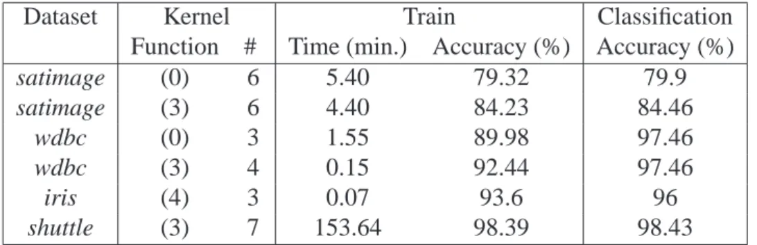
The prototype was tested with several of the most common data sets from the StatLog [47] repository with very good results, as stated in Table2.2.

Dataset Kernel Function Train Accuracy (%) Test Accuracy (%)

dna (1) 98.30 95.62

letter (3) 98.95 95.95

satimage (9) 94.88 90.35

shuttle (7) 99.90 99.85

Chapter 2. Flexible Kernels for RBF Networks 18

Training:

remora.exe 1 A "d:/thesis/dataset/train.csv" 6 1 1

Classification:

remora.exe 1 C output.rem "d:/thesis/dataset/classify-nc.csv" "d:/mestrado/dataset/result.txt" 1

Validation:

remora.exe 1 V output.rem "d:/thesis/dataset/classify-wc.csv" "d:/mestrado/dataset/result.txt" 1

Figure 2.7: Prototype usage example.

Despite the results, unfortunately the prototype was unable for redistribution since it was a very specific stand alone application. It had not been developed to be included, or used by, other applications or frameworks, therefor it had one unique usage and a single specific purpose.

2.5

Improvements

As stated before, the enhancement of the original algorithm, as described in Section2.3, is one of the focus of this dissertation. Several improvements have been introduced, mostly related to the algorithm parameterization.

Despite the changes described here, the original algorithm was preserved unchanged. The only exception is the testing of the spread values, where the increase and the decrease of values are always both tested. Apart from this exception, the resulting implementation, as described in the following Chapter4, allows the use of the original version. In fact, the default configuration reflects the original version of the algorithm.

The enhancements that have been introduced are described in the following sections. Parameterization

One obvious and simple improvement was to allow the user to customize the parameters that were declared static, such as the𝑑 parameter listed in Algorithm2.2. Hence, all pa-rameters that could be defined by the user moved from constants values into user defined values. Namely: (i)𝑑, the initial value of 𝑑; (ii) 𝜀, required by some models; (iii) 𝑛𝑖𝑡𝑒𝑟,

the maximum number of iterations to perform when finding𝑠; and (iv) 𝑛𝑖𝑡𝑒𝑟 𝑐ℎ𝑎𝑛𝑔𝑒𝑠,

the number of iterations without changes that can occur when finding𝑠. Note that the 𝛼

parameter in Algorithm2.2 from the Stage Two of learning procedure in Section 2.3.1, is not parameterized. The reason for such design option came from the prototype results that indicated that the𝛼 parameter could be automatically inferred with very good results,

Chapter 2. Flexible Kernels for RBF Networks 19

iteration occurs from the following formula𝑑 = 𝑑 𝑠𝑡𝑎𝑟𝑡 + 𝑖𝑡𝑒𝑟𝑛𝑖𝑡𝑒𝑟 ∗ (𝑑 𝑒𝑛𝑑 − 𝑑 𝑠𝑡𝑎𝑟𝑡)

where (i) 𝑑 𝑠𝑡𝑎𝑟𝑡 is the initial 𝑑 value; (ii) 𝑖𝑡𝑒𝑟 is the current iteration; (iii) 𝑛𝑖𝑡𝑒𝑟 is, as

seen before, the maximum number of iterations to perform when finding𝑠; and (iv) 𝑑 𝑒𝑛𝑑

is the lower threshold for𝑑, meaning 𝑑 will never be lower than 0.01.

Testing Spread Values

As described in the Stage Two of the learning procedure algorithm, in Algorithm2.2a𝑠′ greater value is tested, but a𝑠′

lower value is only tested if the greater value did not yield a better accuracy value than the one found up to that moment. This has been changed to always test the increase and the decrease of the spread parameter. This means that a lower value will always be tested even if the greater value resulted in a better accuracy than the one found up to that moment.

This is the only modification that cannot be parameterized to allow the execution of the algorithm with the original behavior. This means that the algorithm will always execute using this improvement.

PCA Scale Variance

The Principal Components Analysis (PCA), used for the spectral decomposition, can be scaled to have unit variance before the analysis takes place. The scaling will be performed by dividing the centered columns by their root-mean-square, as Becker et al. states in [2]. In practice, this means that the spectral decomposition will be performed only after all values have been scaled.

Evaluate Each Cluster Individually

In the original algorithm, the classification of a given point is calculated using the sum of the centroid distances per class, as previously described. But it can also be calculated using just the individual centroid distance.

In the original version, the distance of all the centroids is summed per each class, and a point is classified against the distance of the class. With this enhancement, a point can be classified by calculating the distance against an individual class centroid.

Chapter 3

R

This chapter describes R and why it was selected as the target platform for the new im-plementation of the Flexible Kernels for RBF neural networks algorithm. Other solutions have been considered, such as Java1 _{and .Net}2 _{frameworks, but since they have not been}

selected as the target development platform, they are not mentioned here. This chapter also covers the official repository, that holds the packages that can be used to expand R, and the mechanisms provided for development.

3.1

What is R?

R is a programming language, a development framework and a software environment for statistical computing, modeling and data visualization. It was created by Ross Ihaka and Robert Gentleman [27] at the University of Auckland, in New Zealand, and it im-plements the S programming language, developed at Bell Laboratories3 _{by Rick Becker,}

John Chambers and Allan Wilks.

R is currently a GNU4 _{project developed by the R Development Core Team and can}

be regarded as an open source implementation of the S language, providing an easy and accessible route to research in statistics. This makes R very similar to S, it even supports much code from S allowing it to be executed unaltered, and therefor almost all literature targets both systems.

R is a language and cross platform environment that uses a command line interface. Pre-compiled binary versions are provided for various operating systems and there are graphical user interfaces available on some of those systems. It is highly extensible, pro-vides graphical techniques and a wide variety of statistical computing, like linear and nonlinear modeling, classical statistical tests, time-series analysis, neural networks, clas-sification and clustering. Some of R strengths include:

1_{Java is a registered trademark of Sun Microsystems.} 2_{.Net is a registered trademark of Microsoft Corporation.} 3_{Formerly AT&T, now Lucent Technologies.}

4_{GNU is a registered trademark of the Free Software Foundation.}

Chapter 3. R 22

∙ an effective data handling and storage facility;

∙ a suite of operators for calculations on arrays, in particular matrices;

∙ a large, coherent, integrated collection of intermediate tools for data analysis; ∙ support for much S code, allowing it to be executed unaltered;

∙ ease to produce well-designed publication-quality plots, including mathematical

symbols and formulas where needed;

∙ graphical facilities for data analysis and display either on-screen or on hard copy; ∙ an extension mechanism that allows contributions;

∙ a well-developed, simple and effective programming language which includes

spe-cial operators, conditionals, loops, user-defined recursive functions and input and output facilities.

For all the stated reasons, R is widely used for statistical software development and data analysis, making it the de facto standard among statisticians.

3.2

R Language

Due to the similarity between R and S, the R language and its natural evolution follows S. There is a set of books that characterize the language, namely:

1. The New S Language, which is the basic reference for R and was written by Becker

et al. [2],

2. Statistical Models in S, that details the features included in the early nineties and was written by Chambers [7], and

3. Programming with Data, that describes the formal methods and classes of the meth-ods package and was also written by Chambers [8].

Despite these S references, there is a specific R Language Definition [52] that defines the R language. There is also a frequently asked questions (FAQ) [25] that covers the basics and is a good starting point for all new R users.

The language syntax has a superficial similarity with the C programming language, but the semantics are of the functional programming language variety with stronger affini-ties with the Lisp and APL programming languages. In particular, it allows ”computing on the language”, which makes possible to write functions that take expressions as an input, a feature that is common and often useful when applied to statistical modeling and graphics.

Chapter 3. R 23

3.3

R Workspace

The R workspace is the working environment that includes the command prompt and the user defined objects such as vectors, matrices, data frames, lists, functions and variables. This means that the workspace is composed by a working area, that includes all objects currently in memory, and a command prompt where the user can give commands such as (i) a call to any defined function; (ii) a variable manipulation, like an assignment; or (iii) a specific R console command, such as terminate the session or clear the workspace. The management of objects in the workspace memory is dynamic. This means that, for in-stance, a library, function or variable, can be loaded into, or removed from, the workspace at any time.

During a R session, it is possible to save the state of any object from the workspace into an external file, and load it again from the file into the workspace. At the end of a R session, the user can save an image of the current state of the workspace, that includes all the objects, that will be automatically reloaded the next time R is started. It is also possible to save the current workspace state and loaded it at any time. This feature is extremely useful to everyone that needs to keep a restore point or wants to keep a specific state of the current work for sharing or later usage.

R comes with both a command line text console and a graphical console that provides user friendly interaction such as a set of common R console commands and easy access to R packages. There are also other third party R environments that potentiate the usage of R workspace, for instance by combining the console with a script editor. But this is not the only way to interact with R. It is possible to execute an R script by calling the R from the system command prompt and the script as a parameter. That will make R to execute the specified script and, when finished, it will return to the system command prompt.

3.4

Comprehensive R Archive Network

R comes with a set of pre-installed packages that form its basis. In order to expand these basic capabilities, other packages can be obtained from a centralized repository, the Comprehensive R Archive Network (CRAN). CRAN is a family of Internet sites that hold a very wide range of modern statistical packages.

A package is a library, usually about a specific topic, area or functionality, that con-tains a set of functions, data, and the correspondent documentation. The data present in the packages is optional and is usually used to support, test, or illustrate the functions of the package.

Each package expands R by providing new functions to it. The packages are usually available to the scientific community through the R centralized repository CRAN. Obtain-ing and usObtain-ing a package is performed by downloadObtain-ing the package from CRAN and then

Chapter 3. R 24

loading it into the workspace. The graphical console assists the user in this task, making it quite easy and straightforward.

As stated before, one of this dissertation goals is to provide the FRBF, described in the following Chapter 4, as a package in the CRAN repository as a contribution to the scientific community.

3.5

R Development

Simply stated, R allows development through the definition of user functions and class objects. For that, R provides the usual basic programming language mechanisms [52], like control structure, class definition, basic data types, operators, etc.. R is interpreted, which means slower executions when compared with similar compiled code. Nevertheless, using R is actually quite efficient, even when it comes to working with complex operations and large data sets. When packed, a development may be distributed and shared with others.

3.5.1

Objects

R supports two object systems, known as the S3 and the S4 objects.

Simply stated, S3 objects, classes and methods have been available in R since its inception and are very informal. For instance, it is not required to define any data type for its slots, commonly known in Object Oriented Paradigm (OOP) as properties or members. The S4 objects are the new generation that tries to eliminate the weak S3 OOP sup-port. It requires more attention from the developer. In particular, it forces the explicit declaration of slots with a data type and thenew()function must be used to create a S4 object.

3.5.2

Function Overloading

R supports function overloading based on data types. More precisely, a function behavior can be defined based on the data type that it receives as an argument. For instance, the

printfunction, that displays a variable value on the console, changes its behavior de-pending on the variable data type. The printing of a matrix is displayed differently than an integer or an array.

The overloading mechanism is quite simple. R interprets the function name concate-nated with the data type by a dot, preserving the original function signature. Figure3.1

shows how this mechanism can be declared.

This mechanism is very useful when custom implemented classes need a pretty way to display its values to the user.