2015
UNIVERSIDADE DE LISBOA FACULDADE DE CIÊNCIAS DEPARTAMENTO DE INFORMÁTICA
Assessing Pseudogene Expression During Neural
Differentiation by RNA-Seq
Mestrado em Bioinformática e Biologia Computacional
Especialização em Biologia Computacional
Luís Carlos Pereira Simões
Dissertação orientada por: Doutora Ana Rita Fialho Grosso
Instituto de Medicina Molecular
Professor Doutor Francisco José Moreira Couto Faculdade de Ciências da Universidade de Lisboa
i
Agradecimentos
À Doutora Ana Rita Fialho Grosso, não só por me ter orientado de forma excelente no meu trabalho, o que poderá ter sido uma tarefa bastante difícil, mas também por todo o suporte e disponibilidade quer a nível profissional, quer a nível pessoal, que me foi dando ao longo do tempo, o que ficará para sempre marcado na minha mente. Agradeço também pela inspiração profissional que será muito útil no futuro. Ficarei para sempre grato por tudo!
Ao Doutor Sérgio Almeida, Principal Investigador no Instituto de Medicina Molecular, por me abrir a porta do seu grupo de investigação e sempre se ter mostrado disponível e interessado, a todos os níveis. Também por me ter proporcionado conhecer todo um grupo de pessoas fantásticas, o que para mim se complementa com o excelente grupo de investigação a que pertencem e às quais não posso deixar de agradecer pela preocupação que tiveram comigo ao longo deste ano da minha vida e por todo o apoio que me deram. Muito obrigado a todos!
Ao Doutor Nuno Morais por ser uma inspiração a nível pessoal, profissional e desportivo e por sempre se ter mostrado prestável em todos estes campos. Agradeço também pelo espaço e material que me facultou ao longo do tempo. Muito obrigado.
À Doutora Ana Pombo do Max Delbrück Center for Molecular Medicine (Berlim), pela disponibilização dos seus dados para as minhas análises.
Aos meus verdadeiros amigos, por se terem cruzado no meu caminho e terem também vocês moldado um pouco (ou bastante) a pessoa que sou. Por terem acreditado em mim quando eu mesmo duvidei. Por terem sido sinceros ao longo do tempo, mesmo quando isso me magoou. Por todos os momentos de festa, em que todos os problemas e preocupações se apagaram das nossas mentes. Se continuasse aqui a escrever motivos pelos quais agradecer nunca mais parava. Se não fossem vocês e o vosso apoio, todo este ano teria sido muito mais complicado.
Por último, mas não em último, quero não só agradecer mas também demonstrar todo o meu amor e carinho pela minha família, pois esta representa os alicerces de tudo o que construí até agora. Em especial aos meus pais, pois sem vocês nunca estaria aqui e nunca teria tido tantas oportunidades na vida, fruto de muito sacrifício e suor constantes da vossa parte, desde que me lembro de ser gente. Agradeço também toda a dedicação investida na minha educação, e quando falo em educação não tenho em vista apenas o meu percurso académico, mas sim todos os ensinamentos e competências sociais que me foram transmitindo até aos dias de hoje. Eu sei que a vida não tem sido fácil, que nem tudo tem corrido como planeado, mas acredito que depois da tempestade vem a bonança, e se alguém a merece mais que tudo, são vocês. Obrigado por sempre terem lutado por me tornarem o melhor ser humano possível, mesmo quando eu não o quis, mesmo quando não compreendi os vossos pontos de vista, mesmo quando não aceitei os vossos conselhos, mesmo ua do e e oltei po a ha ue algo o fazia se tido… “ei ue tudo o ue fizeram até hoje foi pelo meu bem, mas a evolução advém da diversidade, e isto não só é verdade para a biologia, como para os nossos relacionamentos interpessoais. As nossas diferenças fizeram-me evoluir e continuar no caminho que percorro, acreditando que é o correto. Nunca vos conseguirei agradecer nem retribuir tudo o que fizeram por mim. Resta-me só desejar que vos orgulhe e que isso tenha maior
iii
Resumo
Os pseudogenes são sequências genómicas que foram desprezadas ao longo do tempo, por se pensar que não passavam de réplicas ancestrais de genes codificantes de proteína. Esta visão tem sido desmistificada nos últimos anos e vários estudos têm vindo a surgir mostrando que os pseudogenes não são apenas meras cópias disfuncionais dos genes codificantes de proteína, pois também eles desempenham funções biológicas relevantes.
Existem 14,285 pseudogenes anotados no genoma humano pelo projeto GENCODE (versão 22, Outubro de 2014). O número tem vindo a aumentar ao longo dos anos devido ao desenvolvimento das tecnologias de sequenciação de nova geração (next generation sequencing - NGS) e de algoritmos para identificação de novos pseudogenes. No genoma de ratinho encontram-se anotados 8,526 pseudogenes pelo projeto GENCODE (versão M5, Dezembro de 2014).
A origem destas sequências que derivam de genes codificantes de proteína (genes parentais) dá-se na sua grande maioria por um de dois mecanismos de pseudogenização: duplicação genómica de um locus do gene parental (pseudogene duplicado ou não-processado); ou retrotransposição (pseudogene processado), onde um mRNA é reversamente transcrito em DNA de novo e inserido aleatoriamente no genoma. Este último é o processo pelo qual a maioria dos pseudogenes são originados, levando esta classe a ser a mais estudada. Inicialmente estas sequências podem ser operacionais, mas ao longo do tempo acumulam mutações deletérias que podem resultar na tradução de um codão stop prematuro, ou em mutações frameshift que levam a uma mudança na grelha de leitura, impedindo a expressão bem sucedida destas sequências. Existe ainda uma terceira classe de pseudogenes, os unitários, que não resultam de nenhum tipo de inserções genómicas, apenas de mutações pontuais, le a do assi a ue se to e u ge e estigial .
O primeiro pseudogene foi descoberto em 1977, coincidindo com o aparecimento da primeira técnica de sequenciação. O desenvolvimento das tecnologias de NGS, bem como a redução de custo das mesmas, têm permitido que cada vez mais laboratórios em todo o mundo sequenciem as suas amostras e incorporem a sequenciação de moléculas de DNA (Deoxyribonucleic acid) ou RNA (robonucleic acid) na sua investigação. Uma destas tecnologias é a sequenciação do transcriptoma (RNA-seq) que representa uma forte alternativa ao uso de microarrays no estudo da expressão genética, sendo que para a análise destes dados são essenciais conhecimentos na área da Bioinformática e Biologia Computacional. Esta tecnologia tem permitido o estudo ao nível do transcriptoma não só de genes codificantes de proteína, como de outras sequências nucleotídicas não codificantes. Exemplos disto são os pseudogenes e ncRNAs (non-coding RNAs), permitindo assim compreender que também estes transcriptos não codificantes desempenham um papel importante em termos biológicos. Assim, a ideia de que estas sequências eram apenas zonas do
ge o a se ual ue tipo de i po t ia, se do o side adas li o , tem sido
desmistificada.
Os pseudogenes podem interagir com os seus genes parentais de diferentes formas: fonte de pequenos RNAs de interferência; transcriptos antisense; inibidores competitivos da tradução; RNAs endógenos competitivos; competindo pela ligação a microRNAs partilhados. Apresentam uma expressão específica de tecido para tecido,
iv
sendo que o cérebro e os testículos são os tecidos que apresentam uma maior expressão de pseudogenes. Em 2014 foi descrito o caso de um gene (OCT4A) com um padrão de regulação associado a três dos seus pseudogenes durante a diferenciação neural de células estaminais humanas. Contudo, a extensão de pseudogenes envolvidos na regulação dos padrões de expressão associados com diferenciação nunca foram abordados globalmente. Deste modo, este trabalho tem o propósito de estudar a expressão dos pseudogenes na diferenciação de células estaminais em percursores neuronais, tanto em humano como em ratinho.
De modo a atingir o objetivo, foram analisados dados de transcripoma (RNA-Seq) de amostras obtidas ao longo da diferenciação neural em humano e ratinho. De modo a obter um catálogo completo de pseudogenes foram usadas três bases de dados (Ensembl, Yale e Noncode), perfazendo um total de 19444 pseudogenes no genoma de ratinho e 18061 no genoma de humano. Além disso foi também construída uma pipeline para descobrir novos potenciais pseudogenes, resultando num total de 130 (41 nas amostras de ratinho e 89 nas amostras de humano). Para obter os pseudogenes com expressão diferencial foram testados três métodos implementados em pacotes do R (DESeq e EdgeR), tendo-se optado por usar o pacote EdgeR para a análise final.
Devido à elevada semelhança entre as sequencias do pseudogene e o respetivo gene parental, os alinhamentos contemplaram apenas reads unicamente mapeadas. Assim, foi necessário estudar a mapabilidade dos pseudogenes, percebendo a singularidade dos mesmos e dessa forma filtrar os resultados. Após esta análise foi possível identificar 513 pseudogenes (92 de ratinho e 421 de humano) a variarem ao longo da diferenciação neural. A análise funcional dos respetivos genes parentais revelou 172 pseudogenes, potencialmente interessantes para a diferenciação celular e neural. A comparação dos resultados de ambos os organismos identificou um dos novos pseudogenes de ratinho como homólogo de um pseudogene humano anotado e contendo o ortólogo gene parental (FAM205A).
De modo a explorar a regulação dos genes parentais pelos seus pseudogenes, foi avaliada a correlação dos níveis de expressão para cada par de pseudogene-parental, sendo que em ambos os organismos foi encontrado um elevado número de pares de genes positivamente correlacionados.
Neste estudo, foram ainda incluídos os resultados com dados de transcriptoma ao nível de célula-única (single-cell). Devido ao nível baixo de sequenciação dos dados de célula-única a percentagem de pseudogenes expressos (com contagens processadas) foi reduzida e não permitiu detetar os pseudogenes da análise de transcriptoma global. Contudo, a análise destes dados revelaram quatro pseudogenes diferencialmente expressos cujos parentais têm funções relevantes a nível da diferenciação neuronal e envolvidos nas vias de sinalização de doenças neurodegenerativas.
Concluindo, o presente trabalho permitiu obter um conjunto de pseudogenes que variam ao longo da diferenciação neural e com o potencial para regularem genes parentais associados com diferenciação celular, neural ou doenças neurais. Além disso, os resultados realçam a importância da utilização de dados das tecnologias de sequenciação em larga-escala na descoberta de novos transcritos.
Palavras chave: pseudogene; pseudogenização; RPKM; diferenciação neuronal; RNA-Seq
v
Abstract
Pseudogenes are nucleotide sequences that were been neglected since they were discovered. In the last years this point of view is changing, and their functions have been studied and there are been annotated more pseudogenes than the estimated number in human genome.
Pseudogenization process can occur essentially by two mechanisms: genomic duplication of a parental gene locus (duplicated pseudogene); or retrotransposition (processed pseudogene) where an mRNA is reversely transcribed and randomly inserted in the genome. Initially these type of sequences can operate as a normal protein coding gene, but after some time and accumulation of deleterious mutations the open reading frame is modified, preventing their well-succeeded expression.
RNA-Seq technology allows studying the transcriptome of all type of biologic sequences, not only protein coding genes, giving an idea of the roles performed by them and de stif i g the idea that the a e ge o i ju k .
There are evidences of interaction with their parental genes as: source of endogenous siRNAs; antisense transcripts; competitive inhibitors of translation; competitive endogenous RNAs (ceRNAs); competing for binding to shared miRNAs. In 2014 (last year) was described that a protein coding gene (OCT4) with a regulation patern associated with three of its pseudogenes in human stem cells differentiation.
To achieve our goal, were analyzed transcriptome sequencing (RNA-Seq) of neural differentiation datasets of human and mouse. Three databases were merged and a pipeline was constructed in order to find new possible pseudogenes, resulting in a total 130 in two dataset. Differential expression analysis was performed with two R packages (DESeq and EdgeR) with three different approaches, and after comparison, EdgeR pair wise analysis was selected as the best for our study.
Because of the high similarity between pseudogenes and their cognates, we only allowed reads uniquely mapped. Thus, it was necessary to study mappability of pseudogenes, realizing the uniqueness of them and therefore filter results. After this analysis, was possible to identify 513 pseudogenes varying along differentiation (92 in mouse dataset and 421 in human dataset). Functional analysis allowed to identify 172 potentially interesting pseudogenes in neural differentiation. Comparison of results between organisms identified one new putative mouse pseudogene homologous of anannotated pseudogene in human, with an ortholog parental (FAM205A).
To assess regulation of cognates by their pseudogenes, expression values were e aluated ith Pea so ’s oeffi ie t a d the e e e fou d a pai s ith sig ifi a t correlation.
Processed data from single-cell experiments were analyzed too and there were
highlighted four differentially expressed pseudogenes associated with
neurodegenerative diseases and neural differentiation.
Finally, this work enabled to obtain a set of pseudogenes varying along neural differentiation with regulatory potential of parental genes associated with cell and neural differentiation or neurodegenerative diseases. The results highlight the importance of high throughput sequencing in discovery of new transcripts.
vii
Index
1. Introduction ... 1
1.1. Next generation sequencing ... 1
1.1.1. Technologies... 1
1.1.2. Applications ... 2
1.1.3. RNA-Seq overview ... 3
1.2. Pseudogenes ... 4
1.2.1. Origin ... 5
1.2.2. Regulation of cognate genes ... 6
1.2.3. Roles in neural differentiation ... 7
1.3. Objectives ... 7
2. Methods ... 8
2.1. RNA-Seq Data and Preprocessing... 8
2.2. Reads alignment ... 8
2.3. New pseudogenes discovery ... 9
2.4. Reference genome annotation ... 10
2.5. Gene summarization and normalization ... 10
2.6. Unsupervised analysis ... 11
2.7. Gene expression analysis ... 11
2.8. Pseudogenes Mappability ... 12
2.9. Pseudogenes vs. parental genes ... 13
2.10. Functional/Pathway enrichment analysis ... 13
2.11. Species Comparison ... 14
2.12. Single-cell data comparison ... 15
3. Results and discussion ... 16
3.1. RNA-Seq Data Preprocessing... 16
3.1.1. Data quality ... 16
3.1.2. Alignment ... 16
3.2. Identification of New Pseudogenes ... 17
3.3. Unsupervised Clustering Analysis... 19
3.4. Comparison of Statistic Methods for Differential Expression Analysis ... 21
3.5. Differential Expression Analysis and Pseudogene Mappability ... 23
viii
3.7. Species Comparison ... 29
3.8. Comparison with Single-Cell Data...30
4. Conclusions ... 33
ix
List of Tables
1.1. GENCODE project annotated pseudogenes 5
2.1. Merged annotations 10
3.1. Alignment summary 17
3.2. New pseudogenes discovered 18
3.3. Pseudogenes troubleshooting summary 26
3.4. Functional/Pathway analysis 28
3.5. New mouse pseudogene orthology analysis 31
x
Supplementary Tables
1. Human new putative pseudogenes 2. Differentially Expression Analysis
3. Expression values for pseudogenes which cognates have relevant functions 4. Correlation between pseudogenes and their cognates
xi
List of Figures
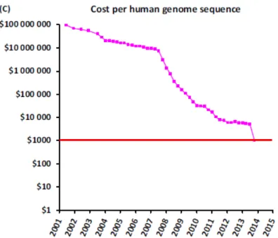
1.1. Evolution of cost per human genome sequencing 2
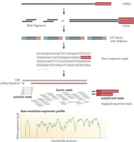
1.2. Summarization of a RNA-seq experiment 4
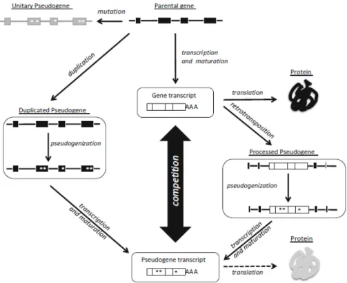
1.3. Schematization of pseudogenization processes 6
2.1. Schematic view of workflow to identification of new pseudogenes 10
2.2. UCSC Genome Browser mappability track example 13
2.3. Example of correlation plot between pseudogene and its parental 13
2.4. Ensembl Biomart orthology analysis summarization 14
3.1. Per base quality example plots 16
3.2. UCSC Genome Browser tracks for new pseudogene examples 19
3.3. Unsupervised clustering analysis of pseudogenes 20
3.4. Unsupervised clustering analysis of protein coding genes 21
3.5. Gene expression analysis summarization for three distinct methods 22
3.6. Venn Diagrams comparing all methods 22
3.7. Fold change comparison 23
3.8. Example of expression view 24
3.9. UCSC Genome Browser example tracks for low covered DEP 25
3.10. Expression summary using EdgeR package 26
3.11. Filtered DEP expression summary 27
3.12. Filtered mouse DEP with relevant functions heatmap 29
3.13. Filtered human DEP with relevant functions heatmap 30
3.14. UCSC Genome Browser tracks for a new mouse pseudogene 31
3.15. Box plots of DEP in Single-Cell data expression values 32
xiii
List of abbreviations
ceRNA – competitive endogenous RNA DEA – Differential Expression Analysis DEG – Differentially Expressed Gene DEP – Differentially Expressed Pseudogene DNA – Deoxyribonucleic Acid
ds-RNA – double-strand RNA
endo-siRNA – endogenous small inferring RNA ESC – Embryonic Stem Cell
FC – Fold-Change
FDR – False Discovery Rate
GEO – Gene Expression Omnibus
miRNA – micro RNA mRNA – messenger RNA
NGS – Next-Generation Sequencing
NOS – Nitric Oxide Synthase NPC – Neural Precursor Cell OR – Olfactory Receptor
PCA – Principal Component Analysis PCR – Polymerase Chain Reaction
PGM – Personal Genome Machine
RNA – Ribonucleic acid RNA-Seq – RNA sequencing
RPKM – Reads Per Kilobase per Million RPM – Reads Per Million
SRA – Sequence Read Archive
SMRT – Single Molecule Real Time sequencing TPM – Transcripts Per Million
UCSC – University of California Santa Cruz UTR – Untranslated Reagion
1
1.
Introduction
1.1.
Next Generation Sequencing
1.1.1.
Technologies
In 1944 DNA (Deoxyribonucleic acid) was described as genetic material by Oswald Theodore Avery. Nine years later (1953) Watson and Crick determined the structure of DNA as we know nowadays, a double-helix structure, defined by sequences of four nucleotide bases. These events were crucial to the evolution of molecular biology and they led scientific community to go deeper in the understanding of the. In order to make it happen, there was a need to achieve a method that could sequence and tell us the order that those bases appear in specific DNA sequences or in entire genome.
The first step in sequencing technologies was driven by Sanger, with the de elop e t of a fi st ge e atio te h ology based on chain-termination method (Sanger et al., 1977), able to determine which base is in a specific position of a certain region of genome. This method was used worldwide and represents a revolutionary technique that allowed scientists to understand more and more about DNA.
Since 1977 until now, a lot of techniques were develop and the first automatic sequencing machine (AB370) appear ten years later, developed by Applied Biosystems, based on capillary electrophoresis technique, allowing a faster and more accurate
se ue i g, te yea s late f o “a ge ’s dis o e y Liu et al., . The ai goals
after this turning point in the sequencing technology were increasing speed and accuracy while reducing cost. This became more evident with the Human Genome
P oje t . To a hie e that e e de elop se e al se o d ge e atio se ue i g
technologies - Next Generation Sequencing (NGS).
The first NGS technology commercialized was Roche 454 (2005), followed by Solexa/Illumina (2006) and SOLiD (2007) (van Dijk et al., 2014). Steps of fragmentation and amplification by Polymerase Chain Reaction (PCR) of genetic material are required in this type of sequencing before detection of specific nucleotides using fluorescence and camera scanning. In 2010, Ion Torrent released the Personal Genome Machine (PGM) that uses semiconductor technology instead of fluorescence. More recently,
new technologies emerged ( alled thi d ge e atio ) that allow the sequence in real
time of single molecules without previous DNA amplification. One of the most used third generation methods was developed by PacBio in 2010 (van Dijk et al., 2014).
Although very expensive, the cost of sequencing using NGS has been decreasing along the past years (Figure 1.1) giving us great perspectives that these technologies will be even more reachable worldwide.
2
1.1.2.
Applications
Evolution and wide availability of NGS technologies allowed, over the past decade, the development of several assays to answer different biological questions, focused on: transcription; translation; replication; post-transcriptional modifications; methylation; nucleic acids interactions; chromatin structure.
RNA-Seq (RNA sequencing) is the most widely used method to study
transcription. In this methodology a population of RNA is converted to cDNA fragments (library preparation) with adaptors attached to one or both ends, and the sequenced (Wang et al., 2009). There are many other technologies focused on transcription. With
NET-Seq (Native Elongating Transcript Sequencing) is possible to monitor transcription
at u leotide esolutio , y deep se ue i g ’ e ds of as e t t a s ipts (Churchman et al., 2011). In 3P-Seq (Poly(A)-Position Profiling by Sequencing) application, a RNA:DNA oligonucleotide is hybridized with thymines and ligated to the mRNA polyadenylated tail to prevent internal priming (Jan et al., 2011). GRO-Seq (Global Run-On Sequencing) methodology is applied to map position, amount, and orientation of transcriptionally engaged RNA polymerases by nuclear run-on RNA molecules (Core et al., 2008).
For determine chromatin structure the number of methodologies possible to use is very large. In FAIRE (Formaldehyde-Assisted Isolation of Regulatory Elements) assays, chromatin and formaldehyde are cross linked in vivo, and together with massive parallel sequencing (FAIRE-Seq) is a methodology used to study the relationship between chromatin structures (Giresi et al., 2007; Yang et al., 2013). For mapping DNase I hypersensitive sites, DNase-Seq (DNase I Hypersensitive Sites Sequencing) is a method that selectively digests nucleosome-depleted DNA followed Figure 1.1.: Evolution of cost per human genome sequencing. Graphic from van Dijk et al., 2014. Red line represents the 1000$ cost threshold per human genome sequence, one of the goals achieved.
3
by high-throughput sequencing (Song and Crawford, 2010). These two technologies a e used to fi d ope h o ati egio s ith egulato y a ti ity o espo di g to nucleosome-depleted regions (NDRs) (Song et al., 2011). With ChIA-PET (Chromatin Interaction Analysis by Paired-End Tag Sequencing) is a method for studying long-range chromatin interactions in a three-dimensional mode and provides a more trustworthy way to determine transcription factor binding sites and identify chromatin interactions (Li et al., 2014).
An important question in biology is the manner how proteins interact with nucleic acids. ChIP-Seq (Chromatin Immunoprecipitation Sequencing) is widely used to study protein-DNA interactions. It allows mapping genomic locations of transcription factors binding and histone modifications, after a protocol of chromatin immunoprecipitation and high throughput sequencing (Stephen et al., 2012). Focused on protein-RNA interactions, CLIP-Seq (Cross-Linking Immunoprecipitation) is an effective strategy by stringent purification of RNAs bound to a protein of interest in living cells (Murigneux et al., 2013).
In methylation studies BS-Seq (Bisulfite Sequencing) allows to measure cytosine methylation on a genome-wide scale within specific sequence contexts after bisulphite treatment of DNA (Cokus et al., 2008).
Translation is other of the biological questions that massive sequencing allows to understand. The basis of another NGS application, Ribo-Seq (Ribosome profiling), is the isolation of messenger RNA (mRNA) fragments protected by ribosomes followed by massively parallel sequencing. This methodology allows us to measure ribosome density along all mRNA transcripts (Michel et al., 2014).
In the next subchapter RNA-Seq methodology is more detailed, because is the one used in our study.
1.1.3.
RNA-Seq overview
RNA sequencing (RNA-seq) is a NGS method specially developed for characterization and quantification of the transcriptome. First, it is necessary a construction of cDNA fragments library, from a RNA population, with adaptors atta hed to the se ue e’s e ds. Each molecule is sequence (an amplification step may be necessary) resulting in millions of single-end or paired-end (RNA fragments sequenced from one end or both ends, respectively) as demonstrated in Figure 1.2 (Wang et al, 2009).
Paired-end sequencing is more efficient dealing with multi-mapping which can be a serious problem at the alignment step, because both ends of each cDNA fragment should map nearby on the transcriptome, allowing solving this type of ambiguity in most part of the times, unlike single-end reads.
This method has many advantages when compared with microarrays hybridization-based approaches that had been the most widely used methodology to quantify the transcriptome. Specially, RNA-Seq shows higher sensitivity and dynamic range and lower technical variation (Oshlack et al., 2010). Furthermore, the technology does not require a previous knowledge of existing genomic sequences, unlike microarrays methodology, making RNA-Seq an interesting method to detect transcripts in non-model organisms (Wang et al, 2009).
4
Figure 1.2: Summarization of a RNA-Seq experiment. Figure from Wang et al., 2009.
1.2.
Pseudogenes
The first pseudogene was discovered by Jacq and colleagues (1977), for the oocyte-type 5S RNA gene in the genome of a model organism, Xenopus laevis. Since then, pseudogenes have been described as a relic of evolutionary selection by the scientific community (Muro et al., 2011).
Only some years after, Korneev and colleagues (1999) identified the first pseudogene with a relevant biological function, suggesting that the nitric oxide
synthase (NOS) pseudogene transcript acts like an antisense regulator of neural NOS,
its parental.
Due to the development of new approaches, several functional pseudogenes have been described for the past years, demystifying the idea that pseudogenes ep ese t a atego y of ju k-DNA o ge eti fossils . This topic will be discussed in the next subchapters.
With the emerging knowledge of pseudogenes and their functions, arises the need to identify and annotate them genome-wide. Three years ago, GENCODE using simulations estimated that human genome contains, approximately 14000 pseudogenes (Pei et al., 2012). Now, GENCODE has more than 14000 pseudogenes
5
(Table 1.1) and with the evolution of sequencing technologies and analysis methods, this number is expected to increase.
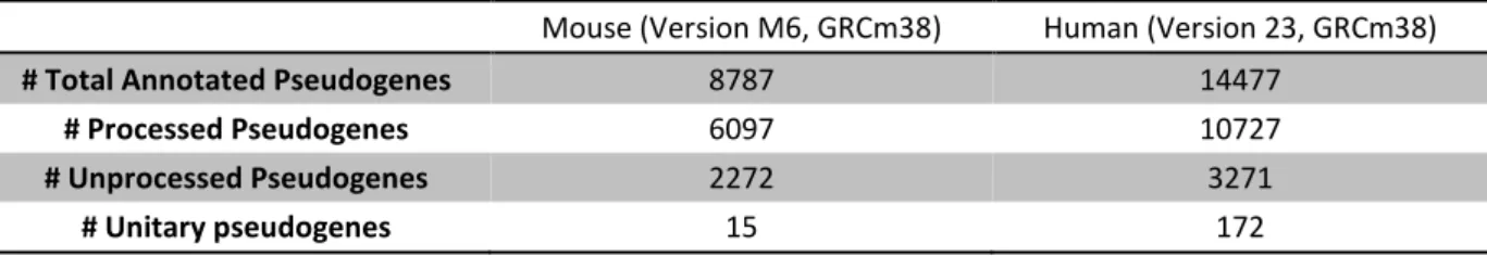
Table 1.1.: GENCODE project annotated pseudogenes summarization for mouse and human genomes. Data obtained from the GENCODE site (gencodegenes.org/) on 13rd August 2015.
Mouse (Version M6, GRCm38) Human (Version 23, GRCm38)
# Total Annotated Pseudogenes 8787 14477
# Processed Pseudogenes 6097 10727
# Unprocessed Pseudogenes 2272 3271
# Unitary pseudogenes 15 172
1.2.1.
Origin
Pseudogenes can be divided into some categories, depending on its origin. Essentially, there are three classes of pseudogenes: processed, duplicated and unitary (Pei et al., 2012). The first two classes are derived from genomic insertion events, while the third one just depends on accumulation of punctual mutations on the pa e tal ge e u leotide se ue e, leadi g to a estigial ge e .
Duplicated pseudogenes derived from incomplete gene duplication events in a
cell, as indicated by their names, usually in a near locus of the parental gene. This pseudogene suffers a pseudogenization process, losing its function as protein coding gene (Mighell et al., 2000).
Processed pseudogenes are the most studied class of pseudogenes, and a
reason why that happens is because they are the most abundant. Their formation is originated by the reverse transcription of a mature mRNA (already spliced) back into DNA that is randomly inserted into the genome. Because of that, they lack promoter a d i t o s a d typi ally ha e ’UTR u t a slated egio a d poly-A tails. Normally these pseudogenes are found on different chromosomes of parental gene (Torrents et al., 2003; Pei et al., 2012).
Figure 1.4 summarizes the different pathways to generate a pseudogene
starting from a protein coding gene (parental) for each class of pseudogene.
Curiously, the olfactory receptors (OR) genes is one of the families more pseudogenized in humans (Olender et al., 2008; Niimura, 2009). It was hypothesized that this phenomenon was related with the development of vision and decreasing of odor sensing. Olfactation results from the combination of different ORs, thus the use of pseudogenes to modify OR genes could be less dispendious (Olender et al., 2008).
6
Figure 1.3: Pseudogenization processes for different classes of pseudogenes, deriving from a protein coding gene (parental gene). Figure from Laura Poliseno, Functions and Protocols, Pseudogenes book (2014).
1.2.2.
Regulation of cognate genes
Pseudogenes can regulate their cognates (parental genes) by some different ways: antisense transcripts; competitive inhibitors of translation; source of
endogenous small inferring RNAs (endo-siRNAs); competitive endogenous RNAs
(ceRNAs).
The first evidences that pseudogenes regulate their cognates are from 1999, when it was understood that the antisense region of a pseudogene transcript prevented the mRNA translation of the respective parental (Korneev et al., 1999).
Connexin43 pseudogenes can inhibit their parental expression while they are
expressed (Kandouz et al., 2004), acting as competitive inhibitors of translation. Transcripts of pseudogenes can form double-strand RNAs (dsRNAs) by interacting with mRNAs resulting from protein-coding genes and then processed into
endo-siRNAs (Tam et al., 2008).
Some transcribed pseudogenes, because of the high similarity with their cognate genes appear to be strong ceRNAs (Welch et al., 2015). Thus, most of the transcribed pseudogenes can regulate their parental genes by competing for miRNA biding (Poliseno et al., 2010).
The processes that lead regulation of protein coding genes by their pseudogenes are still being explored and described. The understanding of these genomic regions previously believed ge eti fossils e ol ed i the last yea s a d tends to increase with more studies focused on them.
7
1.2.3.
Roles in neural differentiation
Neural differentiation from embryonic stem cells advances are very promising for nervous system therapies and neural tissue repair (Abranches et al., 2009) and it is a potential strategy for neurodegenerative diseases treatment (Felfly et al., 2011). Neural differentiation resulting in NPC formation shows specific regulation and gene expression patterns for clusters of genes (Zimer et al., 2011).
Pseudogene expression is tissue-specific, with testis and brain showing the highest levels of their transcription (Soumillon et al., 2013). Recent findings suggest that pseudogenes may play functional role on neural differentiation. For instance, the pluripotency regulator OCT4 is a transcriptional activator of genes involved in maintenance of undifferentiated state and as a repressor of differentiation-specific genes. Notably, expression of OCT4 and of its several pseudogenes was found to follow a developmentally regulated pattern in differentiating human embryonic stem cells (ESCs), suggesting that a tight regulatory relationship between them drives specific cellular functions (Jez et al., 2014). Pseudogenes widespread expression gives clues that these sequences may play also an important role in cancer, being some of them cancer-specific (Kalyana-Sundaram et al., 2012).
1.3.
Objectives
Transcriptomic alterations during cell differentiation have been extensively characterized for protein-coding genes and non-coding RNAs, however the changes of other classes of non-coding genes, such as pseudogenes, have been largely unexplored. Hence, we decided to identify putative pseudogenes involved in neural differentiation and to assess their pattern conservation between different species.
Specifically, this works aims to:
1. Identify potentially new pseudogenes transcribed during neural differentiation; 2. Characterize the pseudogene transcriptome and determine the significant
expression alterations;
3. Determine the functional role of pseudogenes, by monitoring the expression of the parental genes and their involvement in pathways relevant for neural differentiation;
4. Assess the conservation of pseudogene regulatory patterns between species. To assess this, we will use RNA-Seq data obtained from different stages of
embryonic stem cells (ESCs) differentiation into neural precursor cells (NPC), for
8
2.
Methods
2.1.
RNA-seq Data and Preprocessing
The present work involved the analysis of RNA-seq datasets for two different organisms, mouse and human. We gathered whole-transcriptome data from different stages of neural differentiation of mouse embryonic stem cells (ESCs) through collaboration with Dr. Ana Pombo from the Max Delbrück Center for Molecular Medicine (Berlin). Sequenced samples were collected for 5 time points (days 0, 1, 2, 3 and 4) along differentiation of ESCs to neural percursors (NPs) as previously described (Abranches et al., 2009). Transcriptomic data for human differentiation was recently published (Sauvageau et al., 2013) and was obtained from Gene Expression Omnibus (GEO) database (http://ncbi.nlm.nih.gov/geo/, Acc.Number GSE56785). Samples from NPC induced differentiation from stem cells, were collected over 7 time points (days 0, 1, 2, 4, 5, 11 and 18) assayed in triplicate cultures. Both transcriptomes contained paired-end sequencing reads with 100 bp (mouse) and 101 bp (human).
The first step of preprocessing, consisted in the conversion of the files downloaded from GEO in .sra format to .fastq, using the SRA (Sequence Read Archive)
Toolkit, as showed by the following command:
fastq-dump --split-files GEODownloaded.sra.
Fastq-dump command with --split-files option allows converting a .sra file to two .fastq format files, with matched mate-pair reads.
Second, data quality was assessed using FASTQC tool over .fastq files. This tool evaluates the quality of NGS data for the following characteristics: duplication levels;
k-mer profiles; per base GC content; per base n content; per base quality; per base
sequence content; per sequence GC content; per sequence quality; sequence length distribution.
2.2.
Reads alignment
Paired-end reads were aligned against mouse and human reference genome (mm10 and hg19, respectively) with TopHat2 (Kim et al., 2013), allowing 2 hits maximum and with a 100 bp mean distance between mates and a 50 bp standard deviation, as demonstrated in this example:
tophat2 -g 2 fusion-search mate-inner-dist 100 mate-std-dev 50 --output-dir OutputDirectory --GTF KnownTranscriptomeFile.gtf
Bowtie2Index InputFile1.fastq InputFile2.fastq.
Since pseudogenes have high similarity with their cognates, the same read can align perfectly to both genes. Hence, to avoid this technical bias and assign each read correctly, only uniquely aligned reads were considered for downstream analyses. Thus,
9
after alignment reads mapped more than once were excluded, keeping only reads with NH:i: flag i .bam output files.
2.3.
New pseudogenes discovery
To assess the pseudogene expression profiles, along the last years there were designed several pipelines to identify new pseudogenes. Here, we aim also to detect new putative pseudogenes expressed along neural differentiation.
The method used to identify potential novel pseudogenes was based on two pipelines developed before (Kalyana-Sundaram et al., 2012; Zheng and Gerstein, 2006) and its schematically view represented in Figure 2.1. First, uniquely mapped reads were sorted by read name with samtools sort tool. Second, bedtools pairtobed tool was used to establish which paired-end reads do not intersect with annotated regions in neither ends and are located in the same chromosome, as showed by the command: pairToBed -abam SortedFile.bam -b KnownRegionExonsFile.bed -type
neither -bedpe | awk '$1==$4' - > OutputFile.bedpe.
This step created a .bed file with the coordinates for each paired-end read located in intergenic regions. Next, the duplicated reads were removed. Then, the overlapping paired-end fragments are clustering using bedtools merge tool. Finally, only clusters longer than 40 bp, shorter than 5000 bp, taking into account that less than 10% of our human annotated pseudogenes are bigger than this threshold and supported by more than 1000 paired-end reads were selected:
sort -V -k1,1 -k2,2 PairRangeFile.bed | awk '!x[$1,$2,$3]++' - | mergeBed -i stdin -c 6,1 -o distinct,count | awk '$5>100' - | awk ' $3-$2>40' - | awk 'BEGIN{FS=OFS= \t } {print $1,$2,$3, $1 "_" $2 "_" $3, $5, $4}' - > MetaClustersFile.bed.
Then, we proceed to the identification of the putative parental genes for the discovered pseudogenes. First, we obtained the meta-clusters sequences using
bedtools getfasta:
fastaFromBed -name -fi ReferenceGenome -bed
FinalMetaClustersFile.bed -fo FinalMetaClustersFile.fasta.
Since the sequence was determined, BLAT (Kent, 2002) against annotated protein coding genes was performed to determine putative parental genes for these meta-clusters, filtering the results with a similarity higher than 95% and a E-value lower than 1E-4.
After all, we obtained a .gtf file with the coordinates of the potential pseudogenes for each sample that were merged to obtain a single annotation file with all new discovered pseudogenes.
10
2.4.
Reference genome annotation
The reference gene annotations used in further analyzes for both organisms are result of compilation and merging of all exons transcripts from three databases,
Ensembl, Yale and Noncode. Versions of each annotation are Ensembl 75, Yale 74 and
Noncode V4u1 for human (hg19 assembly) and Ensembl 76, Yale 76 and Noncode V4 (mm10 assembly). For Noncode V4 annotation was necessary to do a LiftOver step from mm9 assembly to mm10.
For downstream analysis, the new pseudogenes were concatenated to the reference genome annotation.
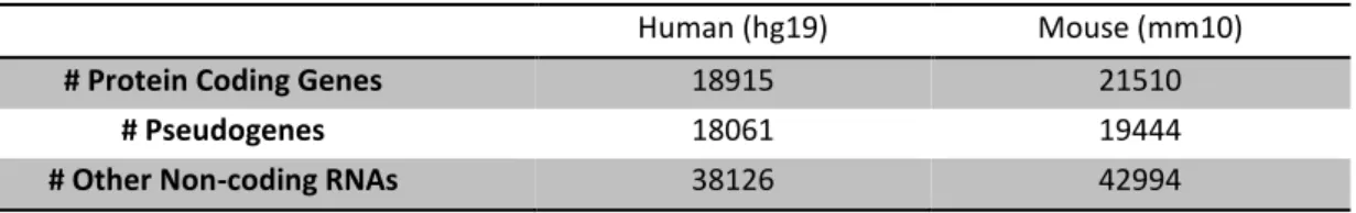
Table 2.1.: Summarization of merged annotations in human and mouse.
Human (hg19) Mouse (mm10)
# Protein Coding Genes 18915 21510
# Pseudogenes 18061 19444
# Other Non-coding RNAs 38126 42994
2.5.
Gene summarization and normalization
In order to determine the expression levels of each transcript, bedtools
multicov tool was run for all .bam files:
11
bedtools multicov -split -bams File1.bam File2.bam (…) FileX.bam -bed MergedAnnotation.gtf > multicovOutputFile.txt.
This command results in a tab delimited .txt file, where the first columns are equal to .gtf file given as input, but with more X columns, being X the number of .bam files or, in other words, the number of samples.
Next, read counts were normalized calculating RPKM (reads per kilobase per million) for each gene in each sample, a measure to estimate gene expression, following this formula: RPKM = (10^9 * C)/(N * L); where C represents the number of reads mapping a gene, N the total number of reads and L the exon length for a gene, in a specific sample. This normalization step takes into account biases within lane (scaling for gene length) and between lane (adjust for total number of reads) and it was used for following unsupervised analyses (Section 2.6).
To normalize read counts for gene expression analysis (Section 2.7) within lanes and between them was used an R package, EDASeq, because R packages do not accept RPKM values.
2.6.
Unsupervised analysis
Exploratory analysis of RNA-Seq data usually involves unsupervised analysis to find hidden patterns or grouping data. One of the methods often used is hierarchical
clustering. This method consists in an algorithm that agglomerates the data by a
specific distance method chosen, ordering (n-1) subtrees, where n is the number of samples. Practically, the Euclidean distance between the RPKM values of each sample are estimated using dist() R function. Then, the distance matrix is submitted to hclust() function, to obtain the cluster dendogram graphical representation.
Other technique to achieve this is principal component analysis (PCA). PCA is a dimensionality reduction method, resulting into a new coordinate system where the first axis corresponds to the first principal component (PC). PCs are a new set of variables that can be interpreted as the direction that resumes the variation among them. The first few PCs normally capture most of the variation in original data, and the last fe o ly aptu e oise Yeu g a d Ruzzo, . For this analysis the RPKM values were first standardized using the stdize() R function, implemented in pls package. Then, the standardized matrices were submitted to princomp() R function.
These two analyses were performed splitting pseudogenes and protein coding genes, in order to compare clustering of samples with different features.
2.7.
Gene expression analysis
As pseudogenes are very low expressed compared to their cognates, there was a need to compare several methods to perform differential expression analysis (DEA). Th ee ethods e e pe fo ith ouse’s dataset, with two R libraries, EdgeR
12
(Robinson et al., 2010) pairwise comparison and DESeq (Anders and Huber, 2010) time
series analysis and pairwise comparison, where data is modeled as negative binomial
distributed.
EdgeR pairwise comparison consists in using this R package estimateGLMCommonDisp() function to estimate negative binomial dispersion parameter for our gene expression datasets. Next, using glmFit() function and dispersion calculated we fitted a negative binomial generalized log-linear model for our counts. Finally, with fitted model, a statistical test is performed with glmLRT() function, for each day against day 0 of differentiation.
DESeq time series analysis uses fitNbinomGLMs() function to fit the generalized
linear model of our counts dataset for the two hypothesis: fits to the formula that the time course is a covariate or fits the null hypothesis. Then, p-values where calculated with nbinomGLMTest() function, correcting this values with p.adjust() function.
The last method, DESeq pairwise comparison of read counts only uses nbinomTest() function for all days against day 0 of differentiation.
The comparison of these three methods is presented in chapter 3.
2.8.
Pseudogenes Mappability
The use of uniquely aligned reads to avoid fragments mapping to multiple similar regions, such as pseudogenes and their cognates, will create a bias in the mappability of pseudogenes. Hence, the pseudogenes with high similarity to the parental genes will have long regions without reads aligned (i.e, unmappable). Thus, these pseudogenes will have false low expression values due the normalization of the read counts by the total gene length.
To overcome this problem we assessed the mappability/uniqueness analysis for pseudogenes loci. Resuming, this analysis consists in the alignment of the pseudogenes sequences, which were fragmented in k-mers of the original reads length. So, a .gtf file with k-mers of 100 nt was created for all pseudogenes annotated in mouse genome (extending 100bp upstream and downstream from annotation). For human genome, the process was the same but with 101nt (because reads have 101bp). Then these sequences were passed to .fasta format with bedtools getfasta tool and aligned to the reference genome with bowtie2 tool. Non-unique aligned reads were excluded from the output .bam file and a bedgraph was generated with bedtools genomecov tool:
genomeCoverageBed -ibam UniquelyMapped100mersFile.sam -g GenomeFile.txt -bg -split -scale 0.01 >> Unscaled.bedgraph.
The bedgraph was submitted to UCSC Genome Browser in .bw format and this track can be visualize as shown in Figure 2.2. Regions with higher mappability will represent unique regions in the genome, with maximum value being one.
13
Figure 2.2.: UCSC Genome Browser mappability example track of pseudogene ENSMUSG00000083548.
Mappability varies significantly between different genomic regions, so we should take this in account especially for pseudogenes. Thus, we considered for analysis only the pseudogenes with mappability higher than 0.5 in at least 50% of total gene length.
2.9.
Pseudogenes vs. parental genes
As discussed previously
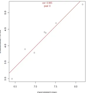
pseudogenes can regulate their cognates by some different ways (Section 1.2.2). To investigate this hypothesis, we compared the expression patterns of pseudogene and respective parental along neural differentiation. Thus, we performed a
correlation test for each pair
pseudogene/cognate using logarithmic
RPKM values (log2) and Pearson’s
coefficient method implemented in cor.test() R function. Then, p-values were corrected for multiplicity problem using
False Discovery Rate approach
implemented in p.adjust() R function.
Finally, for each pair
pseudogene/cognate with a significant correlation was produced a scatter plot,
showing the expression for the
pseudogene and respective parental gene (example in Figure 2.3).
2.10.
Functional/Pathway enrichment analysis
To assess which functions and pathways were significant altered during neural differentiation, we performed an enrichment analysis using DAVID’s functional
annotation tool (Huang et al., 2007). We performed the analysis for all the genes
differentially expressed and also for the parental genes of the pseudogenes with significant expression alterations.
Figure 2.3.: Example of Correlation between pseudogene and its parental plot. In this case genes are positively correlated.
14
For the analysis and functional assignment we used the following annotations: Gene Ontology Term for Biological Process (GOTERM_BP_FAT); Gene Ontology Term for Molecular Function (GOTERM_MF_FAT); Kyoto Encyclopedia of Genes and Genomes pathways (KEGG_PATHWAY).
Enrichment pathway analysis was performed with DAVID Functional Annotation Chart tools, using Fisher Exact statistics and default parameters. Only pathways/functions with Be ja i i’s o e ted p-value lower than 0.05 were selected.
To identify the differentially expressed pseudogenes functionally relevant in neural differentiation, we assessed the function of respective parental genes. First, the DAVID Functional Annotation Table tool was used to obtain the function and pathways for each parental gene. Second, we searched for terms related to neural differentiation, cell differentiation, cell cycle and neurodegenerative diseases.
To visualize the expression patterns of functional relevant
pseudogene/parental gene pairs, there were produced heatmaps with variations (log2
fold-change) of pseudogenes differentially expressed and their respective cognates using heatmap() R function. The colors used in these heatmaps were created with brewer.pal() function from RColorBrewer package.
2.11.
Species Comparison
Orthologs are genes evolved from a common ancestral by speciation and generally have the same function between species.
In order to identify conserved pseudogenes altered consistently in mouse and human neural differentiation we performed two different approaches. First, we compared the parental genes for which pseudogenes showed significant expression alterations along cell differentiation. We used
Ensembl Biomart tool (ensembl.org/biomart/) to identify the
orthologous genes between mouse and human. Figure 2.4 shows the filters and attributes used. The output reports, for
ea h ouse’s pa e tal ge e E se l ID, the espe ti e
human Ensembl ID, the common ancestor, percentage identities with query gene and human gene and a binary value of orthology confidence. Only gene pairs with an orthology confidence value equals to one were considered.
Second, we used liftOver tool from UCSC Genome
Bioinformatics to identify homologous regions of the
pseudogenes between different organisms. This was
performed to convert the genomic coordinates of new pseudogenes discovered and annotated DEP in mouse dataset to human genomic coordinates and vice versa. The results from coordinates conversion were submitted to bedtools intersect tool in order to compare these converted positions against the genes annotated in the other organism.
Figure 2.4: Ensembl Biomart orthology analysis summarization. Printed from Ensembl Biomart tool.
15
2.12.
Single-cell data comparison
To assess transcription heterogeneity of neural differentiated from a mouse ESC population we gathered processed high-throughput single-cell transcriptomic data recently published (Kumar et al., 2014). Processed data was obtained from Supplementary Information of the original study, which contained values of gene expression for each NPC and ESC cell, differential expression analysis between these two types of cells and some relevant statistics.
In order to estimate which genes are differentially expressed in this dataset, logarithmic expression values, measured in transcripts per million (TPM), of all ESCs and NPCs were compared using Student’s t-test and correcting the p-values with
p.adjust() R function, with default ethod, Hol . A gene was defined as
differentially expressed if the adjusted p-value of the statistic test was lower than 0.05. Finally, DEP found using the single-cell data were compared to the results of initial transcriptomic data.
16
3.
Results and discussion
3.1.
RNA-Seq Data Preprocessing
3.1.1.
Data quality
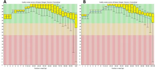
Both transcriptomic datasets presented in general good quality for all parameters tested. One of the most important parameters tested is the per base sequence content (Figure 3.1) that represents the quality scores (y-axis) per each position or some position range. The background of the graph is divided in three per base quality groups: very good (green); reasonable (orange); poor (red). The data showed good quality through the entire read, thus not requiring any read trimming
3.1.2.
Alignment
The genomes are full of repetitive sequences, and this can be a problem when we are mapping reads (Treangen et al., 2012). Since the goal of this work is to study pseudogenes with high similarity to the parental genes, we included only reads uniquely aligned. In both datasets the percentage of mapped read across the samples ranged between 80% and 90% (Table 3.1).
Other interesting result is that human dataset has an overall lower percentage of mapped reads when two hits are allowed. A higher percentage of uniquely mapped reads suggests that mouse genome has more repetitive regions than the human genome and that is concordant with other authors previous results (Haubold and Wiehe, 2006).
Figure 3.1.: Per base quality example plots (output from FastQC tool). (A) Mouse dataset, day 0, mates 1 (B) Human dataset, day0, replicate 2, mates 2.
17
Table 3.1.: Alignment summary for all samples of both datasets.
Data set Sample # Mapped Reads (max_hits=2) # Uniquely mapped Reads # Total Reads %Mapped Reads (max_hits=2) %Uniquely Mapped Reads
Mouse
Day0 92337051 83001177 101304040 91.1 81.9 Day1 88248264 78215517 96581066 91.4 81 Day2 97631234 86654482 107000680 91.2 81 Day3 90788837 82795456 98524424 92.1 84 Day4 88634463 81590842 95975150 92.4 85Hum
a
n
Day0_rep0 45859736 45282356 50481512 90.8 89.7 Day0_rep1 55063026 54397540 60463680 91.1 90 Day0_rep2 63598813 62787961 70484132 90.2 89.1 Day1_rep0 90493038 89071897 100526120 90 88.6 Day1_rep1 81649316 80442231 91587496 89.1 87.8 Day1_rep2 77550464 76388544 87427942 88.7 87.4 Day2_rep0 42776570 42203886 46882574 91.2 90 Day2_rep1 42681836 42106598 46922910 91 89.7 Day2_rep2 42563041 42042856 47695440 89.2 88.1 Day4_rep0 92074470 90744382 102437988 89.9 88.6 Day4_rep1 89022617 87745660 98885808 90 88.7 Day4_rep2 70518445 69535378 79234844 89 87.8 Day5_rep0 153534079 151319987 171841758 89.3 88.1 Day5_rep1 75743542 74659369 84068468 90.1 88.8 Day11_rep0 111273149 109583911 133940020 83.1 81.8 Day11_rep1 116764536 115093727 141720146 82.4 81.2 Day11_rep2 125656336 123755819 151379400 83 81.8 Day18_rep0 102438671 100960490 115552342 88.7 87.4 Day18_rep1 93981413 92591605 106219460 88.5 87.2 Day18_rep2 86559391 85301216 97691602 88.6 87.33.2.
Identification of New Pseudogenes
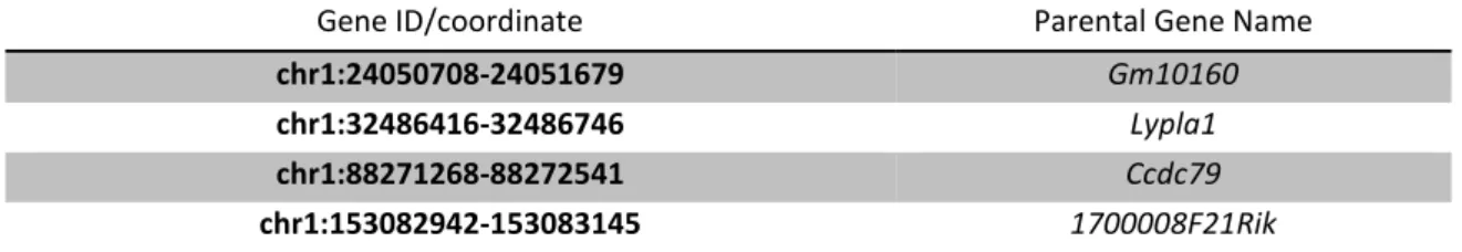
The workflow described to identify new pseudogenes (Section 2.3) was applied to mouse and human datasets. Analysis revealed 41 putative pseudogenes for mouse (Table 3.2) and 89 for human (Supplementary Table 1). The difference may be due to the higher number of samples in human dataset.
Table 3.2.: New putative pseudogenes discovered following the pipeline described at section 2.3 in mouse dataset.
Gene ID/coordinate Parental Gene Name
chr1:24050708-24051679 Gm10160
chr1:32486416-32486746 Lypla1
chr1:88271268-88272541 Ccdc79
18 chr11:3318094-3319118 Svop chr11:95864992-95865643 Gm10160 chr11:106994798-106995686 Timeless chr12:11239030-11239552 Gm11032 chr12:38868568-38869078 Gm10563 chr13:22835511-22837112 Zranb3 chr13:23325311-23326004 Cd59b chr13:100782127-100782952 Svop chr13:112881216-112882447 Snf8 chr15:33221975-33222671 Gm10491 chr15:76888487-76888750 Timeless chr15:99471290-99472055 Mybl2 chr16:13976683-13977868 Ifitm7 chr16:30955238-30955539 Sec14l4 chr16:38831711-38832823 Cd59b chr17:12895759-12896800 Arhgef40 chr17:32314259-32315309 Fance chr18:44735655-44735823 1700008F21Rik chr19:38950878-38951669 Gm10160 chr2:26639789-26639995 Bnc2 chr2:156993480-156994037 Limk2 chr2:177089204-177089784 Dpp6 chr3:88351639-88352590 Timeless chr3:123265980-123266769 Slc17a9 chr4:42716171-42717210 Gm13298 chr4:129727966-129728671 Letm1 chr4:140714527-140715809 Dlg1 chr4:152327691-152328501 Fance chr5:110772559-110773175 Amotl2 chr7:138889831-138890521 Gtdc1 chr8:12476765-12477829 Slc17a9 chr8:22174052-22174555 Atg13 chr8:105845572-105846232 Lman2l chr9:13843163-13843916 Zfp280d chr9:15315649-15316132 Letm1 chr9:57507830-57508505 Drosha chrX:52741373-52741588 Gm10491
Some putative pseudogenes possessed the same parental genes such as Timeless,
Gtdc1, Fance and Cd59b, so this result may be generated because of the repetitiveness
of specific sequences in genome that align these protein coding genes.
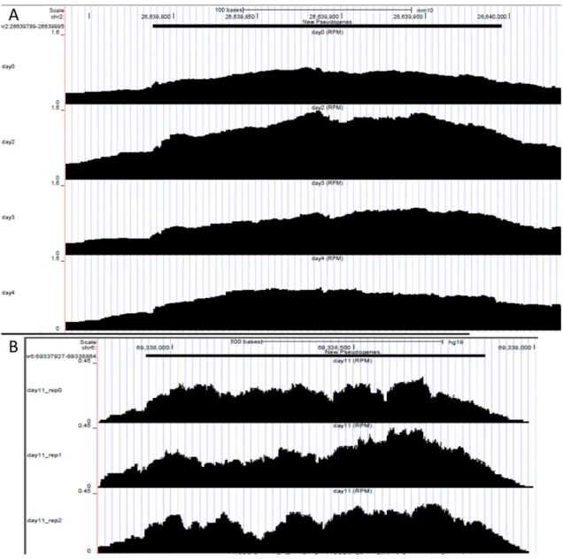
In Figure 3.2 it is possible to see the tracks in UCSC Genome Browser for two examples of new pseudogenes discovered in both datasets. Pseudogene annotation is represented at the bottom of each subfigure.
19
Figure 3.2.: UCSC Genome Browser tracks for new pseudogene examples. (A) Mouse new pseudogene in coordinates chr2:26639789-26639995 (parental gene – Bnc2; involved in regulation of transcription) in all time-points. (B) Human new pseudogene in coordinates chr6:69337927-69338864 (parental gene - REV3L; involved in DNA repair) in day 11, triplicate.
3.3.
Unsupervised Clustering Analysis
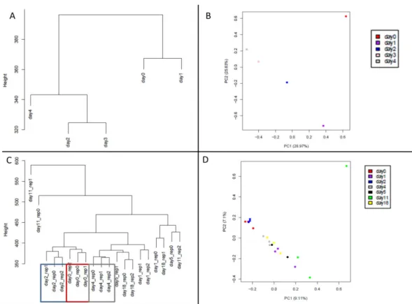
To characterize the pseudogene transcriptome we applied unsupervised methods, such as hierarchical clustering and PCA (Figure 3.3). They suggest that log(RPKM) values, in general, separated samples by time. In the case of human triplicate samples, they are clustered essentially according the time-point, with few exceptions. There are highlighted 3 examples (days 0, 2 and 4, Figure 3.3 C) where that is very clear. For mouse differentiation the two first PCs of pseudogene expression could explain half of the variance (54.6%), whereas for human data the percentage of variation decreased to 16.21%.
20
Figure 3.3.: Unsupervised clustering analysis of pseudogenes. (A) Clustering dendogram of mouse samples. (B) PCA plot of mouse samples. (C) Clustering dendogram of human samples. (D) PCA plot of human samples.
The same analysis was performed for protein coding genes, in order to assess the impact of the transcriptome in samples clustering. Both analyses revealed also time-series grouping (Figure 3.4), with a slight increase in the variance percentage represented by the two first PCs (60.25% for mouse and 18.44% for human).
Figure 3.4.: Unsupervised clustering analysis of protein coding genes. (A) Clustering dendogram of mouse samples. (B) PCA plot of mouse samples. (C) Clustering dendogram of human samples. (D) PCA plot of human samples.
21
This difference between the pseudogenes and protein-coding transcriptome can be explained by the overall lower and more variable expression of pseudogenes.
3.4.
Comparison of Statistic Methods for Differential
Expression Analysis
Differential expression analysis was performed using three different methods (EdgeR pairwise comparison, DESeq pairwise comparison and DESeq time-series analysis) in order to choose the best alternative for our study.
All methods show that differentially expressed genes (DEG) number increases along differentiation (Figure 3.5). DESeq pairwise comparison shows the lower number of DEG. DESeq time series analysis produces the high number of DEG. EdgeR pairwise comparison shows higher percentage of differentially expressed pseudogenes (DEP). One limitation of DESeq time series analysis is that this method does not provide a DEG list for each time point. This method only reports a p-value that indicates if a gene expression changes in any time, but not which time-point is that, despite retrieving fold-change for each time. We assessed that a gene was differentially expressed if have a p-value lower than 0.05 and an absolute logarithmic fold-change for that specific time-point higher than 0.58.
Figure 3.5: Gene expression analysis summarization for three distinct methods (DESeq pairwise comparison, DESeq time series analysis and EdgeR pairwise comparison). Numbers represents the number of differentially expressed genes (FDR or adjusted p-value < 0.05 and |log(Fc)|>0.58).
Only few DEP were consistently identified by all statistical (Figure 3.6), with higher number of common DEP found between the two DESeq pipelines. However, the DESeq-time workflow revealed to produce a higher number of DEP not found in any of
22
the other analyses. Although the low number of common pseudogenes, the two methods with the larger number of DEP (EdgeR pairwise comparison and DESeq time-series analysis), showed consistent expression fold-changes (Figure 3.7).
Figure 3.6.: Venn Diagrams for all time-points of differentially expressed protein coding genes and pseudogenes, between all methods.
Thus, these two methods differed essentially in the estimated p-values, where EdgeR package calculates a p-value for each pseudogene on each time-point and DESeq-time reports if a specific pseudogene expression varies over time. This do not allows us to make a certain decision about differential expression in specific time-points, so this is a reason why this analysis produces the highest number of DEP and differentially expressed protein coding genes. The DESeq-pairwise analysis appeared to be too strict, since it only identified a small number of DEP.
Figure 3.7.: Fold change comparison of differentially expressed pseudogenes between two different methods (EdgeR and DESeq time series analysis), for all time-points.
23
So, to obtain a confident reasonable amount of DEP for each time-point we performed the downstream differential expression analyses using the EdgeR method.
3.5.
Differential Expression Analysis and Pseudogene
Mappability
The differential expressed pseudogenes were determined comparing each time-point to initial stage with EdgeR method, using a false discovery rate (FDR) cut-off value of 0.05 and a absolute value of logarithmic fold change (log2) higher than
0.58.
To filter low covered or noisy pseudogenes in our samples, only those that present 60% of read coverage and appeared as differentially expressed for, at least, two time-points were considered for downstream analyses (Supplementary Table 2).
Comparison of volcano plots for both datasets revealed that the human differentiation showed higher amplitude of expression fold-changes (Figure 3.8 C). Due to the absence of replicates in mouse dataset, only pseudogenes with higher fold-changes were considered significant (Figure 3.8 A). Comparison of the fold-change with the mean expression level revealed that for mouse dataset, pseudogenes and protein-coding genes were equally distributed (Figure 3.8 B). In opposition, human pseudogenes showed lower mean expression levels but largest fold-changes (Figure
3.8 D). This was consistently observed for all time-points (data not shown).
Figure 3.8.: Day 1 expression view. Blue dots represent differentially expressed pseudogenes and red dots represent differentially expressed protein coding genes. (A) Volcano plot of mouse data. (B) MAplot of mouse data. (C) Volcano plot of human data. (D) MA plot of human data.
24
Figure 3.9 shows, for each dataset, an example of low read covered
pseudogenes. It may be due to the fact of pseudogenes have low uniqueness because they are very like their parental genes. To assess this hypothesis, the process was the one described in Section 2.8. To ensure the pseudogenes were being expressed and ot oise e e ui ed that at least 9 % of the appa le egio should o tai o e read aligned.
Figure 3.9.: UCSC Genome Browser example tracks for low covered DEP. (A) ENSMUSG00000083808 (mouse pseudogene), all days. (B) PGOHUM00000244028 (human pseudogene), day 0 triplicate and day 5 duplicate.
25
Only 20% of the DEP showed mappability higher than 90% (Table 3.3). We decided to apply this filter only after the statistical analysis, to not eliminate permanently candidate pseudogenes just because of their percentage of similarity with their cognates. Thus, although showing low mappability, these pseudogenes could be followed in the future using other experimental assays.
Table 3.3.: Troubleshooting summary.
3.6.
Pseudogenes and Neural Differentiation
When applying the statistical method we observed that the proportion of differentially expressed pseudogenes was very similar to the protein-coding genes. For three time-points (mouse data – days 1 and 2; human – day 18) the proportion of DEP was even higher than the number of differentially expressed protein-coding genes (Figure 3.10). These results may indicate the importance of pseudogenes in neural differentiation.
Figure 3.10.: Expression summary. Bar plots show the number of protein coding genes and pseudogenes differentially expressed. (A) Mouse data. (B) Human data.
Other interesting result is that day 11 of human data appears to have an abnormal expression of protein-coding genes and pseudogenes comparing to other time-points.
From all new pseudogenes discovered from mouse transcriptomic data, only one appeared as differentially expressed in mouse dataset at day 3 (chr9:57507830-57508505). Its parental gene was Drosha, involved in miRNA processing (Lee et al., 2003). The human transcriptomic dataset also revealed only one new differentially
Total number of pseudogenes Mappable> 90% #DEP Mappable > 90% ∩ DEP
Mouse 19444 18920 721 92