Growth and shared prosperity in Brazil

Texto

(1)Ensaios Econômicos Escola de Pós-Graduação em Economia da Fundação Getulio Vargas. N◦ 794. ISSN 0104-8910. Growth and shared prosperity in Brazil. Nanak Kakwani, Marcelo Neri, Fábio Vaz. Dezembro de 2017 URL: http://hdl.handle.net/10438/19458.

(2) Os artigos publicados são de inteira responsabilidade de seus autores. As opiniões neles emitidas não exprimem, necessariamente, o ponto de vista da Fundação Getulio Vargas.. ESCOLA DE PÓS-GRADUAÇÃO EM ECONOMIA Diretor Geral: Rubens Penha Cysne Vice-Diretor: Aloisio Araujo Diretor de Ensino: Caio Almeida Diretor de Pesquisa: Humberto Moreira Vice-Diretores de Graduação: André Arruda Villela & Luis Henrique Bertolino Braido. Kakwani, Nanak Growth and shared prosperity in Brazil/ Nanak Kakwani, Marcelo Neri, Fábio Vaz – Rio de Janeiro : FGV,EPGE, 2017 26p. - (Ensaios Econômicos; 794) Inclui bibliografia. CDD-330.

(3) Growth and Shared Prosperity in Brazil1 Nanak Kakwani University of New South Wales, NSW, Sydney, Australia Marcelo Neri FGV Social and FGV EPGE Fábio Vaz IPEA Abstract This paper proposes extensions of the idea of shared prosperity and inclusive development. It explores dynamic growth linkages between mean income, inequality and social welfare, on the one hand, and different labor ingredients and income sources, on the other. We propose a new decomposition method that quantifies the contributions to the shared growth patterns observed of social policies such as education, social security benefits, BPC and Bolsa Família and of classic labor market performance such as unemployment and participation rates, returns to schooling, hourly wages and hours worked. The paper also extends the idea of shared prosperity to shared opportunities that leads to new measures of inequity in opportunities. These can be calculated from household surveys that provide information on individuals’ access to various basic services in education, health, living conditions and so on. The proposed methodologies are applied to the Brazilian National Household Survey (PNAD) covering the period 2001-2013. Many policy questions relating to labor market performance and social policies are explored in explaining how Brazil achieved shared growth since the dawn of the new millennium. Keywords: 1. Inclusive Development; 2. Inequality; 3. Shared Prosperity; 4. Shared Growth; 5. Poverty Resumo Este artigo propõe extensões da ideia de prosperidade compartilhada e desenvolvimento inclusivo. Ele explora ligações tanto do nível como do crescimento entre renda média, desigualdade e bem-estar social, de um lado, e diferentes ingredientes trabalhistas e fontes de renda, por outro. Propomos um novo método de decomposição que quantifica as contribuições para os padrões de crescimento compartilhado observados de políticas sociais como educação, previdência social, BPC e Bolsa Família, e do desempenho no mercado de trabalho, medido pelo desemprego e taxas de participação, retornos da educação, salários por hora e horas trabalhadas. O artigo também estende a ideia de prosperidade compartilhada para a ideia de oportunidades compartilhadas que levam a novas medidas de desigualdade de oportunidades. Estas podem ser calculadas a partir de pesquisas domiciliares que fornecem informações sobre o acesso dos indivíduos a vários serviços básicos de educação, saúde, condições de vida e assim por diante. As metodologias propostas são aplicadas à Pesquisa Nacional por Amostra de Domicílios (PNAD) cobrindo o período de 2001 a 2013. Muitas questões políticas relacionadas ao desempenho do mercado de trabalho e políticas sociais são exploradas ao analisar como o Brasil alcançou um crescimento compartilhado desde o alvorecer do novo milênio até 2013. Palavras-chave: 1. Desenvolvimento Inclusivo; 2. Desigualdade; 3. Prosperidade Compartilhada; 4. Crescimento Compartilhado; 5. Pobreza. 1. A preliminary version of this paper was presented in the 42th Meeting of the Brazilian Economic Association held in Natal, Brazil during 2014. See https://www.anpec.org.br/encontro/2014/submissao/files_I/i12e54e711753a63e8ce47ab4deab7c6c13.pdf. 1.

(4) 1.. Introduction. Inclusive growth is a new development paradigm that has been widely discussed among governments, international organizations and other stakeholders in recent years. At this juncture, several countries in Asia are shifting their development goals from just poverty reduction toward other social objectives. For instance, India has focused on inclusive growth, while China has talked about creating a harmonious society. Similarly, Thailand has emphasized growth combined with equity. While it is unclear how these concepts precisely differ from one another, it is widely accepted that they are related to inclusive growth. Policy makers and experts have yet to formulate and agree on a single, cohesive definition of inclusive growth. Various organizations have in fact adopted their own definitions of inclusive growth. The Indian Planning Commission’s definition is the most comprehensive – defining inclusive growth as growth that alleviates poverty, generates employment, promotes equality of opportunities particularly in terms of access to health and education, fosters empowerment through formal schooling and skills development, encourages environmental sustainability, good governance and recognizes the role of women. With poverty reduction as the main social objective, the Indian Planning Commission’s definition expects inclusive growth to achieve many goals. Inequality reduction as a social objective is not covered in this definition but there is a concern for inequality of opportunities. Thus, this definition is a mixture of social objectives and policies that would achieve such objectives. The focus is on creating employment opportunities and empowerment through education and skill development. Under this definition, rapid economic growth is not seen as the key driver of poverty reduction. Meanwhile, the World Bank defines inclusive growth as growth that is sustained and broad based – reduces poverty and generates employment rather than merely supporting income redistribution. Like the Indian Planning Commission’s definition, the World Bank’s characterization of inclusive growth involves poverty reduction as the main social objective. The inclusiveness of growth hinges on the adoption of certain policies, particularly those geared toward creating productive employment to achieve poverty reduction. However, there are many other policies that can be implemented to reduce poverty. Thus, it may not be beneficial to restrict the policy space to only the generation of productive employment. There could be many poor who are not in the labor force such as elderly and disabled for whom the employment nexus is of little relevance. Furthermore, the focus on productive employment may result in a high level of unemployment among the poor, which may in turn increase poverty. World Bank has more recently proposed a new development model that focuses on the bottom 40% of the population. Under this new paradigm, it aims to: (i) lower extreme or absolute poverty in the world to 3% by 2030 and (ii) foster economic growth that benefits the bottom 40% of the population (Rosenblatt and McGavock, 2013). The second goal of targeting the bottom 40% of the population is built on the concept of shared prosperity. Growth fosters shared prosperity if the bottom 40% of the population could benefit from economic growth. The idea of shared prosperity appeals to various stakeholders because it has a well-defined but simple social welfare function. It is closely related to the notion of inclusive growth because it ensures that the bottom part of the population can participate in and benefit from growth. As a consequence the idea of shared prosperity is goal number 10 related with inequality within and between countries of the so-called Sustainable Development Goals (SDGs). 2.

(5) This paper proposes many extensions of shared prosperity that explore linkages between four dimensions: growth patterns, inequality, labor market performance and social policies. The paper demonstrates that the simple idea of shared prosperity is a powerful tool to answer many policy questions relating to labor market and social policies. The distinction is made between average prosperity (AP) and shared prosperity (SP), which are linked by an inequity component on top of the average prosperity measure. Thus following Kolm (1976a, 1976b), two measures of inequity are proposed: (i) relative or rightist measure of inequity and (ii) absolute or leftist measure of inequity. This study also develops a related idea of shared growth, which is measured by gain or loss in growth rate due to increasing (decreasing) equity in shared prosperity so the larger the gain, the greater the shared growth. The main methodological contribution of this paper is the new decomposition method that quantifies the contributions of social policies and labor market performance to the shared growth. The paper also extends the idea of shared prosperity to shared opportunities that leads to a new measure of inequity in opportunities. This new measure can be calculated from household surveys that provide information on individuals’ access to various basic services in education, health, living conditions and so on. The proposed methodologies are applied to the Brazilian National Household Survey (PNAD) covering the period 2001-2013. Many policy questions relating to labor market performance and social policies have been explored in explaining how Brazil achieved shared growth during past decade and continues the process in the new decade starting in 2011. The paper is organized as follows. Sections 2 and 3 propose simple indicators of shared prosperity in levels and in growth rates, respectively. Section 4 measures the contributions of mean income and inequality to share prosperity levels. Section 5 implements the same analysis of the previous section to understand the immediate determinants of shared growth dynamics. Section 6 sets the stage to understand the role played by different income sources in shared prosperity. In Section 7, the different income sources are considered in explaining the shared prosperity in Brazil. Section 8 calculates on a yearly basis the contributions of labor income and social policies such as social security benefits, BPC and Bolsa Família on shared growth and its immediate determinants. Section 9 digs one level further into the labor market determinants of shared growth. It incorporates classic labor market ingredients such as unemployment and participation rates, hours worked and hourly wages. Then the impacts on hourly wages of changes in education levels and their returns are measured, which may help to understand policies geared towards labor productivity growth in different parts of the income distribution. Section 10 proposes and applies a new measure of inequality of opportunities including productive employment, education attainment and school attendance. The last section provides the main conclusions of the paper.. 3.

(6) 2.. A Simple Indicator of Shared Prosperity. Suppose x is the income of an individual which is a random variable with density function f(x), then mean income of the population is defined as ∞. 𝜇 = ∫0 𝑥𝑓(𝑥)𝑑𝑥. (1). This is a simple measure of average standard of living enjoyed by the population. Although most economists focus on per capita GDP as a measure of country’s prosperity, it has many limitations in providing an adequate measure of people’s average welfare. In their book “Mis-Measuring our Lives: Why GDP Doesn’t Add up?”, Joseph Stiglitz, Amartya Sen and Jean-Paul Fitoussi (2010) have eloquently explained why GDP may provide a misleading measure of welfare. Given such limitations, the mean income defined in (1) can be suggested as a measure of average prosperity (AP) of the society. The World Bank is now promoting the idea of shared prosperity (SP), which is simply the mean of the bottom 40% of the population. More formally, suppose z is the income defined by 𝑧. 0.4 = ∫0 𝑓(𝑥)𝑑𝑥 then the shared prosperity indicator is defined by 𝑧. 𝜇𝑠 =. ∫0 𝑥𝑓(𝑥)𝑑𝑥. (2). 𝑧. ∫0 𝑓(𝑥)𝑑𝑥. which shows that the shared prosperity indicator is a weighted average of individual incomes. This is the welfare measure proposed by Basu (2001) that focuses on the bottom 20% of the population. World Bank’s new development model on the other hand focuses on the bottom 40% of the population. The idea of shared prosperity is based on the notion that a large proportion of the population should take part in and benefit from the growth process. The SP indicator is like other measures of social welfare defined over individual incomes such as Atkinson’s (1970) and Sen’s (1973), so it has an implicit inequality measure, which can be defined as 𝐼 =1−. 𝜇𝑠. (3). 𝜇. Then the SP indicator can be written as 𝜇𝑠 = 𝜇(1 − 𝐼). (4). which is a similar form of social welfare functions defined over the income space such as Atkinson’s and Sen’s indexes. Note that 𝐼 is not a usual measure of inequality such as the Gini index because it does not satisfy the weak transfer axiom. It will be referred to as a measure of inequity in shared prosperity and (1-𝐼) as a measure of equity in shared prosperity. 𝐼 is an mean independent measure of equity, which implies that the value of the measure remains unchanged if each income is altered by the same proportion. Such measures according to Kolm (1976a, 1976b) are called the relative or rightist measures of inequality. Alternatively, Kolm has proposed the absolute or leftists measures of inequality, which do not indicate any change in 4.

(7) inequality when each income is increased or decreased by the same amount. The absolute measure of inequity implicit in the SP social welfare function is defined as 𝐴 = 𝜇 − 𝜇𝑠. (5). The absolute inequity measure 𝐴 reflects the absolute differences in levels of living rather than relative differences.. 3.. Shared Growth. The idea of shared growth is now developed. To do so write (4) as 𝐿𝑛(𝜇𝑠 ) = 𝐿𝑛(𝜇) + 𝐿𝑛(1 − 𝐼) which on taking the first difference gives 𝛾∗ = 𝛾 + 𝑔. (6). where 𝛾 ∗ = ∆𝐿𝑛(𝜇𝑠 ) is the growth rate of shared prosperity, 𝛾 = ∆𝐿𝑛(𝜇) is the growth rate of average prosperity and 𝑔 = ∆𝐿𝑛(1 − 𝐼) is the growth rate of equity in shared prosperity, which will be positive (negative) if equity in shared prosperity is increasing (decreasing). Thus, there will be a gain (loss) in growth rate when equity is improving (deteriorating). For instance if 𝛾 ∗ =6% and 𝛾 =4%, it means that there is a gain of 2% in the growth rate of shared prosperity entirely attributed to the improvement of equity. The gain in growth rate signifies that economic growth is providing greater benefits to the bottom 40% population than the average gain to the society. This motivates the idea of shared growth, which can be measured by the gain in growth rate due to increasing equity in shared prosperity so that the larger the gain, the greater is the shared growth.. 4.. Patterns of Shared Prosperity in Brazil. This section provides trends in average and shared prosperity in Brazil from 2001 to 2013. The nationwide survey called PNAD is utilized in the empirical analysis. This is an annual survey conducted by the Brazilian Institute of Geography and Statistics (Instituto Brasileiro de Geografia e Estatística - IBGE) since 1967. Real per capita household income is used as individuals’ welfare measure. Real per capita income is defined as per capita nominal income adjusted for prices. The consumer price indexes corresponding to the PNAD survey periods are used to adjust for prices. Table 1 presents the estimates of average and shared prosperity in Brazil. Both AP and SP are measured in money metric (R$ per year in 2013 prices). The trends show that both AP and SP have been consistently increasing but the absolute gap between the two has also been widening. The trend growth rates presented in the last row of the table indicates that AP has been increasing at an annual rate of R$341 per person while SP has been increasing only at an annual rate of R$142 per person. In terms of absolute living standards, the bottom 40% of the population has thus performed worse than the average population; the gap between the two has been widening at an annual rate of R$199 per person. Absolute inequality, which is defined as the difference between AP and SP, has widened between 2001 and 2013. 5.

(8) The inequality measure developed in (3) is the relative measure of inequality. The trend depicted shows that relative inequality in Brazil has been declining from 79.5% in 2001 to 72.2% in 2013, representing a sharp decline of 0.63 percentage points annually. Thus, the relative gap in shared prosperity has been declining. This conclusion is also consistent with the declining Gini index in the same period. Absolute inequality measures reflect the absolute differences in levels of living rather than relative differences. In Brazil, absolute inequality is increasing but relative inequality is decreasing. This situation can be intuitively explained by the following illustration. Consider an economy composed of just two households with incomes $1,000 and $10,000. Suppose the poor household’s income is increased three fold while the rich household’s is scaled up two fold. Although relative inequality has decreased, the absolute difference in their incomes has sharply increased from $9,000 to $17,000. As such, relative inequality has decreased but absolute inequality has sharply risen. The concept of absolute inequity may have much intuitive appeal but in almost all debates on inequality the focus is always on the relative concept of inequality. In Brazil, the political debate on inequality is largely based on the Gini index, which is a relative measure of inequality. In layman’s language, the reference to the increasing gap between the rich and the poor may most likely mean the absolute difference between the rich and the poor. Which of the two concepts should be adopted to evaluate alternative policies? As Ravallion (2004) points, there is no economic theory that tells us that inequality is relative, not absolute. It is not that one concept is right and one is wrong but they are two different concepts. Table 1: Average and Share Prosperity in Brazil - R$ per year. Year 2001 2002 2003 2004 2005 2006 2007 2008 2009 2011 2012 2013 Trend 2001-20132. Table 1: Average and Share Prosperity in Brazil: R$ per year Average prosperity Shared prosperity Absolute inequality 7716.65 1580.56 6136.09 7724.84 1643.93 6080.91 7272.04 1577.39 5694.65 7514.04 1736.19 5777.85 7975.98 1870.09 6105.88 8724.18 2113.05 6611.13 8945.11 2197.81 6747.30 9372.73 2405.04 6967.69 9629,51 2480.57 7148.94 10235.07 2791.00 7444.07 11020.22 3067.77 7952.45 11405.06 3168.53 8236.53 341.11 142.02 199.09. Source: Author’s calculation. 2. Kakwani (1997) proposed the trend method used here.. 6. Relative Inequality 79.52 78.72 78.31 76.89 76.55 75.78 75.43 74.34 74.24 72.73 72.16 72.22 -0.63.

(9) 5.. Shared Growth in Brazil. Table 2 presents the annual growth rates of AP and SP. The growth trends presented show that growth rates of SP are higher than that of AP throughout 2001-2013. This implies that the bottom 40% of the population has performed consistently better than the average. The last column in Table 2 is obtained by subtracting the growth rates of AP from SP. The gains in growth rates measure the extent to which growth in mean income is shared. The larger is the gain the greater the shared growth. Substantial gains in growth rates are noticeable throughout the 2001-2013 period. The last row in Table 2 gives the trend growth rates in 2001-2013. AP has been increasing at an annual rate of 3.26% but the shared prosperity has been increasing at annual rate of 5.80%, resulting in an annual gain in growth rate of 2.54%. This growth pattern signifies an unprecedented reduction in inequality in the given period. Thus, average prosperity in Brazil has been increasing and more importantly the rate of this increase in prosperity has been much higher among the bottom 40% population. Thus, it can be unambiguously concluded that Brazil has sustained shared growth in the standard of living of its population. What are factors have contributed to Brazil’s success? This issue is explored in the next section. Table 2: Annual growth rates of Average and Shared Prosperity in Brazil - % Table 2: Annual growth rates of Average and Share Prosperity in Brazil Year AP SP Gain/Loss 2001 0.76 0.55 -0.20 2002 0.11 3.93 3.82 2003 -6.04 -4.13 1.91 2004 3.27 9.59 6.32 2005 5.97 7.43 1.46 2006 8.97 12.21 3.25 2007 2.50 3.93 1.43 2008 4.67 9.01 4.34 2009 2.70 3.09 0.39 2011 3.05 5.90 2.85 2012 7.39 9.46 2.06 2013 3.43 3.23 -0.20 Trend 2001-2013 3.26 5.80 2.54 Source: Author’s calculation. 6.. Determinants of Shared Prosperity. Brazil has been able to achieve an impressive improvement in both average and shared prosperity. In order to sustain this improvement, it is important to determine the factors that have contributed to this success. This section identifies these factors and measures the magnitudes of their impact on shared prosperity. Households generate income from many sources. Labor is the primary source of income generated by family members who are employed in the labor market. Who is employed in the family and how much income is generated by those employed is determined by a complex set of households’ demographic characteristics. In addition to labor income, households derive 7.

(10) income from other sources such as public and private transfers and financial assets, etc. This section measures the direct impact of these different factors that contribute to shared prosperity. Suppose households draw their income from k sources or there are k mutually exclusive income components and vi(x) is the income from the ith source of a household with total per capita income x such that 𝑥 = ∑𝑘𝑖=1 𝑣𝑖 (𝑥). (7). then the mean of the ith income source is given by ∞. 𝜇𝑖 = ∫0 𝑣𝑖 (𝑥)𝑓(𝑥)𝑑𝑥. (8). then substituting (7) into (8) gives 𝜇 = ∑𝑘𝑖=1 𝜇𝑖. (9). This equation can be used to estimate the contributions of each income source (component) to average prosperity. The term 100 × 𝜇𝑖 /𝜇 is the percent contribution of the ith income source to the total average prosperity. Similarly we can calculate the mean of the ith income source for the bottom 40% of the population: 𝑧. 𝜇𝑖𝑠 =. ∫0 𝑣𝑖 (𝑥)𝑓(𝑥)𝑑𝑥. (10). 𝑧. ∫0 𝑓(𝑥)𝑑𝑥. Substituting (7) into (10) gives 𝜇𝑠 = ∑𝑘𝑖=1 𝜇𝑖𝑠. (11). This equation provides the contribution of each income component to total shared prosperity. Thus, the term 100 × 𝜇𝑖𝑠 /𝜇𝑠 is the percent contribution of the ith income source to total shared prosperity. Policy making will benefit from determining which income sources contribute to shared prosperity and by how much. An income source can be said pro- shared-prosperity if it contributes more to the per capita income of the bottom 40% of the population than to the per capita income of the whole society. This motivates us to propose a new index: 𝜇 𝜇. 𝜑𝑖 = 𝜇𝑖𝑠𝜇. (12). 𝑠 𝑖. If 𝜑𝑖 is greater than 1, this implies that the ith income source contributes more to the per capita income of the bottom 40% population and thus 𝜑𝑖 will be called as the pro-shared prosperity index (PSPI). This index is like a targeting index informing how well a particular income source is targeted to the bottom 40% of the population. What are the sources of inequity in SP? To answer this question, we can use the following decompositions for the relative and absolute inequity:. 8.

(11) 𝐼 = ∑𝑘𝑖=1(𝜇𝑖 − 𝜇𝑖𝑠 )/𝜇. (13). and 𝐴 = ∑𝑘𝑖=1(𝜇𝑖 − 𝜇𝑖𝑠 ). (14). The term 100 × (𝜇𝑖 − 𝜇𝑖𝑠 )/𝜇 is the percent contribution of the ith income source to total relative inequity. Similarly, 100 × (𝜇𝑖 − 𝜇𝑖𝑠 ) is the percent contribution of the ith income to total absolute inequity. 7.. Determinants of Shared Prosperity in Brazil from 2001 to 2013. The following income sources are considered in explaining the shared prosperity in Brazil: a. Labor income b. Continuous Cash Benefit (Benefício de Prestação Continuada - BPC) c. Social Security d. Other incomes Labor income includes all earnings from occupation by all household members. A household’s labor income depends on two main factors: (i) number of household members who are employed and (ii) the level of earnings of working individuals. The next section provides a detailed discussion of the linkage between labor earnings and labor market characteristics. The BPC is an unconditional disability and old age grant targeted at the poor. It is a noncontributory social assistance program entirely comprised of a subsidy to the beneficiaries. Social security is the main component of social income in Brazil second only to labor earnings among all other sources collected by PNAD. The major portion of benefits is made of transfers that are to some degree linked with past contributions. Still the beneficiaries of social security do get public subsidies because the volume of transfers exceeds the volume of contributions. Other incomes include various types of non-social incomes to which the government does not make any contribution. They include private transfers from other families and non-government organizations, private pensions, rents and other earnings from assets such as interests and dividends. The income from the Bolsa Família Program (BFP) is also included in this income source3. Table 3 presents the percentage contributions of different income sources to total shared prosperity. Labor income is the most dominant factor shaping shared prosperity. In 2001, labor income alone contributed 79.23% to SP but declined to 72.75% in 2013. Thus, the contribution of labor income has been declining at an annual rate 0.51 percentage points. Meanwhile, the contribution of non-labor income has been increasing at an annual of 0.51 percentage points. The contribution of BPC has also increased but at a slower annual rate of 0.15 percentage points. The contribution of social security has remained stable at about 15%. While the contributions of social income have increased, non-social incomes have seen a declining trend in their contributions. 3. Due to technical problems to measure the incomes from the Bolsa Família Program (BFP) in the PNAD 2013, we did a separated analysis of its contribution to the Shared Prosperity in the period 2001-2012. The results, as well as the technical explanation, are in the two boxes (Box A and Box B) in the end of this section. In the present section, the income from the BFP is included in other incomes.. 9.

(12) Table 3: Contributions of income sources to total shared prosperity in Brazil – % Table 3: % contributions of income sources to total shared prosperity: Brazil Year Labor Social security BPC Other (incl. BFP) 2001 79.23 15.09 0.34 1.77 2002 78.30 14.91 0.55 2.48 2003 77.53 15.48 0.53 2.91 2004 75.98 14.02 1.44 5.15 2005 76.64 13.82 1.64 4.44 2006 74.83 13.37 2.18 6.26 2007 75.43 14.41 1.93 5.15 2008 75.90 13.44 1.83 5.80 2009 74.68 13.99 1.99 6.32 2011 73.22 15.52 1.83 7.09 2012 72.77 14.93 2.26 7.50 2013 72.75 15.16 2.24 7.46 Trend 2001-2013 -0.51 0.01 0.15 0.46 Source: Author’s calculation. As noted earlier, relative inequity in Brazil has been sharply declining over the 2001-2013 period. Total inequity in 2001 was 79.52% which declined to 72.22% in 2013, declining at an annual rate of 0.63 percentage points. Table 4 informs how contributions of various income sources contributed to the decline. The labor income has been the most dominant factor, which has contributed to an annual reduction of 0.36 percentage points. Social security has had relatively small impact on reducing inequity, only 0.04 percentage points annually in the period. Thus, the sharp reduction in relative inequity that has happened in Brazil has been contributed largely by labor and other incomes. Table 4: Contributions of income sources to inequity in shared prosperity - % Table 4: Contributions of income sources to total relative inequity in shared prosperity Year Per capita income Labor Social security BPC Other (incl. BFP) 2001 79.52 61.71 14.03 -0.01 0.49 2002 78.72 60.70 14.05 0.02 0.63 2003 78.31 59.84 15.13 -0.01 0.31 2004 76.89 58.77 14.90 0.01 0.07 2005 76.55 57.92 14.94 0.07 0.29 2006 75.78 57.78 14.75 0.08 0.04 2007 75.43 58.42 14.44 0.04 -0.19 2008 74.34 57.05 14.76 0.07 -0.24 2009 74.24 56.94 15.20 0.09 -0.54 2011 72.73 57.38 13.95 0.08 -0.59 2012 72.16 56.75 13.77 0.07 -0.38 2013 72.22 57.02 14.10 0.07 -0.82 Trend 2001-2013 -0.63 -0.36 -0.04 0.01 -0.11 Source: Author’s calculation. 10.

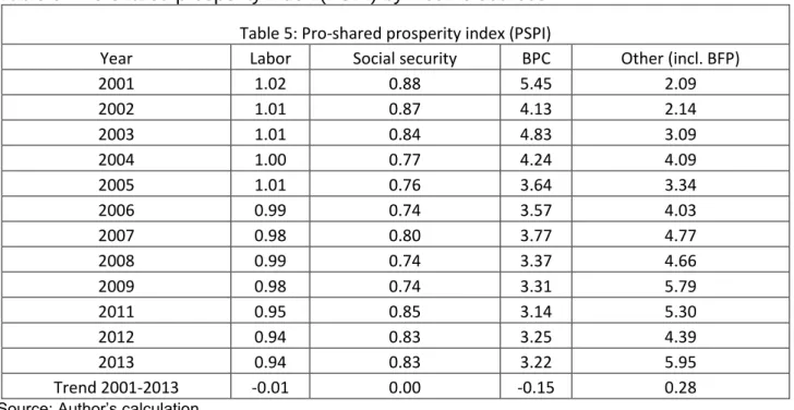
(13) As the data show, social programs do not have a large impact on inequality reduction, which is mainly due to the fact that their relative size is small compared to labor and other incomes. This does not imply that these programs are not well targeted. To measure their targeting efficiency, we can calculate their pro-shared prosperity index (PSPI) derived in (12). Table 5 presents the calculations of this index. The PSPI for the total income is 1, which is the bench mark. An index value greater than 1 implies that the particular income source benefits the bottom 40% more than the average. The larger is the value of the index, the greater the targeting efficiency. The PSPI for the labor income was 1.02 in 2001, which has declined to 0.94 in 2013. This implies that labor income is relatively becoming less well targeted at the bottom 40% of the population. The value of PSPI for the BPC has been over 3, which suggests that BPC supports shared prosperity. Social security, which has a large component of public subsidy, has been having the value of PSPI smaller than 1 over the recent period and thus cannot said to be well targeted. Table 5: Pro-shared prosperity index (PSPI) by income sources Year 2001 2002 2003 2004 2005 2006 2007 2008 2009 2011 2012 2013 Trend 2001-2013. Table 5: Pro-shared prosperity index (PSPI) Labor Social security BPC 1.02 0.88 5.45 1.01 0.87 4.13 1.01 0.84 4.83 1.00 0.77 4.24 1.01 0.76 3.64 0.99 0.74 3.57 0.98 0.80 3.77 0.99 0.74 3.37 0.98 0.74 3.31 0.95 0.85 3.14 0.94 0.83 3.25 0.94 0.83 3.22 -0.01 0.00 -0.15. Source: Author’s calculation. 11. Other (incl. BFP) 2.09 2.14 3.09 4.09 3.34 4.03 4.77 4.66 5.79 5.30 4.39 5.95 0.28.

(14) BOX A: Bolsa Família Program and Shared Prosperity – 2001 to 2012 Until 2003, Brazil had implemented four major cash transfer programs: (i) Bolsa Escola; (ii) Fome Zero; (iii) Bolsa Alimentação; and (iv) Vale Gás. Bolsa Escola is an income grant for primary education. Fome Zero and Bolsa Alimentação provide income grants related to food security while Vale Gás provides subsidies to help poor households buy cooking gas. Bolsa Família Program (BFP) took shape in 2003, early in the first term of Brazilian President Luiz Inácio Lula da Silva. It was established out of a merger of these four major cash transfer programs. It has now become a popular program benefiting more than 50 million people. The contribution of the Bolsa Família Program (BFP) to the total SP increased from 0.67% in 2001 to 7.08% in 2012 – indicating an annual increase of 0.52 percentage points. The increase in the contribution of the BFP to the SP in Brazil was the biggest among all income sources. The contribution of the BFP to the reduction in inequality was relatively small, mainly because it has a much smaller size than labor and other incomes, which does not imply that the program is not well targeted. The pro-shared prosperity index (PSPI) value for the BFP is around 8, the biggest among all income sources. This implies that it has been very effective in targeting the bottom 40% of the population and can be deemed as highly pro-shared prosperity. Table A.1: Contributions of income sources to total shared prosperity – % Year 2001 2002 2003 2004 2005 2006 2007 2008 2009 2011 2012 Trend 2001-2012. Labor BFP BPC 79.23 0.67 0.35 78.30 1.89 0.57 77.53 2.53 0.53 75.98 4.50 1.45 76.64 3.82 1.65 74.83 4.86 2.20 75.43 4.28 1.93 75.90 5.15 1.83 74.68 5.70 1.99 73.22 6.55 1.84 72.77 7.08 2.26 -0.53 0.52 0.16. S-security 15.09 14.91 15.48 14.02 13.82 13.37 14.41 13.44 13.99 15.52 14.93 -0.01. Other 4.66 4.32 3.93 4.04 4.06 4.74 3.95 3.67 3.65 2.87 2.97 -0.14. Source: Author’s calculation. Table A.2: Contributions of income sources to inequity in shared prosperity % Year 2001 2002 2003 2004 2005 2006 2007 2008 2009 2011 2012 Trend 2001-2012 Source: Author’s calculation. Labor 61.71 60.70 59.84 58.77 57.92 57.78 58.42 57.05 56.94 57.38 56.88 -0.40. BFP -0.06 -0.17 -0.23 -0.50 -0.44 -0.58 -0.55 -0.68 -0.77 -0.92 -0.97 -0.08. BPC S-security 0.01 14.03 0.57 14.05 0.01 15.13 0.02 14.90 0.32 14.94 0.12 14.75 0.04 14.44 0.08 14.76 0.09 15.20 0.09 13.95 12 0.07 13.73 -0.01 -0.03. Other 3.82 3.56 3.55 3.71 3.81 3.71 3.08 3.13 2.77 2.23 2.53 -0.14. Total 79.52 78.72 78.31 76.89 76.55 75.78 75.43 74.34 74.24 72.73 72.25 -0.66.

(15) BOX A: Bolsa Família Program and Shared Prosperity – 2001 to 2012 (cont.) Table A.3: Pro-shared prosperity index (PSPI) by income sources Year 2001 2002 2003 2004 2005 2006 2007 2008 2009 2011 2012 Trend 2001-2012. Labor 1.02 1.01 1.01 1.00 1.01 0.99 0.98 0.99 0.98 0.95 0.94 -0.01. BFP 8.38 7.97 8.03 8.34 8.32 8.15 8.59 7.96 8.15 7.52 7.09 -0.08. BPC 4.08 0.82 4.09 4.11 2.34 3.37 3.75 3.36 3.29 3.13 3.25 0.02. Source: Author’s calculation. 13. S-security 0.88 0.87 0.84 0.77 0.76 0.74 0.80 0.74 0.74 0.85 0.84 0.00. Other 0.97 0.96 0.89 0.87 0.85 0.98 0.98 0.90 0.98 0.95 0.88 0.00. Total 1.00 1.00 1.00 1.00 1.00 1.00 1.00 1.00 1.00 1.00 1.00 1.00.

(16) BOX B: Measuring the income from the Bolsa Família Program in the PNAD The PNAD survey does not contain specific questions that capture the household income derived from social programs like Bolsa Família, BPC, etc. Such information is collected in only one field that captures the income from "interest on savings accounts or other investments, dividends, social programs or other incomes". To separate the portion relating to Bolsa Família Program from other incomes, it is necessary to resort to the laws and design of the program to determine the so-called "typical values”. This process, however, is not free of errors, and the income obtained in this way should be considered only as a rough approximation of the actual income. In the case of Bolsa Família Program, the “typical values” have changed over time, as a result from increases in the benefit values and successive changes in the program design (Osorio and Souza, 2012). By 2011, the typical values depended only on the number of children aged 0-15 years, the number of young people aged 16-17 years (since December 2007) and if the family was in the range of extreme poverty. The set of combinations of values from the benefits was therefore finite. This allowed the separation of the incomes from the BFP until this year with a controllable error of measurement. From 2012, however, the typical values no longer exist because the design changes introduced by Decree No. 7,758/2012 and 7931/2013 created an extra benefit that covers the income gap relative to the poverty line for poor families, initially only for families with children under age six and later to all families in poverty. Exceptionally for PNAD 2012, an effort was made to separate the benefits of the BFP at the expense of a larger measurement error, since in 2012 the percentage of poor households who received the supplement income gap was still low (only families with children up to age six) and the "typical values" of the benefits were still valid to identify the household income from the BFP. From 2012, however, attempts to split the income of the BFP proved unviable.. 14.

(17) 8.. Determinants of Shared Growth Trends in Brazil. Based on the shared growth rates presented in Table 2, it can be concluded that Brazil has achieved a sustained shared growth in the standard of living of its population. What are the factors that have contributed to the shared growth in Brazil? This section attempts to shed light on this topic. Suppose 𝜇𝑡 is the AP in year t and 𝜇𝑖𝑡 is the mean of the ith income component in year t then based on (9) we have 𝜇𝑡 = ∑𝑘𝑖=1 𝜇𝑖𝑡. (15). Then it can be shown that 𝜇. 1. ∆𝐿𝑛(𝜇𝑡 )~ 2 ∑𝑘𝑖=1( 𝜇𝑖(𝑡−1) + (𝑡−1). 𝜇𝑖𝑡 𝜇𝑡. )∆𝐿𝑛(𝜇𝑖𝑡 ). (16). which shows that the growth rate of AP is the weighted average of the growth rates of individual income components - the weights being proportional to the average of income shares in each period. This equation informs the magnitude of contribution of each income component to the growth rate of AP. Similarly, we can explain the contribution of each income component to growth rate of SP using 1. 𝜇. ∆𝐿𝑛(𝜇𝑠𝑡 )~ 2 ∑𝑘𝑖=1( 𝜇𝑖𝑠(𝑡−1) + 𝑠(𝑡−1). 𝜇𝑖𝑠𝑡 𝜇𝑠𝑡. )∆𝐿𝑛(𝜇𝑖𝑡 ). (17). where 𝜇𝑠𝑡 is the SP in year t and 𝜇𝑖𝑡 is the mean of the ith component of the bottom 40% of the population in year t. This equation informs the magnitude of the contribution of each income component to the growth rate of SP. Shared growth is defined as the gain/loss in the growth rate of the SP, which is the difference between the growth rates of SP and AP. The difference of growth in (16) from (17) provides the contributions of each income component to shared growth. From Table 6, it is noted that the AP in Brazil has been increasing at an annual rate of 3.26% over the 2001-2013 period. The contribution of labor income is 2.47%, which means that the labor income has been the dominating factor in enhancing the AP in Brazil. The contribution of BPC is small at 0.09%. After the labor income, social security is the largest component contributing 0.68% to total growth in the AP. The SP has been growing at an annual rate of 5.80% leading to a gain of growth rate of 2.54%, which has resulted in shared growth in Brazil. Labor income contributing 1.40% to the gain in growth rate has been the major factor that has resulted in substantial shared growth in Brazil. The contribution of social security, which attracts substantial government subsidy, is 0.21%, which is relatively very small.. 15.

(18) Table 6: Contributions to trend growth rates in per capita income in Brazil 2001-2013 - % Table 6: Contributions to trend growth rates Brazil AP. SP. Gain/Loss. 2001-2013 Per capita income. 3.26. 5.80. 2.54. Labor. 2.47. 3.86. 1.40. Non labor. 0.79. 1.93. 1.15. Social security. 0.68. 0.88. 0.21. BPC. 0.09. 0.28. 0.19. Other (incl. BFP). 0.07. 0.82. 0.75. Source: Author’s calculation. 9.. The Role of Labor Market In Explaining Shared Growth. Brazil has been enjoying shared growth during the 2001-2013 period largely due to the income generated in the labor market. It is clearly important to determine the factors in labor market that have resulted in shared growth. PNAD provides labor force characteristics of individuals. The following variables, which have direct impact on the growth rate of labor income, have been identified. 1. Occupation rate: Employed persons as the share of labor force: e 2. Hours worked per employed persons: h 3. Labor force participation rate: Employed and unemployed persons as share of the population: l 4. Labor productivity: Labor income earned per hour of work: p=y/h The linkage between growth rate of per capita labor income and growth rates of the four labor force characteristics is provided through the following identity: 𝐿𝑛(𝑦) = 𝐿𝑛(𝑒) + 𝐿𝑛(ℎ) + 𝐿𝑛(𝑙) + 𝐿𝑛(𝑝) where y is the labor income per person. Using this identity, it is easy to show that the growth rate of per capita labor income is a sum of the growth rates of four labor force characteristics: 𝛾(𝑦) = 𝛾(𝑒) + 𝛾(ℎ) + 𝛾(𝑙) + 𝛾(𝑝). (18). The first factor is the occupation rate. Growth in occupation rate positively contributes to growth in per capita labor income. A similar interpretation is given to the other factors. Schooling is a major factor that influences productivity. It is generally true that the higher the level of schooling an individual possesses, the greater is his or her productivity. Thus, an increase in years of schooling should lead to an increase in productivity. However, the relationship between the two is not simple. Changes in years of schooling are also accompanied by changes in returns from schooling. The average hourly return of one year of schooling is given by 𝑟=. 𝑦 ℎ∗𝑆 16.

(19) where S is the mean years of schooling. Then growth in productivity p can be written as 𝛾(𝑝) = 𝛾(𝑟) + 𝛾(𝑆) which shows that growth rate in mean productivity can be decomposed into two components: the first component is the growth rate of average hourly rate of return from schooling and the second is the growth rate of average years of schooling. The growth of per capita labor income is equal to the growth rates of five components given by 𝛾(𝑦) = 𝛾(𝑒) + 𝛾(ℎ) + 𝛾(𝑙) + 𝛾(𝑆) + 𝛾(𝑟). (19). which provides a method of calculating the contributions of each of the five labor force characteristics to the growth rate of average labor income. This equation is derived for the whole population but a similar equation can be derived for the bottom 40% of the population as 𝛾(𝑦𝑠 ) = 𝛾(𝑒𝑠 ) + 𝛾(ℎ𝑠 ) + 𝛾(𝑙𝑠 ) + 𝛾(𝑆𝑠 ) + 𝛾(𝑟𝑠 ). (20). where 𝑦𝑠 , 𝑒𝑠 , ℎ𝑠 , 𝑙𝑠 , 𝑆𝑠 , and 𝑟𝑠 are per capita labor income, occupation rate, average hours of work, labor force participation rate, average years of schooling and average rate of return from schooling for the bottom 40% of the population, respectively. The shared growth in per capita labor income is given by 𝛾(𝑦𝑠 ) − 𝛾(𝑦) , which can be written as the sum of growth rates of five labor force characteristics: 𝛾(𝑦𝑠 ) − 𝛾(𝑦) = [𝛾(𝑒𝑠 ) − 𝛾(𝑒)] + [𝛾(ℎ𝑠 ) − 𝛾(ℎ)] + [𝛾(𝑙𝑠 ) − 𝛾(𝑙)] + [𝛾(𝑆𝑠 ) − 𝛾(𝑆)] + [𝛾(𝑟𝑠 ) − 𝛾(𝑟)] This equation quantifies the contributions of each of the labor force characteristics to the shared growth in the labor income. Table 7 presents the contributions of each of the labor force characteristics to the trend growth rates in per capita labor income. Labor income has been growing at an annual rate of 3.18% in 2001-2013. Of this trend growth rate, an increase in occupation has contributed 0.25% to AP – not very large but positive nonetheless. Labor force participation rate has also been increasing contributing 0.38% to the growth in labor income. The hours worked by employed persons have been decreasing, which has contributed to a decline in the growth rate of labor income by 0.39%. The declining hours of work may be due to the change in the nature of occupation, which is becoming more productive. It is the increase in hourly productivity that is contributing 2.93% to the growth in labor income. The growth in productivity is explained by two factors: (i) expansion of education and (ii) increase in the rate of return from each year of schooling. The completed years of schooling alone is contributing 2.23% to the growth in productivity. It is interesting to note that the expansion of education is accompanied by an increase in the average return per year of schooling, which has contributed 0.69% to the growth in total labor income. Labor income for the bottom 40% grew at an annual rate of 5.08%, which is predominantly explained by the productivity growth of 4.22%. Growth in productivity is explained by expansion of education and the increase in return from education. The completed years of schooling for the bottom 40% of the population increased at an annual rate of 4.22% and at the same time their 17.

(20) average rate of return from schooling increased at an annual rate of 1.38%. Thus, it can be concluded that the education has played the key role in the growth of the SP. The increase in rate of return from schooling might have been due to the real increases in the minimum wage in the 2001-2013 period but we cannot measure its direct impact. Table 7: Contributions of labor force characteristics to the trend growth of labor income: Brazil 2001-2013 -% Table 7: Contributions of labor force characteristics to the trend growth of labor income Labor force characteristics AP SP Gain/Loss 2001-2013 Employment rate 0.25 0.11 -0.15 Labor force participation rate 0.38 -0.19 -0.57 Hours worked per employed monthly Productivity hourly. -0.39 2.93. -0.44 5.60. -0.05 2.67. Per capita years of schooling. 2.23. 4.22. 1.98. Average hourly return per school year Per capita labor income. 0.69 3.18. 1.38 5.08. 0.69 1.90. Source: Author’s calculation. The last column in Table 7 provides the contributions of shared growth due to labor income. Occupation and labor force participation rates have negatively contributed to the shared growth. The shared growth has been largely contributed by the increase in productivity, expansion of education services and increasing returns from education. Table 8 provides the contributions of all factors to the total shared growth in per capita income. Total shared growth was 2.54% per annum - of which 1.47% is explained by the expansion of education and 0.51% by the increase in the rate of return from schooling. Contributions of BPC and social security are relatively small. Increases in occupation rate and labor force participation rates have a negative impact on shared growth. Table 8: Contributions of all factors to shared growth in per capita income - % Table 8: Contributions of all factors to shared growth in per capita income AP SP Gain/Loss 2001-2013 Employment rate 0.20 0.08 -0.11 LFPR 0.30 -0.14 -0.44 Hours worked -0.30 -0.33 -0.03 Productivity hourly 2.27 4.26 1.98 Years of schooling 1.73 3.21 1.47 Return from education 0.54 1.05 0.51 Labor 2.47 3.86 1.40 Non labor 0.79 1.93 1.15 Per capita income 3.26 5.80 2.54 Source: Author’s calculation. 10.. Shared Opportunities 18.

(21) Apart from expanding output, economic growth also creates opportunities in the economy that enhance well-being. For instance, growth generates employment, allowing people to earn income to be able to consume goods and services. However, these economic opportunities are not always equally shared by all. The poor generally benefit less from growth due to circumstances or market failures that prevent them from availing of these economic opportunities. Economic growth can directly create opportunities through market operations. More importantly, however, it generates resources in the form of tax revenues, fees, and fines, which governments use to create opportunities, particularly in education, health, housing, and so on. It is commonly perceived that governments can formulate policies and programs that facilitate the full participation of those who are less well off, ensuring that opportunities created by growth are equitably availed across the population. As such, governments play a key role in determining the pattern of growth that can result in equitable opportunities. Suppose o(x) is an opportunity enjoyed by a person with income x, then the average opportunity (AO) enjoyed by the society is given by ∞. 𝜗 = ∫0 𝑜(𝑥)𝑓(𝑥)𝑑𝑥 This is the average opportunity available, but does not inform how it is shared by the population. Similar to the idea of shared prosperity we can define shared opportunity (SO) as 𝑧. 𝜗𝑠 =. ∫0 𝑜(𝑥)𝑓(𝑥)𝑑𝑥 𝑧. ∫0 𝑓(𝑥)𝑑𝑥. which is the average opportunity enjoyed by the bottom 40% of the population. The inequity in opportunity can be defined as 𝐼𝑜 = 1 −. 𝜗𝑠 𝜗. Then the SO can be written as 𝜗𝑠 = 𝜗(1 − 𝐼𝑜 ) which is similar to Atkinson’s and Sen’s social welfare functions but defined over opportunity space. 𝐼𝑜 measures the proportional loss (or gain) in opportunity due to inequity (or equity) and therefore can be an indicator of inequity (equity) in opportunity. Note that unlike inequity measure 𝐼 defined in (3), which lies in the range 0 ≤ 𝐼 ≤ 1, this inequity measure 𝐼𝑜 lies in the rage −1 ≤ 𝐼𝑜 ≤ 1. The negative (positive) value implies that that opportunity is inequitable (equitable). 10.1. Occupation Opportunities. Labor income is generated through occupation in the economy. The people who do not have opportunity to be employed earn less income and enjoy a lower standard of living. Occupation itself has an intrinsic value. People who are employed enjoy greater satisfaction in life. Occupation rate is defined as the share of employed persons in the labor force. It informs whether or not those who are able and willing to work are able to obtain work. AO in occupation 19.

(22) is the occupation rate for the whole society and the SO in occupation is the average occupation rate for the bottom 40% of the population. Table 9 presents the empirical results for Brazil. The average occupation rate has increased from 90.50% in 2001 to 93.30% in 2013, resulting in an improvement in occupation rate at an annual rate of 0.28 percentage points. The occupation rate for the bottom 40% of the population is about 7 percentage points lower, which is also improving but at a slower annual rate of 0.15 percentage points. Thus, occupation opportunities are not equitable. The inequity index in occupation has increased from 5.88% in 2001 to 7.51% in 2013, with trend annual increase of 0.12 percentage points. The absolute gap in occupation rate between AO and SO has been widening. Table 9: Average and shared opportunity in occupation rate - % Table 9: Average and shared opportunity in employment rate Year Average prosperity Shared prosperity 2001 90.50 85.18 2002 90.73 85.67 2003 90.16 84.11 2004 90.88 85.26 2005 90.47 84.86 2006 91.39 85.63 2007 91.67 85.80 2008 92.70 87.36 2009 91.52 84.86 2011 93.08 86.42 2012 93.62 87.09 2013 93.30 86.30 Trend 2001-2013 0.28 0.15. Inequity 5.88 5.57 6.71 6.18 6.20 6.31 6.41 5.76 7.28 7.15 6.98 7.51 0.12. Source: Author’s calculation. 9.2. Productive Employment. International organizations such as the World Bank argue that the inclusiveness of growth hinges on poverty reduction policies particularly geared toward creating productive employment. Although productive employment generation has been widely discussed among governments, international organizations and other stakeholders in recent years, policies to create productive employment have yet to be clearly articulated. To ensure the generation of productive, Brazil has however developed a system of formal contracts, which provides considerable protection to employees, particularly those with low earnings. Still a large number of employees, especially those in the informal sector, do not enjoy the opportunity of securing a contractual employment. Large inequity still exists as seen in Table 10. The percentage of employees with formal contract has been low in Brazil at 61.14% in 2001, which increased to 72.02% in 2013; indicating an annual increase of 1.00 percentage points in the 2001-2013 period. In 2001, the bottom 40% of the population had only 38.05% of employees with formal contract indicating a high degree of inequity. Fortunately, inequity in contractual employment has been declining sharply at annual rate of 1.17 percentage points. In 2013, 54.30% of employees were working with formal contract among the bottom 40% of the population. The inequity index declined from 37.77% in 2001 to 24.60% in 2013. Thus, Brazil has made an 20.

(23) amazing progress in enhancing productive employment, which has been broad based with benefits going more to the poorest 40% of the population. Table 10: Employees with formal contract - % Table 10: Average and shared opportunity in employment with formal contract Year Average prosperity Shared prosperity 2001 61.14 38.05 2002 60.98 37.88 2003 62.24 39.03 2004 62.19 39.09 2005 62.99 40.50 2006 63.71 41.42 2007 65.14 43.35 2008 66.20 45.52 2009 66.83 45.49 2011 70.95 51.91 2012 71.25 52.27 2013 72.02 54.30 Trend 2001-2013 1.00 1.45. Inequity 37.77 37.89 37.30 37.14 35.70 34.99 33.45 31.24 31.93 26.83 26.63 24.60 -1.17. Source: Author’s calculation. 9.3. Opportunity in Education Attainment. An index of educational attainment of a family is defined as the average years of schooling of the occupied people in the household. It has been concluded earlier that this index of family education attainment makes large contribution to the household’s per capita labor income. Education is an opportunity everyone should enjoy. This section analyses the inequity in education attainment. The results are presented in Table 11. It is evident that education attainment in Brazil has been rapidly expanding. Completed years of schooling of the occupied people have on average increased from 6.64 years in 2001 to 8.68 years in 2013, resulting in an annual improvement of 0.17 years. Education attainment for the poorest 40% of the population was only 3.84 years in 2001 which indicated a large inequity of 42.14%. Fortunately, inequity has been declining at an annual rate of 1.26 percentage points. Although the improvement in education has contributed to large reduction in inequality in Brazil, the high inequity in education continues to exist. But Brazil has achieved commendable improvement in broadening its education which has benefited the bottom 40% of the population more than the average.. Table 11: Average and shared opportunity in education attainment - % 21.

(24) Table 11: Average and shared opportunity in education attainment Year Average prosperity Shared prosperity 2001 6.64 3.84 2002 6.82 4.05 2003 7.02 4.33 2004 7.21 4.54 2005 7.34 4.70 2006 7.57 4.96 2007 7.72 5.15 2008 7.93 5.45 2009 8.10 5.58 2011 8.35 5.89 2012 8.59 6.24 2013 8.68 6.37 Trend 2001-2013 0.17 0.21. Inequity 42.14 40.60 38.35 36.97 35.99 34.40 33.33 31.26 31.11 29.40 27.33 26.58 -1.26. Source: Author’s calculation. 9.4. School Attendance. Brazil’s conditional cash transfer programs are renowned worldwide given their twin objectives: (1) to alleviate poverty; and (2) to improve school attendance of children aged 5 years and older. The conditionality of the programs ensures that the children from the poor families acquire education so that poverty is not passed on to future generations. As these programs have been operating for quite some time, it is imperative to ask: how much inequity in school attendance does still exist? Empirical results presented in Table 12 provide the answer. In 2013, 98.50% of the children in the age group of 6-14 years old were regularly attending school. Only 1.50% of these children did not attend school, which may be due to illness or disability so that school systems cannot be held responsible for their non-attendance. Even among the bottom 40% of the population, 98.03% of the children in this age group attended school in 2013. The gap in school attendance has been narrowing and there is hardly any inequity in school attendance. The only conclusion that emerges is that Brazil offers opportunity to almost all children to attend school and get education. This is a commendable achievement. The conditional cash transfers may have been contributing to this outstanding success but there may have been other factors. Brazil’s education system may be providing quality education and inspiring teachers that may be motivating children to attend school.. Table 12: 6-14 years old children attending school - % 22.

(25) Year 2001 2002 2003 2004 2005 2006 2007 2008 2009 2011 2012 2013 Trend 2001-2013. Table 12: 6-14 years old children attending school Average prosperity Shared prosperity 95.33 93.33 95.81 94.14 96.11 94.60 96.30 94.79 96.70 95.55 97.09 95.96 97.14 96.20 97.55 96.79 97.65 96.97 98.31 97.87 98.28 97.79 98.50 98.03 0.26 0.39. Inequity 2.10 1.75 1.58 1.57 1.20 1.16 0.98 0.78 0.69 0.45 0.50 0.48 -0.14. Source: Author’s calculation. This section has presented an analysis of shared opportunity for selected components such as education and employment. However, the methodology developed here can be applied to a wide range of opportunities such as access to health services, water and sanitation, electricity, among others.. 23.

(26) 10. Conclusion In the recent years, inclusive growth is a new development paradigm that has been widely discussed among different stakeholders. The World Bank has proposed a new development model that focuses on the bottom 40% of the population. The idea is built on the concept of shared prosperity. Economic growth fosters shared prosperity if the bottom 40% of the population could participate in and benefit from it. Shared prosperity extensions proposed explore dynamic growth linkages between mean income, inequality and social welfare, on the one hand, and different labor ingredients and income sources, on the other. The paper demonstrates that the Idea of shared prosperity is a powerful tool to answer many policy related questions. The distinction is made between average prosperity (AP) and shared prosperity (SP), which are linked by inequity. The study also develops a related idea of shared growth, which is measured by gain (loss) in growth rate due to increasing (decreasing) equity in shared prosperity so the larger the gain, the greater the shared growth. We also propose a new decomposition method that quantifies the contributions to the shared growth patterns and its immediate determinants of social policies such as education, social security benefits, BPC and Bolsa Família and of classic labor market performance such as unemployment and participation rates, returns to schooling, hourly wages and hours worked. The methodologies are applied to the Brazilian National Household Survey (PNAD) covering the period 2001-2013. The main results are presented below: -. Growth trends of shared and average prosperity show that growth rates of SP are higher than that of AP throughout 2001-2013, which implies that the bottom 40% of the population has performed consistently better than the average. While AP has been increasing at an annual rate of 3.26%, SP has been increasing at an annual rate of 5.80%, resulting in an annual gain in growth rate of 2.54%.. -. Contribution of income sources to total shared prosperity: labor income is the most dominant factor shaping shared prosperity but its contribution has been declining at an annual rate of 0.51 percentage points in the 2001-13 period. The contribution of the Continuous Cash Benefit (BPC) has increased but at a slow rate of 0.15 percentage point, while the contribution of social security has remained stable.. -. Relative inequity in Brazil has been sharply declining over the 2001-2013 period. Once again, labor income has been the most dominant factor to this decline, contributing to an annual reduction of 0.63 percentage points. In contrast, BPC have contributed to reduction in inequity by only 0.01 annual percentage points. The sharp reduction in relative inequity has been contributed largely by labor income.. -. Labor income for the bottom 40% of the population grew at an annual rate of 5.08%, which is predominantly explained by the productivity growth of 5.60%. The completed years of schooling for the bottom 40% of the population increased at an annual rate of 4.22% and the average rate of return from schooling increased at 1.383% annually. Thus, it can be concluded that the education has played the key role in the growth of the SP. While occupation and labor force participation rates have negatively contributed to the shared growth, the last has been largely contributed by the increase in productivity, expansion of education services and increasing returns from education.. -. Total shared growth of per capita income was 5.80% per annum in 2001-2013, of which 3.21% is explained by the expansion of education and 1.05% by the increase in the rate of return from schooling. Contributions of BPC and social security are relatively small, 24.

(27) while increases in occupation rate and labor force participation rates have a negative impact in total shared growth. -. Shared Opportunities - The paper also extends the idea of shared prosperity to the one of shared opportunities that leads to a new measure of inequity in opportunities, calculated from household surveys that provide information on individuals’ access to basic services in education, productive employment, etc.. -. Occupation Opportunities: the average occupation rate has been increasing at an annual rate of 0.28 percentage points. The occupation rate for the bottom 40% of the population is also improving but at a slower annual rate of 0.15 percentage points. Thus, occupation opportunities are not equitable and are becoming less so.. -. Productive Employment: the percentage of employees with formal contract increased at the rate of 1.00 percentage points annually. Inequity in contractual employment has been sharply declining at an annual rate of 1.17 percentage points. Brazil has made an amazing progress in enhancing productive employment, which has been broad based with benefits going more to the poorest 40% of the population.. -. Opportunity in Education Attainment: completed years of schooling of the occupied people have on average increased an annual improvement of 0.17 years. Education attainment for the poorest 40% of the population was only 3.84 years in 2001, indicating large inequity of 42.14%. Fortunately, education attainment in the basis of the distribution had an annual increase of 0.21 year, reaching 6.37 years in 2013, which contributed to a decline in inequity at an annual rate of 1.26 percentage points, reaching 26.58% in 2013. High inequity in education continues to exist, but Brazil has broadened its education benefiting relatively more the bottom 40% of the population.. -. School Attendance: in 2013, even among the bottom 40% of the population, 98.03% of the children ageing 6-14 years old attended school. The gap in school attendance has been narrowing and there is hardly any inequity in school attendance for this age group, which is by itself a commendable achievement.. 25.

(28) References Atkinson, A.B. (1970) On the Measurement of Inequality, Journal of Economic Theory, Vol. 2, 244-263. Basu, Kaushik (2001). On the Goals of Development. In: Meier, G. M., & Stiglitz, J. E. (Eds.). Frontiers of development economics: the future in perspective. World Bank Publications. Campello, T.; Neri, M. (Org.). Programa Bolsa Família: uma década de inclusão e cidadania. Brasília: IPEA, 2013. 494 p. Kakwani N.; Neri, M.; Son, H. Linkages between pro-poor growth, social programme and the labor market: the recent Brazilian experience. World Development, vol 38, N.6, 2010 Kakwani, Nanak. Growth rates of per-capita income and aggregate welfare: An international comparison. Review of Economics and Statistics, v. 79, n. 2, p. 201-211, 1997. Kolm, S. C. (1976a). Unequal inequalities. I. Journal of Economic Theory,12(3), 416-442. Kolm, S. C. (1976b). Unequal inequalities. II. Journal of Economic Theory,13(1), 82-111. Osorio, R.; Souza, P.. O Bolsa Família depois do Brasil Carinhoso: uma análise do potencial de redução da pobreza extrema. (Nota Técnica nº 14). Ipea: Brasília, 2012. Ravallion, Martin (2004). Competing Concepts of Inequality in the Globalization Debate. In Ravallion, M., Thorbecke, E., & Pritchett, L. Brookings Trade Forum, pp. 1-38. Brookings Institution Press. Rosenblatt, David; McGavock, Tamara J. (2013). A Note on the Simple Algebra of the Shared Prosperity Indicator. World Bank, Washington, DC. Sen, A. (1973). On economic inequality. Clarendon Press, Oxford. Stiglitz, J. E., Sen, A., & Fitoussi, J. P. (2010). Mismeasuring our lives: Why GDP doesn't add up. The New Press.. 26.

(29)