MATERIAL AND METHODS Study Area

(1)

Engenharia Agrícola

ISSN: 1809-4430 (on-line) www.engenhariaagricola.org.br

Doi: http://dx.doi.org/10.1590/1809-4430-Eng.Agric.v38n5p705-717/2018

TEMPORAL DYNAMICS OF CLIMATOLOGICAL PARAMETERS AND HYDRIC BALANCE

IN THE MANAGEMENT OF AGRICULTURAL CROPS

Roberto Filgueiras

1*

_{, Vinicius M. R. de Oliveira}

2

_,

_{Fernando F. da Cunha}

2

_,

_{Everardo C. Mantovani}

2

1*_{Corresponding author. Universidade Federal de Viçosa (DEA/UFV)/ Viçosa - MG, Brasil. E-mail: roberto.f.filgueiras@ufv.br}

KEYWORDS

climate, geostatistical,

ordinary kriging,

thematic maps.

ABSTRACT

One of the main factors that determine the success of decision-making in the fields is the

climatic factor. This way, the geostatistical techniques have been used to represent and

understand the spatial or temporal dynamics of meteorological parameters. Therefore, the

aim of this research was to represent temporally through thematic maps, the average daily

behavior for meteorological variables and the hydric balance for the municipality of Patos

de Minas - MG. The climatic data were acquired from the automatic station INMET from

the years 1990 to 2015. Later, it was calculated the evapotranspiration and the hydric

balance for different capacities of available water in the soil (CAW): 24 mm, 48 mm, 80

mm and 112 mm. The climate variables showed temporal dependence, and through the

thematic maps, derived from the ordinary Kriging, it was possible to identify the seasons

of the year that are favorable for the production for the different crop groups.

INTRODUCTION

The climatic information, which are dynamic throughout the year, are relevant to the farmers, mainly, in the decision-making in the management of the plantations (Cecílio et al., 2012). The information about the averages of the climatic parameters allows a better understanding of the variability of these over the years, making the agricultural property planning to be executed with higher levels of accuracy, since the climatic variables exert a direct influence in the maximization of agricultural production (Moreno et al., 2016; Silva & Da Silva, 2016).

According to Martins et al. (2015), the climate knowledge is a key element to achieve a correct management of the agricultural crops, because through the knowledge of the climatic variables, it is possible to meet the evapotranspirometric demands. Highlighting the importance of the elements related to the climate and considering their importance in the management of rural properties, it is necessary that this information is available to the farmer in more understandable ways (Pereira et al., 2012). These elements are generally available in tables or graphs, so the interpretation is not direct, requiring a more careful analysis of them, since the temporal or spatial dependence of the data is not clearly represented in these forms.

In order to increase the efficiency of agricultural management and consequently to reduce losses that are directly related to adverse agrometeorological situations, the geostatistical techniques have been used to represent and understand the spatial or temporal dynamics of meteorological parameters (Sartori et al., 2010; Silva et al., 2010; Filgueiras et al., 2015; Emadi et al., 2016; Meyer et al., 2016; Reilly & Melillo, 2016; Gundogdu, 2017). The temporal and spatial behavior of these variables is analyzed by adjusting the experimental variogram to a theoretical variogram, since it is in this verification the dependence is observed over time and/or space (Isaaks & Srivastava, 1989; Heuvelink & Webster, 2001; Yamamoto & Landim, 2013).

(2)

Roberto Filgueiras, Vinicius M. R. de Oliveira, Fernando F. da Cunha, et al. 706

One way to solve this problem, and to make the execution of rural property planning more accurate, is to apply techniques based on geostatistical principles, such as ordinary kriging, known as the best linear unbiased estimator (Yamamoto & Landim, 2013). This can be considered, from geostatistical techniques, the most commonly used, based on the assumptions of the variable to be random and spatially correlated (Heuvelink & Webster, 2001).

Thus, the aim of this study was to represent, temporally, through thematic maps, the average daily behavior of climatological and hydric balance variables for the municipality of Patos de Minas-MG, aiming to make

available to the local farmer a product to assist in the decision-making, with regard to irrigation management.

MATERIAL AND METHODS

Study Area

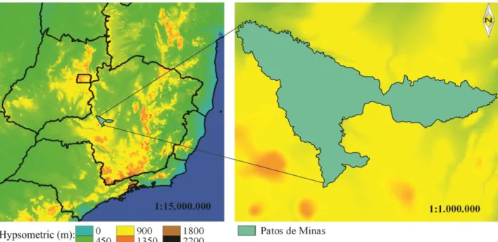
The study was carried out for the municipality of Patos de Minas, Minas Gerais (Figure 1), which is in the Alto Paranaíba mesoregion. It has diversified agriculture, with the production of corn, soybeans, beans, coffee, potatoes, garlic and carrots, besides having an extensive area with livestock farming (IBGE, 2015), being this region of great importance for Minas Gerais agriculture.

FIGURE 1. Location of the municipality of Patos de Minas in relation to the hypsometric map of the State of Minas Gerais.

The municipality of Patos de Minas-MG is located

between the pairs of coordinates 18° 15’27” south latitude,

45° 49’ 39.36” west longitude and 19° 00’ 46.44” south

latitude, 47° 00’ 18.36” west longitude (SIRGAS 2000

reference system) and average altitude of 832 m. The region has a predominant climate of Cwa type, of semi-humid tropical zone, with a minimum average temperature of 18ºC and an annual average of 22ºC or less. The climatic pattern is characterized by the presence of two well-defined seasons, one cold/dry, covering the months of April to September and the other warm/rainy, which extends from October to March. The average rainfall is 1600 mm year-1 (Alvares et al., 2013).

Acquisition of meteorological data

The meteorological information used in the study was taken from the INMET (National Meteorology Institute) historical database. The meteorological station present in the municipality has code 83531 and location in

the pair of coordinates 18°30’36” south latitude; 46°25’48”

west longitude (SIRGAS 2000 reference system).

The daily data taken from INMET for the station of interest were: rainfall (mm), maximum and minimum air temperature (°C), insolation (h), relative air humidity (%) and wind speed (U2) in the period from 1990 to 2015.

The period from 1990 to 2015 was selected because it did not contain any inconsistency of data. An analysis to verify if there were missing and discrepant data was carried out prior to their processing, following the methodology described by the World Meteorological Organization (OMM), suggested by Reboita et al. (2015). The discrepant data are values considered outliers for climatological variables in the region of interest, such as maximum monthly temperature of 60 °C (Reboita et al., 2015). In the absence of data occurrence, the average temperature and reference evapotranspiration (ETo) were calculated, the latter being calculated according to the Penman-Monteith equation, as recommended by FAO-56 (Allen et al., 1998).

Hydric Balance

The methodology proposed by Thornthwaite & Mather in 1955 was used to calculate the hydric balance (HB), as described by Vianello & Alves (2012). The daily average values of air temperature (°C) were used for the daily calculation of evapotranspiration. The rainfall data (mm) and evapotranspiration (mm) corresponding to a time series of 26 years were used to calculate the HB.

(3)

Temporal dynamics of climatological parameters and hydric balance in the management of agricultural crops 707

different CAW, different crop evapotranspiration (ETc) were considered. This approach with different CAW and ETc was proposed in order to simulate the water deficit for these different crops, where Kc values were based on Allen et al. (1998).

The ETc was calculated using the methodology (Equation 1) present in Bernardo et al. (2006).

ETc=ETo x Kc x Ks x Kl (1) that,

Ks - coefficient of irrigation frequency;

Kc - crop coefficient, and

Kl – coefficient of irrigation location, which is estimated by 0.1√P, where P is equal to PWA

(percentage of wet area) or PSA (Percentage of shaded area), with the highest value always prevailing between the two.

Thus, ETc, water deficit, excess and daily replenishment were calculated for the different agricultural crops, corresponding to an average of 26 years.

Geostatistical Analysis

After the calculation of the HB variables, the analysis of the data was carried out, in order to verify the possibility of the timing of the data through ordinary kriging.

Thus, the descriptive statistics of the data was analyzed, followed by the analysis of the temporal dependence of the data (Zimback, 2001; Sartori et al., 2010; Silva et al., 2010). After this analysis, which took place through the variogram, it was decided to carry out the geostatistical methodologies. The application of geostatistical techniques was used only in the occurrence of variographic amplitude, that is, when a range (t) was observed and then a stabilization of the variance of the data. If the premises of the geostatistics were not met, other interpolation methodologies would be applied, for example, the inverse of the distance square (Tayleur et al., 2016; Winter et al., 2016; Rodríguez-Amigo et al., 2017)

The dependence of the random variables over time was analyzed through [eq. (2)].

Y(t)=(_2N(t)1 ) ∑N(t)i=1 [Z(xi)-Z(xi+t)]² (2)

that,

(𝑡) - semivariogram for a vector t, days;

Z(x) and Z(x+t) - pairs of variables analyzed in the study, separated by a time interval, days,

N(t) - numbers of measured pairs.

The theoretical variograms model were adjusted to the experimental ones. Later, the Temporal Dependency Index (TDI) was calculated through the relation between the structural or temporal variance (C) and the baseline (C+ Co), through the [eq. (3)], proposed by Zimback (2001).

TDI=_C+CoC x100 (3)

It is considered a weak temporal dependence for values less than or equal to 25%, between 25 and 75%, moderate temporal dependence and for results greater than 75%, strong temporal dependence (Zimback, 2001). The quality of the model adjustments was verified through cross validation, which consists of comparing the observed values with those estimated by the models. After verifying the temporal dependence of the climatic variables, as well as the variables of the hydric balance, and adjusting the models, the interpolation was performed by the ordinary kriging method, aiming to represent the temporal distribution of the variables under study.

RESULTS AND DISCUSSION

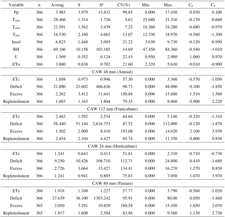
Table 1 shows the descriptive statistics of the daily averages, corresponding to 26 years of the following climatological variables: precipitation (Pp), maximum temperature (Tmax), medium temperature (Tmed), minimum temperature (Tmin), insolation (Insol), relative air humidity (RH), wind velocity (U2), reference evapotranspiration (ETo) and the daily averages corresponding to the variables of the hydric balance for the different values of CAW (crop evapotranspiration - ETc, Deficit, Excess and Replenishment).

(4)

TABLE 1. Descriptive statistics of the meteorological and hydric balance variables for the different CAW.

Variable n Averag S S² CV(%) Min. Max. Ca Ck

Pp 366 3.985 3.979 15.832 99,85 0.000 17.450 0.930 0.100

Tmax 366 28.466 1.314 1.726 4.62 25.680 31.310 -0.170 -0.660 Tmed 366 21.591 1.562 2.439 7.23 18.360 24.280 -0.680 -0.970 Tmin 366 16.530 2.160 4.665 13.07 12.330 18.970 -0.580 -1.300 Insol 366 6.823 1.448 2.095 21.22 3.630 9.730 -0.120 -0.990 RH 366 69.166 10.158 103.185 14.69 47.450 84.360 -0.540 -1.010

U 366 1.569 0.352 0.124 22.43 0.950 2.980 1.060 0.970

ETo 366 3.880 0.838 0.702 21.60 2.320 5.630 -0.010 -0.900 CAW 48 mm (Annual)

ETc 366 1.698 0.973 0.946 57.30 0.000 3.360 -0.570 -1.050 Deficit 366 21.880 21.602 466.636 98.73 0.000 48.000 0.100 -1.850 Excess 366 2.262 3.412 11.641 150.84 0.000 15.680 1.510 1.560 Replenishment 366 1.693 1.343 1.804 79.33 0.000 8.060 0.900 2.220

CAW 112 mm (Fruticulture)

ETc 366 2.463 1.592 2.534 64.64 0.000 5.140 -0.320 -1.310 Deficit 366 58.440 51.144 2,616.753 87.52 0.000 112.000 -0.120 -1.870 Excess 366 1.502 2.900 8.410 193.08 0.000 14.620 2.100 3.930 Replenishment 366 2.454 2.104 4.427 85.74 0.000 11.350 0.800 0.830

CAW 24 mm (Horticulture)

ETc 366 1.241 0.643 0.413 51.81 0.000 2.310 -0.710 -0.730 Deficit 366 9.250 10.426 108.710 112.71 0.000 24.000 0.410 -1.680 Excess 366 2.726 3.664 13.427 134.41 0.000 16.270 1.270 0.850 Replenishment 366 1.241 0.941 0.885 75.83 0.000 7.050 1.070 3.970

CAW 80 mm (Pasture)

ETc 366 1.918 1.108 1.227 57.77 0.000 3.790 -0.560 -1.020 Deficit 366 37.639 36.100 1303.242 95.91 0.000 80.00 0.050 -1.860 Excess 365 2.050 3.291 10.829 160.54 0.000 15.450 1.650 2.070 Replenishment 365 1.917 1.608 2.584 83.88 0.000 9.560 1.130 2.730 Pp: precipitation (mm); Tmax: maximum temperature (°C); Tmed: medium temperature (°C); Tmin: minimum temperature (°C); Insol: insolation

(h); RH: relative humidity (%); U2: wind speed (m s-1); ETo: reference evapotranspiration (mm); ETc: crop evapotranspiration (mm); n: number

of observations; s: standard deviation; S²: variance; CV: coefficient of variation (%); Ca: coefficient of asymmetry; Ck: coefficient of kurtosis.

The characteristics of the variograms models found for the climatological variables analyzed are shown in Table 2. For all the variables, the theoretical models that best represented the experimental variograms were the Gaussian models, followed by the Spherical model. The theoretical models were chosen because they presented a smaller error in the adjustment (Zimback, 2003). Jacomo et al. (2013) and

(5)

Temporal dynamics of climatological parameters and hydric balance in the management of agricultural crops

TABLE 2. The characteristics of the models found for the climatological variables.

Variable Variogram Model Co Co+C A r² TDI

Pp Spherical 0.330 16.650 6.580 0.955 0.980

Tmax Gaussian 0.001 1.821 3.204 0.709 0.999

Tmed Gaussian 0.001 2.591 3.932 0.705 1.000

Tmin Gaussian 0.010 4.939 4.399 0.749 0.998

Insol Spherical 0.001 2.185 5.750 0.889 1.000

RH Gaussian 0.100 109.100 4.780 0.898 0.999

U Spherical 0.006 0.138 5.400 0.894 0.958

ETo Gaussian 0.016 0.742 4.867 0.915 0.978

CAW 48 mm (Annual)

ETc Gaussian 0.001 1.001 3.775 0.737 0.999

Deficit Gaussian 1.00 497.000 4.832 0.853 0.998

Excess Spherical 2.190 12.470 8.230 0.968 0.824

Replenishment Spherical 0.221 1.764 3.960 0.797 0.875

CAW 112 mm (Fruticulture)

ETc Gaussian 0.001 2.676 4.156 0.798 1.000

CAW 24 mm (Horticulture)

ETc Gaussian 0.001 0.437 3.343 0.688 0.998

CAW 80 mm (Pasture)

ETc Gaussian 0.001 1.300 3.845 0.753 0.999

Pp: precipitation (mm); Tmax: maximum temperature (°C); Tmed: medium temperature (°C); Tmin: minimum temperature (°C); Insol: insolation

(h); RH: relative humidity (%); U: wind speed (m s-1_{); ETo: reference evapotranspiration (mm); ETc: crop evapotranspiration (mm); C}_o_{: nugget}

effect; Co + C: baseline; A: reach; r²: coefficient of multiple determination: TDI: time dependency index.

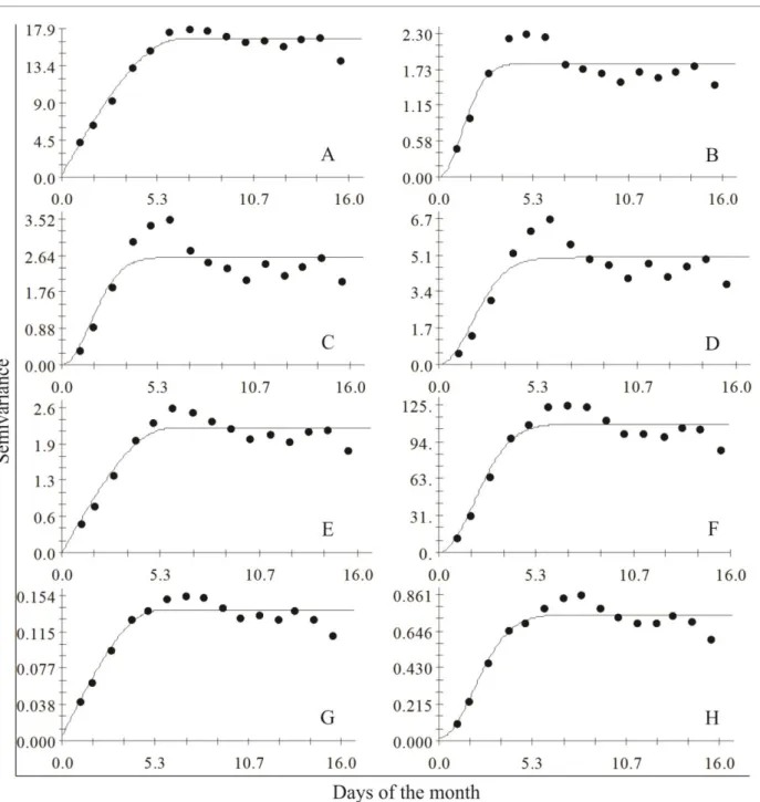
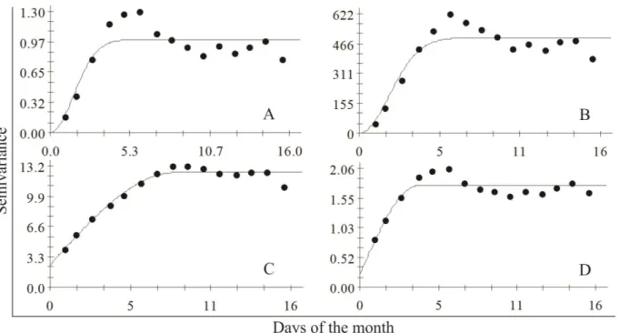
The Figures 2, 3, 4, 5 and 6 show the variographic analyzes of the climatological parameters and relative to the average daily hydric balance of 26 years. Table 2 shows that the variables presented temporal dependence. According to Zimback (2001), the only variable related to the hydric balance, which did not present a strong temporal dependence, was the estimated water excess for the CAW of 112 mm. Even so, this variable, according to the same author, showed moderate dependence.

(6)

Roberto Filgueiras, Vinicius M. R. de Oliveira, Fernando F. da Cunha, et al.

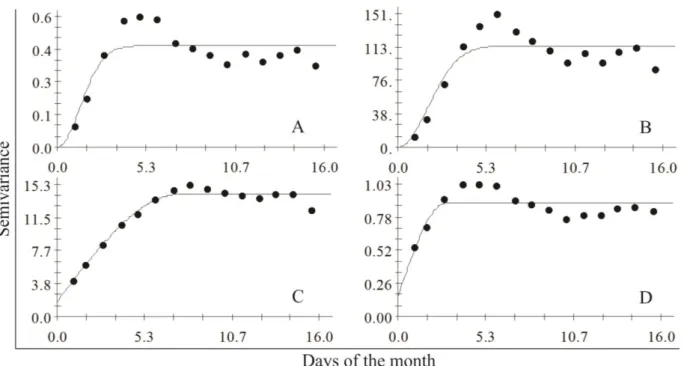
FIGURE 2. Isotropic Variogram of the annual daily average of the meteorological variables, precipitation (A), maximum temperature (B), medium temperature (C), minimum temperature (D), insolation (E), relative humidity wind velocity (G) and reference evapotranspiration (H).

On average, the meteorological variables presented a range (A) of 4.86 days. According to Yamamoto & Landim (2013), the range would be the distance at which the data reach a certain level, called baseline, and which is generally equal to the a priori variance of the data, or also, according to Sturaro (2015), the influence radius of a variable. In this way, becomes liable to statement that the climatological variables were correlated, on average, for approximately 5 days.

(7)

Temporal dynamics of climatological parameters and hydric balance in the management of agricultural crops

FIGURE 3. Isotropic Variograms of the annual daily average of reference evapotranspiration (A), hydric deficit (B), Excess (C) and Replenishment (D) estimated for the CAW of 48 mm.

(8)

Roberto Filgueiras, Vinicius M. R. de Oliveira, Fernando F. da Cunha, et al.

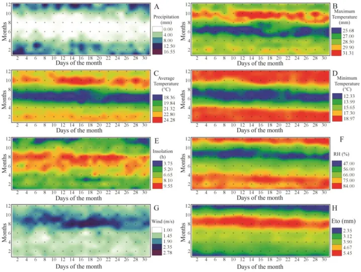
The average daily timing of the meteorological variables is shown in Figure 7, and the variability of the climatological parameters throughout the year (average of 26 years) can be observed in thematic maps, and in the abscissa (x) axis, the days of the month and, on the ordinate axis (y), the months of the year. The figure 7A shows that the lowest values of Pp occur in the months from June to August, with a predominance of low precipitation indexes during all the days of these months. However, the highest Pp values are clustered in the months from November to March, which was also observed by Alves & Rosa (2008)

in a study on the spatial data of the cerrado region in Minas Gerais and explained by Reboita et al. (2015).

(9)

83531, which corresponds to the same station used in this study. Reboita et al. (2015) did not find any discrepancy in the data series of the stations used, for precipitation and minimum and maximum temperature data.

The fact that the highest temperature values occur in the months of September and October does not imply that in other months high temperatures cannot occur, it only highlights the occurrence, more frequently, of the maximum temperatures during these months. The higher frequency of these, in the months of September and October, causes the predominance of the highest average temperatures in the same period, which can be observed by the reddish color throughout Figure 7C.

The predominance of the highest frequencies of minimum temperature (Figure 7D) occurs in the months from May to the beginning of August, verified by the bluish coloration of longitudinal occurrence in the minimum temperature thematic map, a fact also found in the study of Alves & Rosa (2008).The Figures 7E, 7F and 7G shows that the large amounts of hours of insolation associated with high wind speeds and low relative humidity are coupled to the range of maximum ETo values (Figure 7H), not neglecting the fact that high temperatures occur in this period (Figures 7B and 7C).

FIGURE 7. Average daily timing of meteorological data during the year.

Observing the timing, it is possible to identify months and days that, based on a long series of data, would be most likely to occur stresses to the cultivation of a certain crop, which can be water stress, temperature, insolation or even wind. In addition, this observation may be beneficial for planning pre-planting activities on the farm, such as soil preparation, acidity correction, pest and weed control. Another factor to be observed is the temperature requirement of some crops, such as pastures and forages,

temperatures below 15 ºC (Oliveira et al., 2014). In vegetables, such as garlic crop, require low temperatures, close to 14 ºC, for the bulbification process, and the production is compromised if it does not have this stimulation, caused by the low temperatures.

(10)

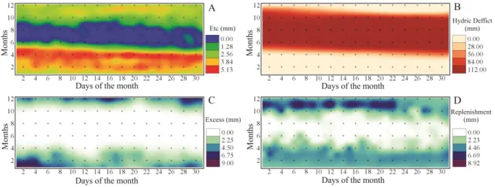
information is of great use to the farmers, since through the analysis of them, it is possible to know the exact moment in which each of these groups of crops needs hydric support. The management of the crop becomes more efficient, with information on how much and when the plant needs water, a fact that becomes easier, when it is precisely known, based on historical data, the production range of each crop group. According to Figure 8A, the highest ETc for annual crops in the municipality of Patos de Minas occur in the first

half of the year, with the highest values being concentrated in the months from February to April. This time, the crops with CAW of 48 mm are favored, as shown in Figures 8B, 8C and 8D. The most critical time for growing annual crops in this region is between May and October, since there is a water deficit during this period, with no water replenishment in the soil. The cultivation of annual crops at this time would only become viable with irrigation.

FIGURE 8. Annual daily average timing of hydric balance parameters for CAW of 48 mm, simulated value for annual crops (A - ETC, B - Deficit, C - Excess, D - Replenishment).

The highest evapotranspirometric (ETc) rates for fruit cultivation (Figure 9A), as well as for annual crops, tend to occur between February and May, but the fruit production has higher values than the annual crops. As the fruits are mostly perennial, they go through a long period of water deficit, which varies from May to the end of November, making irrigation support necessary to boost the production in those times.

FIGURE 9. Annual daily average timing of hydric balance parameters for CAW of 112 mm, simulated value for fruits (A - ETC, B - Deficit, C - Excess, D - Replenishment).

(11)

FIGURE 10. Annual daily average timing of the hydric balance parameters for CAW of 24 mm, simulated value for vegetables (A - ETC, B - Deficit, C - Excess, D - Replenishment).

The Pasture, in general, has the highest evapotransprometric demands concentrated in the month of April (Figures 11A). In the months from May to the end of October, the soil for these crops is under water deficit, which makes irrigation essential for biomass production at that time (Figure 11B), since during this period the soil presents small levels of the replenishment, so the available water capacity for these crops is not supplied (Figure 10C, D).

FIGURE 11. Annual daily average timing of the hydric balance parameters for CAW of 80 mm, simulated value for pasture (A - ETC, B - Deficit, C - Excess, D - Replenishment).

(12)

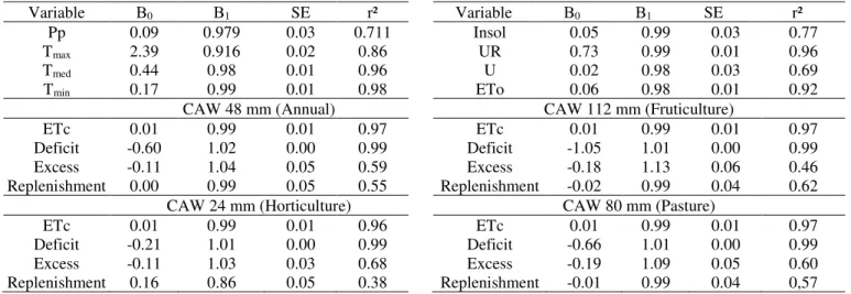
TABLE 3. Parameters of the cross-validation of the meteorological variables and the hydric balance.

Variable Β0 Β1 SE r² Variable Β0 Β1 SE r²

Pp 0.09 0.979 0.03 0.711 Insol 0.05 0.99 0.03 0.77

Tmax 2.39 0.916 0.02 0.86 UR 0.73 0.99 0.01 0.96

Tmed 0.44 0.98 0.01 0.96 U 0.02 0.98 0.03 0.69

Tmin 0.17 0.99 0.01 0.98 ETo 0.06 0.98 0.01 0.92

CAW 48 mm (Annual) CAW 112 mm (Fruticulture)

ETc 0.01 0.99 0.01 0.97 ETc 0.01 0.99 0.01 0.97

Deficit -0.60 1.02 0.00 0.99 Deficit -1.05 1.01 0.00 0.99

Excess -0.11 1.04 0.05 0.59 Excess -0.18 1.13 0.06 0.46

Replenishment 0.00 0.99 0.05 0.55 Replenishment -0.02 0.99 0.04 0.62

CAW 24 mm (Horticulture) CAW 80 mm (Pasture)

ETc 0.01 0.99 0.01 0.96 ETc 0.01 0.99 0.01 0.97

Deficit -0.21 1.01 0.00 0.99 Deficit -0.66 1.01 0.00 0.99

Excess -0.11 1.03 0.03 0.68 Excess -0.19 1.09 0.05 0.60

Replenishment 0.16 0.86 0.05 0.38 Replenishment -0.01 0.99 0.04 0,57 Β0 - intercept; Β1– coefficient of regression; SE - Standard error; r2 - coefficient of determination.

The analysis of the variables of the cross-validation allows to verify that the theoretical models adjusts well to the experimental ones, since the B0 and SE approached zero in all the variables and the B1 and r² approached of the unit in the majority of the parameters studied. The only variables that did not present a high coefficient of determination, of the cross validation, were excess and replenishment, being verified this fact in all variables studied.

CONCLUSIONS

The climatic variables, as well as the variables of the hydric balance, presented temporal dependence, making possible the execution of the geostatistical methodology used in the study. Through the thematic maps, derived from ordinary kriging, it was possible to identify the favorable production seasons for the different crop groups analyzed, as well as to make it possible to plan, with the highest level of accuracy, planting times for this region, as well as the need for irrigation in the critical moments of the crops.

From this methodology, it is easy to interpret the behavior of the climatological variables, as well as the dynamics of the hydric balance throughout the year, for the different crop groups, making the decision-making easier for the farmers of the region.

It is important to emphasize that this methodology can be replicated in other regions, in order to simplify the interpretation of the information, both climatological and relative to the hydric balance for the different crops of interest.

ACKNOWLEDGMENTS

We would like to thank the financial support (PhD scholarship) given by CNPq (Conselho Nacional de Desenvolvimento Científico e Tecnológico) and CAPES (Coordenação de Aperfeiçoamento de Pessoal de Nível Superior) to the first author and second author, respectively.

REFERENCES

Allen RG, Pereira LS, Raes D, Smith M (1998) FAO Irrigation and drainage. Food and Agriculture Organization of the United Nations 56(97):e156.

Alvares CA, Stape JL, Sentelhas PC, De Moraes G, Leonardo J, Sparovek G (2013) Köppen’s climate

classification map for Brazil. Meteorologische Zeitschrift 22(6):711-728.

Alves AKA, Rosa RR (2008) Espacialização de dados climáticos do Cerrado mineiro. Horizonte Científico 2(1). Available in:

http://www.seer.ufu.br/index.php/horizontecientifico/articl e/view/3990

Bernardo S, Soares AA, Mantovani EC (2006) Manual de irrigação. Viçosa, Ed. UFV, 625p.

Cecílio RA, Silva KR, Xavier AC, Pezzopane JRM (2012) Método para a espacialização dos elementos do balanço hídrico climatológico. Pesquisa Agropecuária Brasileira 47(4):478-488.

Emadi M, Shahriari AR, Sadegh-Zadeh F, Jalili Seh-Bardan B, Dindarlou A (2016) Geostatistics-based spatial distribution of soil moisture and temperature regime classes in Mazandaran province, northern Iran. Archives of Agronomy and Soil Science 62(4):502-522.

Filgueiras R, Nicolete DAP, Carvalho TM, Cunha AR, Zimback CRL (2015) Distribuição temporal das variáveis climatológicas em Botucatu-SP. Faculdade de Ciências Agrárias e Veterinárias, Universidade Estadual Paulista. DOI: https://doi.org/10.12702/IV-SGEA-a46

Gundogdu IB (2017) Usage of multivariate geostatistics in interpolation processes for meteorological precipitation maps. Theoretical and Applied Climatology 127(1– 2):81-86.

Heuvelink G, Webster R (2001) Modelling soil variation: past, present, and future. Geoderma 100(3):269-301.

IBGE - Instituto Brasileiro de Geografia e Estatística (2015) Zoneamento Agrícola. IBGE, 50p.

(13)

Jacomo CA, Tachibana VM, Flores EF (2013)

Geoestatística espaço-temporal e cluster para classificação de dados de precipitação anual do oeste paulista. In: Simpósio de Geoestatística Aplicada em Ciências Agrárias. Botucatu, Faculdade de Ciências Agronômicas, Anais...

Martins E, Oliveira Aparecido LE, Santos LPS, De Mendonça JMA, De Souza PS (2015) Influencia das condições climáticas na produtividade e qualidade do cafeeiro produzido na região do Sul de Minas Gerais. Coffee Science 10(4):499-506.

Meyer S, Blaschek M, Duttmann R, Ludwig R (2016) Improved hydrological model parametrization for climate change impact assessment under data scarcity-The potential of field monitoring techniques and geostatistics. Science of The Total Environment 543(Part B):906-923. Moreno NB, Silva AA, Silva DF (2016) Análise de Variáveis Meteorológicas para Indicação de Áreas Agrícolas Aptas para Banana e Caju no Estado do Ceará (Analysis of meteorological variables for indication of agricultural areas). Revista Brasileira de Geografia Física 9(1):1-15.

Oliveira VMR, Drumond LCD, Silva LOD, Gentil FH (2014) Produção de Tifton-85 irrigado submetido a doses de adubação nitrogenada no primeiro ano de implantação. Enciclopédia Biosfera 10(19):1563-1572.

Pereira MDB, Souza Filho JF, Moura MO (2012) Análise da pluviosidade na microrregião de sapé, paraíba e sua relação com a produção da cana-de-açúcar. Revista Geonorte 3(9):910-921.

Perin EB, Novaes VLF, Da Silva, Ricce W, Massignam AM, Pandolfo C (2015) Interpolação das variáveis climáticas temperatura do ar e precipitação: revisão dos métodos mais eficientes. Geografia 40(2):269-289. Reboita MS, Rodrigues M, Silva LF, Alves MA (2015) Aspectos climáticos do estado de minas gerais (climate aspects in minas gerais state). Revista Brasileira de Climatologia, 17. Available in:

http://revistas.ufpr.br/revistaabclima/article/view/41493 Reilly J, Melillo J (2016) Climate and Land: tradeoffs and opportunities. Geoinfor Geostat: An Overview 4(1-2):5672-5679.

Rodríguez-Amigo MC, Díez-Mediavilla M, González-Peña D, Pérez-Burgos A, Alonso-Tristán C (2017) Mathematical interpolation methods for spatial estimation of global horizontal irradiation in Castilla-León, Spain: A case study. Solar Energy 151(1):14-21.

https://doi.org/10.1016/j.solener.2017.05.024 Sartori AAC, Silva AF, Ramos CMC, Zimback CRL (2010) Variabilidade temporal e mapeamento dos dados climáticos de Botucatu-SP. Irriga 15(2):131-139.

Silva AF, Zimback CRL, Oliveira RB (2010) Cokrigagem na estimativa da evapotranspiração em Campinas, SP. Tekhne e Logos 2(1)16-29.

Silva G, Da Silva DF (2016) Análise da Influência Climática Sobre a Produção Agrícola no Semiárido Cearense (Analysis of Climate Influence on Agricultural Production in Semiarid Cearense). Revista Brasileira de Geografia Física 9(2):643-657.

Sturaro JR (2015) Apostila de geoestatistica básica, Rio Claro, UNESP, IGCE, 34p.

Tayleur CM, Devictor V, Gaüzère P, Jonzén N, Smith HG, Lindström Å (2016) Regional variation in climate change winners and losers highlights the rapid loss of cold-dwelling species. Diversity and Distributions 22(4):468-480. https://doi.org/10.1111/ddi.12412

Vianello RL, Alves AR (2012) Meteorologia básica e aplicada. Viçosa, Imprensa Universitária-Universidade Federal de Viçosa, 460p

Winter JM, Beckage B, Bucini G, Horton RM, Clemins PJ (2016) Development and Evaluation of High-Resolution Climate Simulations over the Mountainous Northeastern United States. Journal of Hydrometeorology 17(3):881-896. https://doi.org/10.1175/JHM-D-15-0052.1 Yamamoto JK, Landim PMB (2013) Geoestatística: conceitos e aplicações. Oficina de Textos.