© The Author(s) 2011. This article is published with open access at Springerlink.com csb.scichina.com www.springer.com/scp
*Corresponding author (email: [email protected]) SPECIAL TOPICS:
Statistical Physics and Mathematics for Complex Systems December 2011 Vol.56 No.34: 37073716 doi: 10.1007/s11434-011-4755-x
Globalization and long-run co-movements in the stock market for
the G7: An application of VECM under structural breaks
MENEZES Rui
1,2*& DIONÍSIO Andreia
3,4 1ISCTE-IUL Business School, Av das Forças Armadas, 1649-026 Lisboa, Portugal;
2 UNIDE-IUL Research Center, Av das Forças Armadas, 1649-026 Lisboa, Portugal; 3 University of Évora, Largo dos Colegiais 2, 7000-803 Évora, Portugal;
4 CEFAGE-UE Research Center, Largo dos Colegiais 2, 7000-803 Évora, Portugal
Received May 17, 2011; accepted June 27, 2011
This paper analyzes the process of long-run co-movements and stock market globalization on the basis of cointegration tests and vector error correction (VEC) models. The cointegration tests used here allow for structural breaks to be explicitly modeled and breakpoints to be computed on a relative-time basis. The data used in our empirical analysis were drawn from Datastream and comprise the natural logarithms of relative stock market indexes since 1973 for the G7 countries. The main results point to the conclusion that significant causal cointegration effects occur in this context and that there is a long-run relationship that governs the worldwide process of market integration. Globalization, however, is a complex adjustment process and in many cases there is only evidence of weak market integration which means that non-proportional price transmission occurs in the market along with proportional changes. The worldwide markets, as expected, appear to be driven in general by the US stock market.
globalization, long-run co-movements, market integration, VECM, cointegration, structural breaks
Citation: Menezes R, Dionísio A. Globalization and long-run co-movements in the stock market for the G7: An application of VECM under structural breaks.
Chinese Sci Bull, 2011, 56: 37073716, doi: 10.1007/s11434-011-4755-x
Recent debates on long-run co-movements and economic globalization have led to extensive research that try to de-termine its causes and explain the consequences of these phenomena in terms of market performance and their ability to adjust globally to economic boosts and crises. This has been relevant in the case of financial markets and in partic-ular in stock market studies [1–9]. However, many of these studies lack a theoretical background of what is globaliza-tion and how it can be measured, and rely solely on conclu-sions based on correlation relationships among stock re-turns.
Although returns are considered the most important fac-tor affecting invesfac-tor decisions, prices may also play a role in the process of market adjustment and, in particular, in the process of market integration. In fact, while traditionally returns are considered as a complete and scale-free
sum-mary of investment opportunities and have more attractive statistical properties (e.g. stationarity and ergodicity) than prices, the latter incorporate important information about the long-run characteristics of the market that are, by con-struction, lost in the former. Indeed, continuous compound-ing returns (rt) are typically computed as the log ratio
be-tween prices (Pt) at dates t and t1, that is, rt = (logPt) and
by taking the first difference of the observed variable Pt one
removes the long-run information contained in the data. Besides, the current econometric technology allows us to deal with the problem of nonstationarity of prices over time in a fairly trivial way using the concept of cointegration. And, even the problem of scaling can be easily overcome by relative prices rather than the originally observed stock prices or indexes without any loss of generality.
Under these circumstances, we argue that in order to keep the model as general and flexible as possible, re-searchers should keep as much original information as
pos-sible to avoid data manipulation distortions, and to allow for long- and short-run effects to work together in order to make meaningful predictions. Why should one discard the long-run information contained in the data when its econo-metric treatment is nowadays standard methodology?
Without the long-run information, any study on globali-zation and market integration based on price movements becomes virtually impossible to perform. The idea is that long-run movements of log prices highlight the equilibrium1) relationships between the data, whereas short-run move-ments of returns or log price changes capture deviations to the equilibrium relationships that also adjust in the short-run. It is possible that two data series move together in the short-run while they diverge in their long-run movements, a situation where price data do not cointegrate despite returns or price changes display significant relationships.
Long-run and short-run price movements can be modeled by an error correction framework. One advantage of the error correction model is that it allows for historical prices and returns to affect simultaneously but separately the be-havior of current stock market prices over time, under the condition of cointegration [10–12]. On this basis, one can construct statistical tests to verify whether markets are inte-grated and what is the direction of causality or price trans-mission.
In this paper VECM cointegration tests as well as exog-eneity and long-run adjustment tests under structural breaks will be employed in order to investigate whether the stock markets of the G7 countries are, in some way, related in the long-run and react in a systematic way to shocks occurring in the global market.
1 Theoretical background
Globalization, in its literal sense, is the process of transfor-mation of local or regional phenomena into global ones and can be described as a process by which the world population is gradually more integrated into one sole society. That is, globalization implies uniformity in terms of tastes, behav-iors, prices, goods accessibility, and much more. It is a pro-cess of interaction among the economic and social agents (people, firms, etc.) driven by international trade and in-vestment and aided by information technology that reduced significantly the geographical distance barriers and commu-nication difficulties between people living in different parts of the world.
One important aspect of economic globalization is mar-ket integration. In the sense of Stigler [13] and Sutton [14] a market is “the area within which the price of an asset tends to uniformity after allowing for different transportation costs, differences in quality, marketing, etc”. This definition
relates the price evolution in the long-run, although devia-tions may occur in the short-run. It is, therefore, a long-run trend.
On the other hand, market integration refers to propor-tionality of price movements over time for an asset or group of assets. The economic variable price is, therefore, a key element in the process of market globalization and provides a suitable framework for testing market integration by looking at the price relationship of assets over time. Strictly speaking we should look at proportionality of price move-ments over time for a given asset sold in geographically separated markets in order to show whether these markets are integrated or not. This is what we may call strong mar-ket integration but, in many cases, marmar-ket integration only occurs in a weak or imperfect way. If this is so, one can expect nonlinearities and other types of price distortions to be present in the process of price transmission and a test of weak market integration can be performed on the basis of causality between prices, independently of whether they are proportional or not over time.
For example, a shock in the US market, usually consid-ered as the dominant driver market, may be transmitted in quite different manners to the remaining markets, in which case it is difficult to conclude that markets tend to uni-formity. This is not compatible with strong market tion but fits very well in the notion of weak market integra-tion. Indeed, the process of market globalization is complex and the nonlinear transmission of price movements must be properly accommodated within the context of stock market globalization [15–18].
The definition of strong market integration presented above implies that the Law of One Price (LOP) holds. This means that there is not only a causal relationship between prices but they must also be proportional over time. This law, described by Cassel [19] and other prominent econo-mists such as Cournot and Marshall, can be regarded as a special case of the following Autoregressive Distributed Lag price relationship of order (p, q) [ADL(p, q)]:
1 1, 2, 1 0 ,
p
q t k t k j t j t k j x x x v (1)where xit (i = 1, 2) denotes the relative prices (measured in
logs) of asset i at time t, k captures the extent of
autocorre-lation in x1t, j measures the relationship between prices (in
levels and lags), is a constant term, and vt is a white noise
perturbation.
One can say that x2t causes x1t if H0: βj = 0, j = 0,q is
rejected; notice that the relationship can be bidirectional. If there is just one unidirectional causal relationship, then one of the markets can effectively influence the other market prices but the reverse is not true. If the null hypothesis is not
rejected in both cases, then there is no causal relationship between the underlying prices and one can say that they do not belong to the same market space. A generalization of this relationship to more than two price variables is fairly trivial.
A test of the LOP based on eq. (1) can be set up from the restriction: 1 0 1,
p k
q j k j (2) where, under the null, one says that there is strong long-runmarket integration. If 0 = 1 j = k = 0, k, j > 0, there
occurs strong instantaneous market integration and expres-sion (1) reduces to a static or contemporaneous (also called long-run) model with no lagged effects.
If the null hypotheses of no causal relationship and strong market integration are rejected, the variables are non-linearly related and the sum of k and j captures the degree
of nonlinearity between them. It is important to note that eq. (1) comes out from a multiplicative model of the original (no logarithmic) price variables and, under the estimated solution of the model, the price function is homogeneous where m∑+∑β is the multiplicative factor of exp(x1t) when exp(x2t) is multiplied by m.
The exp() parameter measures the intertemporal rela-tionship between prices and is, in our case, a constant. It has a direct economic interpretation when there is market inte-gration and the LOP holds. In the case of the estimated stat-ic model, if 0, prstat-ices are alike. If ≠ 0, prstat-ices move proportionally but may differ due to different transportation costs, quality, etc. The first case is known as the strong ver-sion of the LOP and the second case is the corresponding weak version.
In finance, the LOP is frequently described in the context of the Arbitrage Pricing Theory [20] in terms of price equality independently of the means used to create the un-derlying asset and it can be said that the LOP and the Pur-chasing Power Parity (PPP) are equivalent concepts. In par-ticular, the notion of absolute PPP is equivalent to the strong version of the LOP whereas the relative PPP is equivalent to the weak version of the LOP.
Under the PPP conditions, model (1) can be estimated using data converted to the same currency. As noticed be-fore, if all lagged relationships are non-significant we have the following long-run model (attractor):
1
0 2 .
t t t
v x x (3)
A test of the LOP using eq. (3) can be carried out under the null hypothesis that = (1, , 1), where is the vec-tor of right-hand side parameter estimates of the model normalized to x1t and 0 is the elasticity of price transmis-sion. Recall that if ≠ 0, the weak version of the LOP holds; otherwise one faces the strong version of the LOP.
2 Methodological issues
Estimation of eq. (3) is straightforward if the variables in the model are stationary and there is no residual autocorre-lation, since the Ordinary Least Squares (OLS) estimates converge asymptotically to the true values of the parameters. In the latter case the problem is overcome using an adequate ADL specification such as eq. (1). However, in the case of nonstationary variables, the solution is not as simple as that. It is, therefore, important to know the stationarity properties of xit before proceeding to the estimation of any regression
model linking them. In general, a stochastic time series is said to be strictly stationary if its joint probability distribu-tion is invariant over time. This means that one needs to analyze all the moments of the joint probability distribution which is impossible or, at least, rather cumbersome in many cases. Alternatively, the second order properties of the dis-tribution are a sufficient characterization of the joint proba-bility distribution in the case of the multivariate normal dis-tribution. Stationarity of xit under these conditions is known
as weak (or covariance) stationarity, where
, ( ) 1, , , Cov( , ) 1, , 0, 1, 2, . it it i t k k E x t T x x t T k (4)
There are two opposite cases of nonstationarity: (1) de-terministic nonstationarity or TSP (trend stationary process) and (2) stochastic nonstationarity or DSP (difference sta-tionary process). Deterministic nonstationarity can be mod-eled by including a linear or nonlinear deterministic term in the regression equation. Modeling stochastic nonstationarity is more intricate as, in this case, stationarity can only be induced by taking the first or higher order differences of the original data, at the expense of losing the long-run infor-mation contained in the original data. In practice, however, it is quite common to find situations where a process com-bines both types of nonstationarity.
Stochastic nonstationarity can be detected on the basis of unit root tests, of which the most popular is the Augmented Dickey-Fuller or ADF test [21,22] based on the following data generation process:
0 1 , 1 , 1 ( 1) , it i t
p k i t k t k x t x x (5)where 0 is a constant term, 1t is a linear deterministic trend in the data, (1)xi,t1 denotes the corresponding
sto-chastic trend and the errors t iid(0, 2). The symbol denotes a first difference, as usual, and the summation term captures any autocorrelation of the left-hand side variable. Taking 1 = k = 0, the ADF equation reduces to a first order
Auto-Regressive process [AR(1)]. The null hypothesis in the ADF test is = 1, denoting stochastic nonstationarity, and the testing procedure uses the MacKinnon [23,24] crit-ical values.
Despite their popularity, the ADF tests suffer from low power problems when the process is stationary with roots close to one [25]. Additionally, some unit root processes behave more like a white noise than like a random walk in finite samples. For this reason, it is convenient to use alter-native tests in order to conclude more accurately about the stationary nature of the series under analysis. An alternative to the ADF test is the Kwiatkowski-Phillips-Schmidt-Shin or KPSS test [26] which postulates as the null hypothesis that the time series is trend stationary, against the alternative that it contains a stochastic trend2). The data generation process of the KPSS test is given by
1 , , it t t t t t x t z u z z (6)
where xit is the sum of a deterministic trend (t), a random
walk (zt) and a stationary error variable (ut) and where t
iid(0, 2
). The null hypothesis of stationarity is given by 2
= 0, where the initial value z0 is a constant. Given that ut
is a stationary error variable, then under the null xit is a TSP.
Most economic and financial time series that are stochas-tically nonstationary are also integrated of first order, that is, differencing once is enough to achieve stationarity. It is the case of the vast majority of stock market price series and indexes. Suppose, for instance, that one is interested in the long-run properties that rule the relationship between two or more first-order integrated price series. In this case, one needs to focus the analysis on the variables measured in levels. However, a linear combination of first-order inte-grated variables usually generates a residual variable that is also first-order integrated. Under these circumstances, the usual t and F tests carried out on the OLS estimates do not follow, respectively, the t and F distributions and these es-timates are, thus, meaningless [27]. What the model is most possibly capturing is a common stochastic trend between the variables in levels and not a causal relationship as quired. This is known in the literature as the spurious re-gression problem [28]. Additionally, the residuals are strongly autocorrelated and the Durbin-Watson statistic converges to zero. Thus, the time series being analyzed are not related in the long-run although they may be related in the short-run. A special case of this is the relationship be-tween two random walks.
Albeit in general a linear combination of nonstationary variables generates residuals that are also nonstationary, there is a special case where the residuals thus obtained are stationary. This is the case when the variables in the model are said to be cointegrated [11]. In this case, the OLS esti-mator of β0 in eq. (3) is super-consistent, converging to its actual value more quickly than if the variables were station-ary [29]. Under these circumstances, the usual t and F
sta-tistics remain valid for testing hypotheses about the param-eters. One simple way to test for cointegration is to regress
xit on xjt (i ≠ j) and then analyze whether the resulting
re-siduals are stationary. Note that if the variables are cointe-grated then β0 0 and the cointegration test can be inter-preted in terms of market integration. However, which var-iable should be considered as endogenous and which should be considered as exogenous? Isn’t it possible that they are both endogenous and thus exert a mutual influence on each other? In this case biases may occur due to endogeneity [30] and a multi-equation model would be preferable to use in-stead of the single equation model given in eq. (3). Fur-thermore, since the dynamic terms are omitted in model (3), one would expect that the residuals vt are autocorrelated.
An alternative to the single equation models presented in eqs. (1) and (3) is based on the specification of a Vector Autoregression (VAR) or, under the hypothesis of cointe-gration, a Vector Error Correction Model (VECM) of the type: 1 1 1 1 1 , ; ,
p t t k t k t k p p k k j k j k x αβ x Γ x μ ε αβ A I Γ A (7)where xt is an i-dimension vector of nonstationary
endoge-nous variables, given in levels, and representing, for in-stance, the natural logarithms of relative asset prices (e.g., stock indexes), is an i-dimension vector of constants and t denotes an i-dimension vector of errors or perturbations
where t iid(0, ). The Ak denote p i-order matrices of
parameters where each of them is associated with an
i-dimension vector of lagged endogenous variables up to
order p. The variance-covariance matrix is definite posi-tive and the errors t are not serially correlated since the
dynamic process linking the data is explicitly specified in the model, although they may be contemporaneously corre-lated. This system specification contains information about the short- and the long-run adjustment parameters through the estimates of k and , respectively.
The use of the VEC model in the context of cointegration is assured by the Granger Representation Theorem, which states that “if there exists a dynamic linear model with sta-tionary perturbations and the data are first-order integrated, then the variables are cointegrated of order CI(1, 1)”.
If xt I(1), where I(1) means nonstationary but
integrat-ed of first order, then xt I(0), where I(0) means
station-ary or integrated of order zero, and kxt-k I(0). The term
xt1 is a linear combination of I(1) variables which in
turn is I(0) under the assumption of cointegration, where represents the speed of adjustment to equilibrium and is
2) Many other unit root or stationarity tests have been proposed in the literature (e.g. Phillips-Perron — PP, Elliott, Rothenberg and Stock — Point Opti-mal, Elliott, Rothenberg and Stock — DFGLS, Ng and Perron — NP).
the matrix of long-run coefficients, that is, the cointegrating vectors. This is true when there are r cointegrating vectors (with 0 < r < i) representing the error correction mechanism in the VEC system. Notice that r denotes the rank of . Once obtained the cointegrating relationships and the ma-trices and are estimated, the VEC can be fully estimated incorporating those vectors.
For a set of variables to be cointegrated is necessary that there is at least one cointegrating vector in the system (r ≥ 1). However, the matrix cannot be regular since in this case all vectors contained in are linearly independent. Thus, if r i, xt is a vector of stationary variables. If r = 0,
then = 0 and the variables in xt are not cointegrated
since there is none cointegrating vector or long-run rela-tionship linking the variables in levels. In this case, current returns or price changes are only a function of previous re-turns or price changes; prices play no role in the overall system and long-run predictions as well as tests of market integration based on price theory cannot be made. Finally, under cointegration, r indicates how many independent long-run relationships exist in the system. In this context, historical prices and returns can be used in the model, which is preferable to using just stock returns since the former retain both the long-run and the short-run information con-tained in the data, while the latter only capture the short-run information.
As noticed, the VEC model represented in eq. (7) can be interpreted as a relationship between prices and returns in a given market. What it says is that current returns or price changes are a linear function of previous returns or price changes and historical prices. Such historical prices form a long-run relationship where the involved variables co-move over time independently of the existence of stochastic trends in each of them, so that their difference is stable. The long-run residuals measure the distance of the system to equilibrium at each moment t, which may be due to the im-possibility of the economic agents to adjust instantaneously to new information or to the short-run dynamics also pre-sent in the data. There is, therefore, a whole complex
ad-justment process involving short-run and long-run dynamics when the variables are cointegrated.
3 Data and results
The data set used in our empirical analysis consists of daily stock price series representing the G7 countries: US, Cana-da, Japan, UK, Germany, France and Italy. These markets represent the bulk of transactions in worldwide stock kets. The data are the relative price indexes for these mar-kets and were collected from the Datastream database cov-ering the period from January 1st 1973 (base 100) to Janu-ary 21st 2009, totalizing 9408 daily observations (five days per week) for each series (total of 65856 data points). Fig-ure 1 shows a plot of the seven series in relative prices over the period analyzed, where the unit of the x-axis is in days and the unit of the y-axis is the relative price index (the first observation is 100 for all the series).
A well-known problem with worldwide daily data is that trading days vary across markets, as they operate in differ-ent time zones. Thus, in order to correct this synchroniza-tion bias we use the procedure proposed by Beine et al. [31]. Since the Japanese market is the first to close amongst the G7 stock markets we use a one-day lagged effect from the other markets towards the Japanese one to capture contem-poraneous relationships. On the other hand, since the North- American markets are the last to close, a one-day lagged effect from the North-American stock markets towards the other markets will capture any contemporaneous relation-ship among them.
It is remarkable how similar the time-path pattern looks for these seven stock market indexes with market boosts and crises apparently synchronized for all the countries. However, data dispersion increases substantially along time, especially after the oil and energy crises of the seventies and, further on, since the end of the 20th century. Price volatility over the period was substantially higher for Italy, France and the UK than for Canada, the US, Germany and Japan.
Notice that all series are flatter than the Gaussian distri-bution and right-skewed (see the histograms on the left hand-side of Figure 1), therefore the null hypothesis of normality is rejected for all of them. This is typical of stock market price series as well as leptokurtosis and fat tails is usually observed in returns data. From this point onwards the analysis will only consider the natural logarithms data, that is, stock prices actually refer to the natural logarithms of the relative price indexes and stock returns or price changes denote the difference between log relative prices at two adjacent dates.
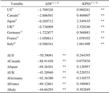
Before proceeding to the analysis of market integration one should look at the (non)stationary nature of the G7 se-ries. Unit root and stationarity tests in levels and in first differences for all the series are shown in Table 1.
As noted before, the ADF and KPSS tests are designed to capture weak stationarity with opposite null hypotheses. In the former case the null hypothesis of nonstationarity of the variables in levels is not rejected but it is rejected at 1% for the variables in first differences. In the latter case the null hypothesis of stationarity in levels is rejected at 1% but it is not rejected in first differences. The results are, therefore, consistent in both cases and lead to the conclusion that the price series under analysis are, in fact, integrated of first order. The number of lags selected in each test was set on the basis of the Schwarz Bayesian information Criterion (SBC) [32]. One can thus conclude that the stock price se-ries under analysis are nonstationary variables while stock
Table 1 Unit root and stationarity tests in levels and in first differences
Variable ADF a, c, d) KPSS b, c, d) USf) 1.709328 0.960241 ** Canadae) 2.806501 0.468607 ** Japanf) 0.269712 2.549435 ** UKg) 0.736909 2.320246 ** Germanye) 1.722877 0.568883 ** Francee) 1.050611 1.038102 ** Italyg) 0.500341 1.661498 ** US 70.39091 ** 0.244395 Canada 88.91458 ** 0.075838 Japan 69.26301 ** 0.126957 UK 45.20940 ** 0.220531 Germany 92.36380 ** 0.130575 France 89.32861 ** 0.186063 Italy 44.66293 ** 0.302849
a) MacKinnon (1996) critical values: 3.43 (1%) and 2.86 (5%) for constant and 3.96 (1%) and 3.41 (5%) for constant and linear trend; b) Kwiatkowski-Phillips-Schmidt-Shin (1992) critical values: 0.739 (1%) and 0.463 (5%) for constant and 0.216 (1%) and 0.146 (5%) for constant and linear trend; c) exogenous terms in levels: constant and linear trend; d) exogenous terms in 1st differences: constant (except for Japan in the KPSS test which is constant and linear trend); e) 1 lag in levels for ADF; f) 2 lags in levels for ADF; g) 4 lags in levels for ADF. ** Significant at 1%.
returns are stationary. Therefore, the analysis of stock mar-ket integration has to be conducted within the environment of cointegration.
The typical approach to cointegration in the context of multi-direction endogenous relationships is the specification of a VEC model, as described before. Testing procedures usually rely on the Johansen methodology which provides more powerful test statistics than the original Engle- Granger methodology in the presence of endogenous sys-tems. The Johansen tests are based on the rank of matrix , but also suffer from low power problems in the pres-ence of structural breaks because they assume that the coin-tegrating vector is time-invariant under the alternative hy-pothesis. This may lead to an over non-rejection of the null that the rank of is zero, thus leading the researcher to incorrectly conclude that there is no long-run relationship in the data. Structural breaks are likely to occur especially when we analyze relatively long time series, as is our case (daily data over 36 years), with shifts or the occurrence of extreme events (one or several) somewhere within the peri-od. Thus, formal tests for structural breaks are required.
To examine the statistical presence of structural breaks, we first performed cumulative sum (CUSUM) and cumula-tive sum of squares (CUSUM-Q) tests. As usual, we tested for the stability of our time series by regressing each of them on a nonsignificant constant. The results indicate the presence of structural breaks for all the variables and some of these structural breaks seem to be related to the occur-rence of stock market crashes and financial crises, reinforc-ing the possibility of nonlinear behavior among the stock markets under study. These tests, however, are best suited under a stationary environment.
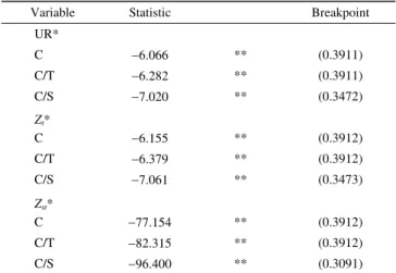
Under nonstationary structural breaks, an alternative to the Johansen method must be devised in order to test for cointegration without loss of statistical power. To this end, the Phillips (Zt and Zα) and unit root (UR) tests proposed by
Gregory and Hansen (GH) [33] are likely to constitute a good approach. The GH test statistics for cointegration are presented in Table 2.
The GH approach relies on a regression equation of the form:
1t
0
1 t
0 2 t
1 2 t t
t,x t x x u (8)
where the observed data is xt = (x1t, x2t), x2t is an m-vector of
variables, ut is a stationary error term, , s, s (s = 0, 1) are
parameters or vectors of parameters, t = 1,n, and t is a dummy variable that governs the structural change, so that
0 if , 1 if , t t n t n (9)where (0, 1) and [ ] denotes integer part. The unknown parameter symbolizes the relative timing of the break point [33].
Table 2 UR and Philips cointegration tests
Variable Statistic Breakpoint
UR* C 6.066 ** (0.3911) C/T 6.282 ** (0.3911) C/S 7.020 ** (0.3472) Zt* C 6.155 ** (0.3912) C/T 6.379 ** (0.3912) C/S 7.061 ** (0.3473) Z* C 77.154 ** (0.3912) C/T 82.315 ** (0.3912) C/S 96.400 ** (0.3091)
Gregory and Hansen (1996) critical values: 6.05 (1%) for C, 6.36 (1%) for C/T and 6.92 (1%) for C/S for the UR* and Zt* tests; 70.18
(1%) for C, 76.95 (1%) for C/T and 90.35 (1%) for C/S for the Z* test.
m = 6. ** Significant at 1%.
denoting just a change in the intercept . A level shift with trend occurs when 1 = 0 and 0 (C/T). Finally, when = 0 and 1 0 the model is called a regime shift (C/S), al-lowing the slope vector to shift as well.
The results reject the null hypothesis of no cointegration at the 1% level in all the tests and indicate that there is a breakpoint in the series at about 39% of the time period analyzed for the level shift and level shift with trend. A re-gime shift also occurs at about 31%–35% of the period. The level shift occurred in 1987 (black Monday) and the re-gime-shift occurred in 1984–1985. There is, therefore, no-table evidence that stock markets among the G7 are linked in the long-run, despite the incidence of shifts provoked by structural breaks resultant from crashes or other economic or financial distortions that change the market behavior in a “permanent” way. A first, but not surprising, conclusion is that stock market integration does happen for the G7, alt-hough at this point one cannot say whether this occurs in a weak or strong form.
On the light of the above cointegration tests and under the Granger Representation Theorem it is possible to speci-fy a VEC model with the guarantee that the residuals are stationary as required for inference purposes. Under these circumstances, the parameter estimates can be computed as usual and the t and F statistics can be used for testing pur-poses in the same way as in the case of a stationary OLS or Maximum Likelihood process. The VEC model allows for testing parameter restrictions on the -matrix that con-tains the long-run system information.
On the basis of the VEC estimates it is possible to test for the direction of causality that occurs in the system [10,34]. A popular test used in this context is the Granger causality [35]. Simple manipulation of the VEC leads to a
reparame-terized version of eq. (7) where the vector is multiplied by the estimated long-run residuals and the matrices Ai (i =
1,m) contain the coefficients of the lagged returns for each variable separately. For a two cointegrated variable system and p lags3), and noting that
1 ˆ 1
ˆt t
u β x one has
1 1, 2 2, ˆ1 ,
xt A x t jA x t j μut εt (10) where xt represents returns or log price changes at time t
and xi,tj (i = 1, 2; j = 1,p1) denotes lagged returns up
to p1 of the ith variable. A1 and A2 are [2(p1)] matrices. and t are (21) vectors and uˆt1 denotes the long-run residuals, where ut ~ I(0). A Granger causality test can be
carried out on the basis of the null hypothesis: i1 = =
i,p1 = i = 0, where the i coefficients correspond to the ith
row of A2. The test then compares the mean squared error under the null and under the alternative hypotheses, such that
ˆ1 1
ˆ1 1 2, 1
MSE xt |It MSE xt |It \Ix t , (11) where MSE is the mean squared error, It1 represents the set
of all past and present information existing at date t1,
Ix2,t1 represents the set of all past and present information existing on x2 at date t1, i.e. Ix2,t1 = {x21, x22,x2,t1}, x1t is the value of x1 at moment t (x1t It) and x is a non bi-ˆ1t
ased predictor of x1t. The Granger causality test is interpret-ed as follows: x2t Granger causes x1t if, ceteris paribus, the past values of x2t help to improve the current forecast of x1t. On the other hand, x2t instantaneously causes x1t in the sense of Granger if, ceteris paribus, the past and present values of
x2t help to improve the prediction of the current value of x1t, that is
ˆ1 1
ˆ1 2, 1
MSE xt |It\xt MSE xt|It\Ix t,xt . (12)
In practice, the Granger causality test performed in sta-tistical software postulates as the null hypothesis that “x2t does not Granger cause x1t”, so that causality implies the rejection of the null.
Table 3 presents the Granger causality tests for the varia-bles in levels, that is, stock prices. Here, x2t represents the variables in the first column and x1t represents the variables in the first row. One can say, therefore, that for the signifi-cant causal relationships the historical prices of the former market affect the current price of the latter, forming a dy-namical long-run relationship in the global economy. As we can see, about 74% of the coefficients are statistically sig-nificant, which means that there is substantial long-run causal effects among these markets, of which many of them are feedback relationships. However, we found no causal relationship in any direction for the pairs Germany-France
Table 3 Granger causality for log prices
Variable US Canada Japan
US 142.898 ** 716.963 ** Canada 36.0065 ** 361.477 ** Japan 14.3828 ** 4.86702 ** UK 8.91317 ** 3.99597 * 233.251 ** Germany 6.03121 ** 2.29723 284.715 ** France 9.72877 ** 1.51540 259.915 ** Italy 1.93860 1.01208 107.911 **
Variable UK Germany France
US 475.981 ** 390.273 ** 470.843 ** Canada 113.420 ** 73.5093 ** 117.433 ** Japan 27.3334 ** 21.9847 ** 24.1686 ** UK 7.33226 ** 6.02136 ** Germany 1.13299 2.17821 France 6.42979 ** 1.54816 Italy 0.61978 1.42051 7.52491 ** Variable Italy US 156.006 ** Canada 46.4521 ** Japan 7.23094 ** UK 3.54475 * Germany 0.32732 France 1.21910 Italy
H0: xit does not Granger cause xjt (i ≠ j); 2 lags; 9406 observations in
each series; ** significant at 1%; * significant at 5%.
and Germany-Italy which is a surprising result since we expected that European stock markets would co-move quite closely given the environment and political rules of the Eu-ropean Union, formerly EuEu-ropean Community.
Another important result is that, in the long-run, the US causes more than is caused by other markets. To see this, note that the F-statistics of the former (1st row) are substan-tially larger than the F-statistics of the latter (1st column). This is consistent with the idea that the US stock market, to a greater extent, ‘exports’ more than ‘imports’ boosts and crises, being therefore the engine of the global financial world. For example, a crisis with origin in the US can spread in a broader way to other markets (as it seems in the recent crisis) than a crisis with origin in Japan or even any European country. Canada shows an overall picture very similar to the US, that is, in general it causes more other markets than is caused by them, except in what refers to the US. Canada, however, appears to be caused only by the US, Japan and, to a lesser extent, the UK. Conversely, Japan is the most endogenous of the G7 markets. The European countries do not show an overall systematic pattern of cau-sality, though the UK appears to emerge like an attractor in the EU context (but not with France) and follows the North- American markets. This is also surprising insofar we would expect Germany to be the leading European stock market,
given its role as the ‘head’ of the European Union economy, albeit one should recognize the very important role of the London Stock Exchange in the global financial world.
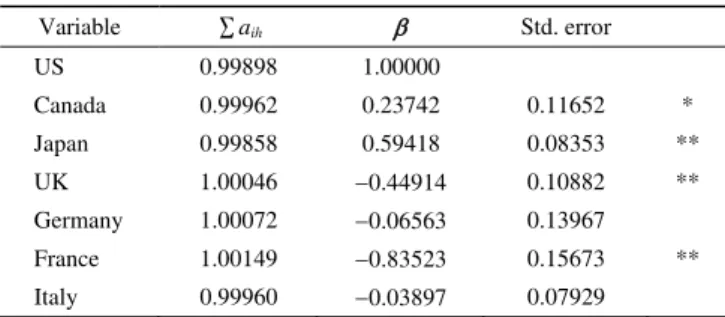
One may now proceed to the analysis of long-run market integration between market prices and returns in order to investigate whether the LOP holds for the system as a whole and/or for some of these markets bilaterally. Notice that if the LOP holds, strong market integration occurs in the sys-tem; otherwise there is weak market integration given that the variables are cointegrated, as shown before. The testing procedure considers the VAR estimates of the seven- country system in order to investigate whether price trans-mission is proportional or not. This test utilizes the sum of the VAR estimates for each equation in the system, where the null is H0:
iph1aih1, (aih Ak, k = 1,p). Theresults are presented in Table 4.
As can be seen, the sum of the VAR estimates is very close to one in all cases, suggesting (apparently) that strong long-run market integration occurs for the G7 system. These results may be checked using the long-run VEC estimates. The null hypothesis in this test postulates that β11 = 1 and
7 1
2 1.
k k Under the null hypothesis, the test statisticis 2(1) = 16.77231 (p = 0.000042) and therefore the null is rejected (the estimated β coefficients are reported in Table 4 along with the corresponding standard errors). This implies that market integration for the G7 only occurs in a weak form, that is, although some price transmission relationships may actually be linear (proportional transmission), there are cases where they are nonlinear (non-proportional transmis-sion) turning stock market interactions a complex system.
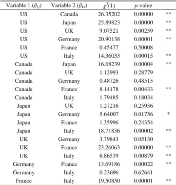
While being important to determine whether market in-tegration occurs for the system as a whole, it is also im-portant to know if shocks to the system propagate uniformly over the seven markets in analysis, in order to understand to what extent a shock affects the performance of the stock market. To this end, bivariate market integration tests must be conducted. The results of these tests are displayed in Table 5.
The test statistic follows a 2 distribution with one degree of freedom. The null hypothesis in this test indicates
Table 4 Long-run market integration tests for multivariate systems
Variable ∑aih Std. error
US 0.99898 1.00000 Canada 0.99962 0.23742 0.11652 * Japan 0.99858 0.59418 0.08353 ** UK 1.00046 0.44914 0.10882 ** Germany 1.00072 0.06563 0.13967 France 1.00149 0.83523 0.15673 ** Italy 0.99960 0.03897 0.07929
H0: ∑aih = 1; Exogenous terms in CE: constant; 2 lags in the
endoge-nous variables; 9405 observations after adjustments; ** significant at 1%; * significant at 5%.
Table 5 Long-run market integration tests for bivariate systems
Variable 1 (β1j) Variable 2 (β1k) 2(1) p-value
US Canada 26.35202 0.00000 ** US Japan 25.89823 0.00000 ** US UK 9.07521 0.00259 ** US Germany 20.90138 0.00001 ** US France 0.45477 0.50008 US Italy 14.36033 0.00015 ** Canada Japan 16.68239 0.00004 ** Canada UK 1.12993 0.28779 Canada Germany 0.48726 0.48515 Canada France 8.14178 0.00433 ** Canada Italy 1.79485 0.18034 Japan UK 1.27216 0.25936 Japan Germany 5.64007 0.01756 * Japan France 1.35996 0.24354 Japan Italy 18.71836 0.00002 ** UK Germany 3.79843 0.05130 UK France 23.26063 0.00000 ** UK Italy 6.86539 0.00879 ** Germany France 13.69186 0.00022 ** Germany Italy 0.23696 0.62641 France Italy 19.50850 0.00001 **
H0: β1j = 1, β1k = 1 (j ≠ k); Exogenous terms in CE: constant; 2 lags in
the endogenous variables; 9405 observations after adjustments; ** Signifi-cant at 1%; * signifiSignifi-cant at 5%.
proportionality or full price transmission over time. If the null hypothesis is not rejected then market j and market k are strongly integrated in the long-run. The null hypothesis is rejected in 62% of the bivariate relationships considered. Proportionality was only found for US-France, Canada-UK, Canada-Germany, Canada-Italy, Japan-UK, Japan-France, UK-Germany and Germany-Italy. For the remaining cases it was found that, in terms of pairwise relationships, although the underlying markets belong to the same market space, they are not related in a linear way. Such relationships are, therefore, much more complex and certainly some type of nonlinear relationship links the markets in the global world. For example, a shock in the US market is transmitted in a linear way only to France, while the transmission to other markets may be amplified or attenuated according to the impact factors given by the long-run coefficients.
4 Discussion and conclusions
This paper analyzes the stock market globalization on the basis of market integration among the G7 countries using a time-series approach based on logarithmic price relation-ships. Strong market integration occurs if shocks in one market are linearly (or proportionally) transmitted to anoth-er market (or othanoth-er markets). If transmission is nonlinear (or non-proportional) one can say that weak market integration holds. These definitions, of course, only apply if there is a non-spurious relationship between the variables under study.
Under nonstationarity, a cointegration system framework is used in order to obtain the relevant statistics. Structural breaks are also explicitly modeled. The results point to the following conclusions.
(1) There is an overall non-spurious relationship between the seven markets analyzed, given the rejection of the null of no cointegration. These markets thus belong to the same market space.
(2) The US market leads the G7 market space and the UK emerges as a regional attractor within the European context, which, in turn, is strongly affected by the North- American markets.
(3) Canada may benefit from its proximity to the US where, surely, intense economic relationships, some similar economic policies and firm’s relationships turn up the North American countries as a unified financial block. Canada, therefore, appears to show a dominant position in the mar-ket relatively to the non-American G7 countries.
(4) Japan does not emerge as a leading market within the G7 countries but this is probably due to the long-lasting economic crisis that Japan faced. Over the period analyzed Japan appears as the most endogenous market among the G7, which means that, while not affecting much the behav-ior of the other markets, the Japanese stock market is great-ly influenced by shocks occurring elsewhere within the G7.
(5) The continental European countries do not show an overall systematic pattern of causality, arising as ‘second-ary’ players in the global arena of stock markets within the G7.
(6) For the G7 system as a whole the null hypothesis of proportional price transmission is rejected. Furthermore, for more than 60% of the bivariate tests of proportionality the null is also rejected, which suggests that market integration occurs for the G7 countries in a weak form. This is im-portant insofar shocks occurring in the leading market, the US, are transmitted in quite different manners to the other markets, which turns quite difficult to devise common poli-cies in order to minimize the transmission of shock effects and stabilize markets overall.
As a final remark we argue that weak market integration is nothing but just an imperfect form of harmonization in the global world and that further deepening and develop-ment is needed in order to achieve strong market integra-tion.
This work was supported by FCT-Fundação para a Ciência e Tecnologia
(PTDC/GES/73418/2006, PTDC/GES/70529/2006, and FCOMP-01-0124-
FEDER-007350).
1 Arshanapalli B, Doukas J. Common stochastic trends in a system of eurocurrency rates. J Bank Finan, 1994, 18: 10471061
2 Chung P J, Liu D J. Common stochastic trends in Pacific Rim stock markets. Quart Rev Econom Finan, 1994, 34: 241259
3 Drożdż S, Grümmer F, Ruf F, et al. Towards identifying the world stock market cross-correlations: DAX versus Dow Jones. Physica A, 2001, 294: 226234
4 Hamao Y, Masulis R W, Ng V. Correlations in price changes and volatility across international stock markets. Rev Finan Stud, 1990, 3: 281307
5 Kasa K. Common stochastic trends in international stock markets. J Monet Econom, 1992, 29: 95124
6 Masih A M M, Masih R. Dynamic linkages and the propagation mechanism driving major international stock markets: An analysis of the pre- and post-crash eras. Quart Rev Econom Finan, 1997, 37: 859885 7 Masih A M M, Masih R. Propagative causal price transmission
among international stock markets: Evidence from the pre- and post- globalization period. Glob Finan J, 2002, 13: 6391
8 Tavares J. Economic integration and the comovement of stock returns. Econom Lett, 2009, 103: 6567
9 Zhou W, Sornette D. Evidence of a world-wide stock market log- pe-riodic anti-bubble since mid-2000. Physica A, 2003, 330: 543583 10 Alexander C. Practical Financial Econometrics—Market Risk
Analy-sis II. New York: John Wiley & Sons, 2008
11 Engle R F, Granger C. Cointegration and error-correction: Represen-tation, estimation and testing. Econometrica, 1987, 55: 251276 12 Eun C S, Shim S. International transmission of stock market
move-ments. J Finan Quant Anal, 1989, 24: 241256
13 Stigler G J. The Theory of Price. London: Macmillan, 1969
14 Sutton J. Sunk Costs and Market Structure. Cambridge: MIT Press, 1991
15 Bonfiglioli A, Favero C. Explaining co-movements between stock- markets: The case of US and Germany. J Int Money Finan, 2005, 24: 12991316
16 Corazza M, Malliaris A G, Scalco E. Nonlinear bivariate comove-ments of asset prices: Methodology, tests and applications. Comput Econom, 2010, 35: 123
17 Kim S J, Moshirian F, Wu E. Dynamic stock market integration driven by the European Monetary Union: An empirical analysis. J Bank Finan, 2005, 29: 24752502
18 Savva C. International stock markets interactions and conditional correlations. J Int Finan Mark Inst Money, 2009, 19: 645666 19 Cassel G. Abnormal deviations in international exchanges. Econom J,
1918, 28: 413415
20 Ross S A. The arbitrage theory of capital asset pricing. J Econom Theory, 1976, 13: 341360
21 Dickey D A, Fuller W A. Distribution of the estimators for auto-regressive time series with a unit root. J Am Stat Assoc, 1979, 74: 427431
22 Dickey D A, Fuller W A. Likelihood ratio statistics for autoregressive time series with a unit root. Econometrica, 1981, 49: 1057–1072 23 MacKinnon J G. Critical values for co-integration tests. In: Engle R F,
Granger C W J, eds. Long-Run Economic Relationships. Oxford: Oxford University Press, 1991. 267276
24 MacKinnon J G. Numerical distribution functions for unit root and cointegration tests. J Appl Econom, 1996, 11: 601618
25 Blough S R. The relationship between power and level for generic unit root tests in finite samples. J Appl Econom, 1992, 7: 295308 26 Kwiatkowski D, Phillips P C B, Schmidt P, et al. Testing the null
hypothesis of stationarity against the alternative of a unit root: How sure are we that economic time series have a unit root? J Econom, 1992, 54: 159178
27 Phillips P C B. Understanding spurious regressions in econometrics. J Econom, 1986, 33: 311340
28 Granger C W J, Newbold P. Spurious regressions in econometrics. J Econom, 1974, 2: 111120
29 Stock J H. Asymptotic properties of least squares estimation of coin-tegration vectors. Econometrica, 1987, 55: 10351056
30 Hendry D F, Juselius K. Explaining cointegration analysis: Part 1. Energy J, 2000, 21: 142
31 Beine M, Capelle-Blancard G, Raymond H. International nonlinear causality between stock markets. Europ J Finan, 2008, 14: 663686 32 Schwarz G. Estimating the dimension of a model. Ann Stat, 1978, 6:
461464
33 Gregory A, Hansen B. Residual-based tests for cointegration in mod-els with regime shifts. J Econom, 1996, 70: 99126
34 Hart P E, Mills G, Whitaker J K. Econometric Analysis for National Economic Planning (Colston Papers No. 16). London: Butterworths, 1964
35 Granger C W J. Investigating causal relations by econometric models and cross-spectral methods. Econometrica, 1969, 37: 424438
Open Access This article is distributed under the terms of the Creative Commons Attribution License which permits any use, distribution, and reproduction