For Peer Review Only
Uncertainty measures application in the training and evaluation of supervised classifiers
Journal: International Journal of Remote Sensing Manuscript ID: TRES-PAP-2010-0083.R2
Manuscript Type: IJRS Research Paper Date Submitted by the
Author: 11-Jul-2010
Complete List of Authors: Gonçalves, Luisa M S; Polytechnic Institute of Leiria, Department of Civil Engineering
Fonte, Cidália C; University of Coimbra, Department of Mathematics Júlio, Eduardo N B S; University of Coimbra, ISISE, Civil
Engineering Department
Caetano, Mário; Portuguese Geographic Institute (IGP), Remote Sensing Unit (RSU), Lisboa, Portugal
Keywords: IKONOS, FUZZY CLASSIFICATION, THEMATIC MAPPING Keywords (user defined): Uncertainty measures, Training Areas, Accuracy assessment
For Peer Review Only
Catchline (head of first page only) Journal name in full, Vol. X, No. X, Month 2010, xxx–xxx
Running heads
(verso)
Gonçalves, Fonte, Júlio and Caetano
(recto)
Uncertainty application in classifiers training and evaluation
Article Type (Research Paper)
Uncertainty measures application in the training and evaluation of
supervised classifiers
LUISA M.S. GONÇALVES*†¶, CIDÁLIA C. FONTE §¶, EDUARDO N.B.S. JÚLIO&, MARIO
CAETANO‡
†Civil Engineering Department, Polytechnic Institute of Leiria, Portugal
¶Institute for Systems and Computers Engineering at Coimbra, Portugal§Department of Mathematics, University of Coimbra, Portugal
&ISISE, Civil Engineering Department, University of Coimbra, Portugal
‡Portuguese Geographic Institute (IGP), Remote Sensing Unit (RSU), Lisboa, Portugal
‡ Institute for Statistics and Information Management (ISEGI), Universidade Nova de Lisboa, Lisboa,
Portugal
*†Email: [email protected]
Abstract
The production of thematic maps from remotely sensed images requires the application of classification methods. A great variety of classifiers is available, producing frequently considerably different results. Therefore, the automatic extraction of thematic information requires the choice of the most appropriate classifier for each application. One of the main objectives of the research described in this paper is to evaluate the performance of supervised classifiers using the information provided by the application of uncertainty measures to the testing sets, instead of statistical accuracy indices. The second main objective is to show that the information provided by the uncertainty measures for the training set may be used to assess and redefine the sample sites included in this set, in order to improve the classification results. To achieve the proposed objectives, two supervised classifiers, one probabilistic and another fuzzy, were applied to a Very High Spatial Resolution (VHSR) image. The results show that similar conclusions on the classifiers performance are obtained with the uncertainty measures and the traditional accuracy indices obtained from error matrixes. It is also shown that the redefinition of the training set based on the information provided by the uncertainty measures may generate more accurate outputs.
Keywords:
Uncertainty measures; Training areas; Accuracy assessment
3 4 5 6 7 8 9 10 11 12 13 14 15 16 17 18 19 20 21 22 23 24 25 26 27 28 29 30 31 32 33 34 35 36 37 38 39 40 41 42 43 44 45 46 47 48 49 50 51 52 53 54 55 56 57 58
For Peer Review Only
AMS Subject Classification:
1 Introduction
The classification of remote sensing images may be performed with several methods, which have different characteristics and are based on different assumptions. The supervised classifiers perform the classification considering the spectral responses of the training samples chosen in regions considered representative of each identified class in the image. The classification procedure includes three phases. The first corresponds to the identification of training areas in the image for each class, which are used as descriptors of the spectral characteristics of the classes. This information is then used to assign each spatial unit of the image (usually a pixel or an object) to a class or to several classes if soft classifiers are used. The last phase is the validation of the obtained results. Since different classifiers usually give different classification results, to choose the appropriate classifier for each data set and nomenclature it is necessary to determine first which classifiers are the most adequate.
Traditionally the evaluation of the classifiers behaviour is performed considering an additional sample of points within the regions representative of the classes, evaluating the accuracy of the classification for those points, constructing an error matrix and computing accuracy indices for the classes, such as the User Accuracy (UA) and the Producer Accuracy (PA), and global indices, such as the Overall Accuracy and the KHAT value (an estimator of the kappa coefficient) (Congalton and Green 1999). However, this approach is very demanding in terms of human and financial resources, and often is made only at the end of the methodological process. In addition it has also some drawbacks: (1) it requires the identification of the ground truth for an additional sample of points, which is always a time consuming operation (Gopal and Woodcock 1994; Gonçalves et al. 2010); (2) it is influenced by the sampling methods and sample size (Stehman and Czaplewski 2003); (3) it is influenced by a certain degree of subjectivity of the reference data (Plantier and Caetano 2007); (4) it is only appropriate for traditional methods of classification, where it is assumed that pixels at the reference locations can be assigned to a single class (Lewis and Brown 2001); and (5) it cannot provide spatial information of where thematic errors occur (Brown et al. 2009).
In remote sensing, classifiers that provide additional information about the difficulty in identifying the best class for each pixel have been developed, such as the posterior probabilities of the maximum likelihood classifier (Foody et al. 1992; Bastin 1997; Ibrahim et al. 2005; Gonçalves et al. 2009a), the grades of membership of fuzzy classifiers (Stehman 2001; Foody 1996; Bastin 1997; Zhang and Kirby 1999), and the strength of class membership when classifiers based on artificial neural networks are used (Foody 1996; Zhang and Foody 2001; Brown et al. 2009). These classification methods assign, to each pixel of the image and to each class, a probability, possibility or degree of membership (depending on the considered assumptions and mathematical theories used). This may be interpreted as partial membership of the pixel to the classes (as in the case of mixed pixels or objects), a degree of similarity between what exists on the ground and the pure classes, or the uncertainty associated with the classification. In any of these cases, this additional information also reflects the classifier’s difficulties in identifying which class should be assigned to the pixels, and therefore it may be processed as uncertainty information. Different approaches to assess the accuracy of these classifications have been proposed (Foody 1996; Arora and Foody 1997; Binaghi et al. 1999; Woodcock and Gopal 2000; Lewis and Brown 2001; Oki et al. 2004; Pontius and Connors 2006). However, several of these approaches are based on generalized cross tabulation matrices from which a range of accuracy measures, with similarities to those widely used with hard classifications may be derived (Doan and Foody 2007). Since for these classifiers, either a probability or possibility distribution is associated to each pixel, uncertainty measures may be applied to them, expressing the difficulty in assigning one class to each pixel, enabling an evaluation of the classification uncertainty and providing the user with additional valuable data to take decisions.
Uncertainty measures, among which the Shannon entropy is the most frequently used, have already been used by several authors to give an indication of the soft classification reliability (Maselli et al. 1994; Zhu 1997; Gonçalves 2009). In this paper one of the main objectives, is to investigate if the adequability of probabilistic and fuzzy classifiers can be assessed with the uncertainty information provided by the classifiers and the uncertainty indices, instead of using confusion matrices and accuracy indices at the initial stages of the classification. This approach presents the advantage of allowing the evaluation of the classifiers behaviour during the classification process without needing ground truth and, therefore, it can be used when ground truth samples are not available or too expensive to be obtained. In addition, 3 4 5 6 7 8 9 10 11 12 13 14 15 16 17 18 19 20 21 22 23 24 25 26 27 28 29 30 31 32 33 34 35 36 37 38 39 40 41 42 43 44 45 46 47 48 49 50 51 52 53 54 55 56 57 58 59
For Peer Review Only
with this approach all pixels inside the regions identified as corresponding to perfect examples of each class can be used to evaluate the classifiers, instead of using only a training sample inside these regions. Therefore, the results are only influenced by the regions chosen as corresponding to each of the classes and the human subjective influence is minimized.
The behaviour of a supervised classifier is influenced by a set of factors, such as the training sample, the nomenclature and the images characteristics (Foody et al. 2006). Several studies have already been conducted regarding the definition of sampling protocols and sample size that should be used in the training phase (Stehman 2001; Cochran 1977; Stehman and Czaplewski 2003; Foody et al. 2006). However, improvements are still needed in this area, namely in the selection of the training sample, since it is always a complex process and frequently requires successive improvements. The second main objective of this research is to investigate if, after an initial classification, the information provided by the uncertainty measures for the training set may be used to redefine this set, removing less reliable samples and improving the final classification accuracy. This approach enables the use of an automatic method to assist the selection of training samples. To achieve these objectives a methodology was developed that includes the following steps: (1) definition of the sampling protocol; (2) selection of the training and testing sample for each class; (3) classification allocation using soft classifiers; (4) computation of uncertainty measures for the training and testing set; (5) evaluation of the classifiers using uncertainty indices obtained for the testing set; (6) redefinition of the training set using the information provided by the uncertainty measures; (7) repetition of step 3; (8) evaluation of the accuracy of the classification obtained in the previous step.
2 Data
The study was conducted in a rural area with a smooth topographic relief, featuring diverse landscapes representing Mediterranean environments. An image obtained by the IKONOS sensor was used (Figure 1), with a spatial resolution of 4m in the multi-spectral mode (XS). The product acquired was the Geo Ortho Kit and the study was performed using the four multi-spectral bands. The geometric correction of the multi-spectral image consisted of its orthorectification. The average quadratic error obtained for the geometric correction was of 1.39m, less than half the pixel size, which guarantees an accurate geo-referencing. The acquisition details of the image are presented in Table 1.
‘ – Place Figure 1 here – ’ ‘ – Place Table 1 here – ’
3 Methodology
In this study, before the classification itself, various preliminary processing steps were carried out. First, an analysis of the image by a human interpreter was made to define the most representative classes. The classes used in this study are the following: Eucalyptus Trees (ET); Cork Trees (CKT), Coniferous Trees (CFT); Shadows (S); Shallow Water (SW), Deep Water (DW), Herbaceous Vegetation (HV), Sparse Herbaceous Vegetation (SHV) and Non-Vegetated Area (NVA). The following step was the establishment of the sample protocol to select the training and testing sample elements. The training and testing dataset consisted in a semi-random selection of sites. A human interpreter delimited twenty five polygons for each class and a stratified random selection of 300 samples per class was performed. One half of this points was used to train the classifier and the other half, presenting a spectral variability in class response very similar to the training set, was used to evaluate the classifier’s behaviour. The sample unit was the pixel. The total sample size used for training included 1350 pixels. An equal number of pixels was used to test the classifier accuracy. Only pixels representative of pure classes were considered (Plantier and Caetano 2007). The two classifications were then performed, with a supervised classifier based on the maximum likelihood classifier and a supervised fuzzy classifier based on the underlying logic of Minimum-Distance-to-Means classifier. The uncertainty measures were computed for the polygons identified as corresponding to each of the classes. To determine if the information given by the uncertainty measures was consistent with the accuracy indices, an error matrix was made with the testing set and the Overall Accuracy was computed, as well as the KHAT value. The User Accuracy (UA) and the Producer Accuracy 3 4 5 6 7 8 9 10 11 12 13 14 15 16 17 18 19 20 21 22 23 24 25 26 27 28 29 30 31 32 33 34 35 36 37 38 39 40 41 42 43 44 45 46 47 48 49 50 51 52 53 54 55 56 57 58
For Peer Review Only
(PA) indices were also computed for all classes. The reference data were obtained from aerial images with finer spatial resolution. The conclusions obtained from both approaches were then compared.
Since the operation of supervised classifiers depends on the training stage, the definition of the training set may be optimized in order to improve the classification accuracy, so that the used samples characterize appropriately the spectral response of the class. To this aim, after the initial soft classification, the main problems of the classification that could have an origin on the selection of the training set were identified. After this evaluation, a reselection of the training sites was made for the classes that present higher uncertainty with the preliminary first classification, eliminating the samples that present higher levels of uncertainty. The main goal of this approach is to avoid the use of the training sites which presented a higher deviation from the predominant characteristics of the class signature. To evaluate if the redefinition of the training set based on uncertainty information improved the classifier behaviour, which was one of the goals of the study, a comparison between the classifiers accuracy obtained before and after the redefinition of the training set was made.
3.1 Classifiers
The first classification method used is based on the maximum likelihood classifier (Bayes classifier), which depends on the estimation of the multivariate Gaussian probability density function of each class using the classes statistics (mean, variance and covariance) estimated from the sample pixels of the training set. The probability density function is given by (Foody et al., 1992), =
(
− (
−)
−(
−)
)
π T 1 1 / 2 / 2 1 ( | ) exp 1 / 2 (2 )k i i i i p x i V V ΧΧΧΧ µµµµ ΧΧΧΧ µµµµ (1)where p x i( | ) is a probability density function of a pixel x as a member of class i, k is the number of bands, X is the
vector denoting the spectral response of pixel x, Vi is the variance-covariance matrix for class i and µµµµiis the mean
vector over all training pixels of class i.
The traditional use of this classification method assigns each pixel to the class corresponding to the highest probability density function value. However, the posterior probabilities can be computed from the probability density functions. The posterior probabilities of a pixel x belonging to class i, denoted by ( )p x , is given by Equation 2, i
= =
∑
1 ( ) ( | ) ( ) ( ) ( | ) i n i P i p x i p x P i p x i (2)where P i( ) is the prior probability of class i(the probability of the hypothesis being true regardless of the evidence) and n is the number of classes. These posterior probabilities sum up to one for each pixel (Foody et al. 1992), and may be
interpreted as representing the proportional cover of the classes in each pixel or as indicators of the uncertainty associated with the pixel allocation to the classes (Shi et al. 1999; Ibrahim et al. 2005). In this paper, this second interpretation is used, and the posterior probabilities are used to compute uncertainty measures.
The second classification method used is a pixel-based supervised fuzzy classifier based on the underlying logic of the Minimum-Distance-to-Means classifier, available in the commercial software IDRISI. With this method, an image is classified based on the information contained in a series of signature files and a standard deviation unit (Z-score distance) chosen by the user. The fuzzy set membership is calculated based on a standardized Euclidean distance from each pixel reflectance, on each band, to the mean reflectance for each class signature, using a sigmoid membership function (Burrough and McDonnell 1998; Kuncheva 2000). The underlying logic is that the mean of a given signature represents the ideal point for the class, where fuzzy set membership is one. When distance increases, fuzzy set membership decreases, until it reaches the user-defined Z-score distance where fuzzy set membership decreases to zero. To determine the value to use for the standard deviation unit, the information of the training data set was used to study the spectral separability of the classes and to determine the average separability measure of the classes.
With this classification methodology, the sum of the degrees of membership of each pixel to each class may sum up to any value between zero and the number of classes. Since fuzzy sets induce possibility distributions (Klir 2004), a possibility distribution associated to each pixel is obtained.
3 4 5 6 7 8 9 10 11 12 13 14 15 16 17 18 19 20 21 22 23 24 25 26 27 28 29 30 31 32 33 34 35 36 37 38 39 40 41 42 43 44 45 46 47 48 49 50 51 52 53 54 55 56 57 58 59
For Peer Review Only
Unlike traditional hard classifiers, the output obtained with these classifiers is not a single classified map, but rather a set of images (one per class) that expresses the probability, for the first classifier, and the possibility, for the second one, that each pixel belongs to the class in question.
3.2 Classifiers evaluation
The evaluation of the classifiers behaviour was made using uncertainty measures. To evaluate the uncertainty of the probabilistic classifier, the Relative Maximum Deviation (R) and the Relative Probability Entropy (En) uncertainty
measures were used. To evaluate the uncertainty of the possibilistic classifier, the non-specificity measures Un and R
were used. An overview of the uncertainty measures used follows.
3.2.1 Entropy
The Shannon entropy measure (E), derived from Shannon’s information theory, is computed using Equation 3 (Ricotta 2005), 2 1 ( ) n i( )log i( ) i E x p x p x = = −
∑
(3)where ( )p x are the posterior probabilities of a pixel x for the i i classes and
n
is de number of classes. This measure Eassumes values in the interval [0,log n2 ]. Since several measures are considered in this study, a comparison between the results given by them is necessary, which is not possible if the measures have different ranges. Therefore, to overcome this problem, the measure En was used, which is similar to the one proposed by Maselli et al. (1994), and is given by
Equation 4, 1 2 2 ( )log ( ) ( ) log n i i i n p x p x E x n = − =
∑
(4)En varies between zero and one, meaning, for the value zero that there is no ambiguity in the assignment of the pixel to a
class, and therefore no uncertainty, and the value one, that the ambiguity is maximum.
3.2.2 U-uncertainty measures
Non-specificity measures have been developed within the context of possibility theory and fuzzy sets theory, namely, the U-uncertainty measure, proposed by Higashi and Klir (1982). This measure can be applied to fuzzy sets and to ordered possibility distributions and it is appropriate to evaluate the uncertainty resulting from possibilistic classifications, since it quantifies the ambiguity in specifying an exact solution (Pal and Bezdek 2000).
The U-uncertainty measure, proposed by Higashi and Klir (1982), applied to an ordered possibility distribution
(
) (
)
Π z z1, ,...,2 zn = π π1, ,...,2 πn , such that π1≥π2≥K≥πn, is given by Equation 5 (Mackay et al. 2003),
( )
Π[
π]
[
π π +]
= = − 1 2 +∑
− 1 2 2 1 log n i i log i U n i (5)where πi+1 is assumed to be zero.
Properties of this measure can be found in Pal and Bezdek (2000) or Klir (2000). From these properties, it can be stressed that for a universal set Z and a possibility distribution Π ,0≤U
( )
Π ≤log2n, where the minimum is obtainedfor Π
(
z z1, ,...,2 zn)
=(
1, 0,..., 0)
and the maximum value for Π(
z z1, ,...,2 zn)
=(
α α, ,...,α)
, ∀ ∈α[ ]
0,1 .A normalized version of this measure proposed by Gonçalves et al. (2010) is used in this paper, varying within the interval [0,1] and given by Equation 6,
( )
( )
( )
( )
1 2 1 2 2 2 1 log log log n i i i n x n x x i U x n π π π Π = + − + − = ∑
(6) whereπ1( )
x , π2( )
x ,…, πn( )
x are the ordered possibilities that pixel x be assigned to the n classes.3 4 5 6 7 8 9 10 11 12 13 14 15 16 17 18 19 20 21 22 23 24 25 26 27 28 29 30 31 32 33 34 35 36 37 38 39 40 41 42 43 44 45 46 47 48 49 50 51 52 53 54 55 56 57 58
For Peer Review Only
3.2.3 Relative Maximum Deviation Measure
The Relative Maximum Deviation Measure (R) is an uncertainty measure provided in IDRISI commercial software, which can be applied to both probability and possibility distributions, and is defined as shown in Table 2.
‘ – Place Table2 here – ’
This uncertainty measure assumes values in the interval [0,1]. The numerator of the second term expresses the difference between the maximum probability or possibility assigned to a class and the probability or possibility that would be associated with the classes if a total dispersion for all classes occurred. The denominator expresses the extreme case of the numerator, where the maximum probability or possibility is one (and thus a total commitment to a single class occurs). The ratio of these two quantities expresses the degree of commitment to a specific class in relation to the largest possible commitment (Eastman 2006). The classification uncertainty is thus the complement of this ratio and evaluates the degree of compatibility with the most probable or possible class and until which point the classification is dispersed over more than one class.
4. Results and discussion
4.1 Classifiers evaluation with accuracy indices
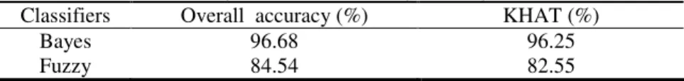
Table 3 shows the KHAT and the Overall Accuracy obtained from the testing set for the fuzzy and Bayes classifications. Table 4 and Table 5 present the confusion matrixes built.
‘ – Place Table 3 here – ’ ‘ – Place Table 4 here – ’ ‘ – Place Table 5 here – ’
According to both Overall Accuracy indices, the two classifiers present good results. However, both indices present better results for the Bayes classifier. Figures 2 and 3 show the results obtained for the UA and PA indices for both classifiers, ordered with increasing values for the fuzzy classifier.
‘ – Place Figure 2 here – ’ ‘ – Place Figure 3 here – ’
These Figures show that, for the Bayes classifier, UA and PA have values larger than 90%, for all classes. The classes with lower accuracy are CKT and SHV. Since the accuracy indices presented very high values for all classes, it may be concluded that the Bayes classifier has a good performance in their identification.
The results obtained for the fuzzy classifier are worse. Only the classes HV, S and DW have UA and PA larger than 90%. Moreover, all classes except the S class present lower values of UA and PA than the Bayes classifier. The class with the smallest value of PA is SW (62%), which means that is the class with more omission errors. The pixels that are erroneously not included in this class are included in the NVA class, which is the class with smallest UA (57%) and therefore the class with more commission error, receiving pixels from all classes. This shows that this classifier presents great difficulty in classifying NVA and SW classes.
4.2 Classifiers evaluation with uncertainty measures
Figure 4 shows the mean uncertainty per class obtained with R and En uncertainty measures for the probabilistic
classification, ordered with increasing values of R. Figure 5 shows the spatial distribution of the uncertainty values grouped into five levels, corresponding to 0% and to quartiles.
3 4 5 6 7 8 9 10 11 12 13 14 15 16 17 18 19 20 21 22 23 24 25 26 27 28 29 30 31 32 33 34 35 36 37 38 39 40 41 42 43 44 45 46 47 48 49 50 51 52 53 54 55 56 57 58 59
For Peer Review Only
‘ – Place Figure 4 here – ’‘ – Place Figure 5 here – ’
Figure 4 shows that the values of the mean uncertainty per class are very low, always less than 0.12. The classes that show higher levels of uncertainty are CKT and SHV. Figure 5 shows that the majority of samples have uncertainty values in the interval 1-25%. The information provided by the uncertainty measures is therefore in accordance with the one provided by the accuracy indices. The results also highlight that the information obtained with both measures are almost identical and the correlation between the two measures is very high (always larger than 0.95) (Figure 6).
‘ – Place Figure 6 here – ’
Figure 7 shows the mean uncertainty per class obtained with the Un and R uncertainty measures applied to the fuzzy
classification, ordered with increasing values of R. Figure 8 shows the spatial distribution of uncertainty values grouped into five levels, corresponding to 0% and to quartiles.
‘ – Place Figure 7 here – ’ ‘ – Place Figure 8 here – ’
The values of the mean uncertainty obtained with the uncertainty measures R and Un for the fuzzy classification, shown
in Figure 7, vary between 0.30 and 0.55. The values obtained with both uncertainty measures are in general very close and the correlation between the two measures is very high (always larger than 0.95) (Figure 9). The classes NVA and SW were the ones with higher uncertainty levels. Since with this classifier the uncertainty values are relatively high, an additional analysis of the possibility distributions associated with the pixels of the test sample was made to understand why the uncertainty values were so large. This analysis showed that, for all classes, there are a large percentage of pixels with relatively low values for the largest degree of possibility. For example, 25% of the sample pixels assigned to the DW class have the largest degree of possibility smaller than 0.5, which explains the high values of uncertainty. Moreover, no pixel of the testing sample has the largest possibility equal to 1 (maximum possibility).
For all classes, except NVA, the second degree of possibility was assigned to the NVA class with degrees of possibility frequently very close to the maximum. This means that there is great confusion between NVA and the other classes, which is one of the main problems of the application of this classifier to this case study. This conclusion was also obtained from the accuracy indices, since the NVA class presented a very large difference between the UA (57.3%) and the PA (97.4%). This means that this class presents a large number of commission errors and, therefore, samples that were assigned to the NVA class should have been assigned to other classes, such as SW and SHV, as it can be concluded from the error matrix (see Table 4) explaining why they have larger omission errors.
‘ – Place Figure 9 here – ’
4.3 Fuzzy Classifier evaluation with accuracy indices after redefining the training areas
According to both the accuracy and the uncertainty indices, the training set used for the Bayes classifier has a good performance, and therefore no changes to this set were made. However, according to both the accuracy indices and the uncertainty indices, some problems were found when using the sample set with the fuzzy classifier (some classes have relatively low accuracy, such as NVA, and also high uncertainty). For this reason, the training set used for the class NVA, which was the class identified as the most problematic, was redefined. This was done by excluding the sample sites with uncertainty higher than 0.5, which resulted in the redefinition of 52 sample sites. The fuzzy classification was then redone and the results evaluated computing the accuracy indices for the testing set. Table 6 presents the confusion matrix built. The resulting Overall Accuracy is 92%, which revealed an increase of 8%. Figure 10 and Figure 11 allow the comparison between the results for the UA and PA before and after the redefinition of the NVA training areas. 3 4 5 6 7 8 9 10 11 12 13 14 15 16 17 18 19 20 21 22 23 24 25 26 27 28 29 30 31 32 33 34 35 36 37 38 39 40 41 42 43 44 45 46 47 48 49 50 51 52 53 54 55 56 57 58
For Peer Review Only
‘ – Place Table 6 here – ’‘ – Place Figure 10 here – ’ ‘ – Place Figure 11 here – ’
Almost all classes presented a decrease of the commission errors, and especially the NVA class. The UA of the NVA class increased from 57% to 95.7%, only the SW and HV presented a slight increase of commission errors. The SW class, which was the class with more omission errors after the redefinition of the training samples, presented an increase of the PA accuracy from 62% to 100%. The NVA was the only class that presented a slight decrease of the PA.
In this case, the use of the classification uncertainty proved to be valuable in the process of selecting the training set. In fact, this strategy allowed the identification of the training sites which presented a higher deviation of the mean reflectance of the NVA class signature, avoiding their use in the classifier training phase. The redefinition of the NVA training set also influenced the accuracy of the other classes and allowed the improvement of the classifier behaviour. The obtained results showed that this approach is promising and worthy of further studies. Figure 12 shows the final results obtained with the classifiers using the proposed methodology.
‘ – Place Figure 12 here – ’
A relevant objective of this study was to show that uncertainty measures can be used: (1) to give a preliminary evaluation of the classifiers difficulties, (2) as an intermediate step between the classification and the generation of error matrixes, (3) to contribute to an iterative improvement of the classification process, identifying classes with higher levels of uncertainty and enabling the implementation of measures to improve the classification behaviour, which will result in accuracy improvement.
5. Conclusions
The results obtained with both classifiers show that the information about the uncertainty of the classification of regions considered as representative of the several classes can be used, together with the degrees of probability or possibility assigned to each pixel, to detect the main problems of the classifiers. For both classifiers, the same evaluation methodology was used to reach conclusions concerning the performance of the classifiers with the accuracy indices and the uncertainty information. Since it is very simple to apply the uncertainty measures to the probability or possibility distributions, this approach allows a much faster and cheaper evaluation of the classifiers’ performance than with accuracy indices. Also, unlike the accuracy results, they are not influenced by the subjectivity of the reference data. Besides that, they can be applied to all pixels of the regions chosen as representative of the several classes, since no reference information is necessary, which means that the influence of the sampling process is also excluded. It was also concluded that the information of the uncertainty can be very useful to the choice of the training areas. The behaviour of the fuzzy classifier improved 8% after the redefinition of the training areas of the classes NVA based on the uncertainty information associated with the training sites.
For all the reasons mentioned, it can be stated that the proposed approach is quite promising, since it provides valuable information to the user and it can reduce time and costs, deserving therefore further attention.
References
ARORA, M. K. and FOODY, G. M., 1997, Log-linear modelling for the evaluation of the variables affecting
the accuracy of probabilistic, fuzzy and neural network classifications. International Journal of
Remote Sensing
, 18, 785–798.
BASTIN, L., 1997, Comparison of fuzzy c-means classification, linear mixture modeling and MLC
probabilities as tools for unmixing coarse pixels. International Journal of Remote Sensing, 18,
3629-3648.
BINAGHI, E., BRIVIO, P.A., GHEZZI, P. and RAMPINI, A., 1999, A fuzzy set-based accuracy assessment
of soft classification. Pattern Recognition Letters, 20, 935-948.
3 4 5 6 7 8 9 10 11 12 13 14 15 16 17 18 19 20 21 22 23 24 25 26 27 28 29 30 31 32 33 34 35 36 37 38 39 40 41 42 43 44 45 46 47 48 49 50 51 52 53 54 55 56 57 58 59
For Peer Review Only
BURROUGH, P.A and MCDONNELL, R. A., 1998, Principles of Geographical Information Systems
(Oxford University Press: New York).
BROWN, K.M., FOODY, G.M. and ATKINSON, P.M., 2009, Estimating per-pixel thematic uncertainty in
remote sensing classifications. International Journal of Remote Sensing, 30, 209-229.
COCHRAN, W. G., 1977. Sampling Techniques, 3rd edition, (New York: Wiley).
CONGALTON,
R.G. and GREEN,
K., 1999, Assessing the accuracy of remotely sensed data: principles and
practices. (Boca Raton, FL: CRC/ Lewis Press).
DOAN, H. T. X. and FOODY, G. M., 2007, Increasing soft classification accuracy through the use of an
ensemble of classifiers. International Journal of Remote Sensing, 28, 4609-4623.
EASTMAN, J.R., 2006, IDRISI Andes Guide to GIS and Image Processing. Clark Labs., Clark University.
FOODY, G.M., CAMPBELL, N.A., TRODD, N.M. and WOOD, T.F., 1992, Derivation and applications of
probabilistic measures of class membership from maximum likelihood classification.
Photogrammetric Engineering and Remote Sensing
, 58, 1335-1341.
FOODY, G. M., 1996, Approaches for the production and evaluation of fuzzy land cover classifications from
remotely-sensed data. International Journal of Remote Sensing, 17, 1317-1340.
FOODY, G.M., MATHUR, A., SANCHEZ-HERNANDEZ, C. and BOYD, D.S., 2006, Training set size
requirements for the classification of a specific class. Remote Sensing of Environment, 104, 1-14.
GONÇALVES, L.M.S., 2009, Integração da incerteza na classificação e avaliação da exactidão temática de
imagens multiespectrais - Aplicação à avaliação de estudo de conservação do património edificado da
baixa de Coimbra. PhD. dissertation, Universidade de Coimbra, Coimbra.
GONÇALVES, L.M.S., FONTE, C.C., JÚLIO, E.N.B.S. and CAETANO, M., 2009 a, A method to
incorporate uncertainty in the classification of remote sensing images. International Journal of Remote
Sensing
, 30, 5489–5503.
GONÇALVES, L.M.S., C.C. FONTE, E.N.B.S. JÚLIO and M. CAETANO, 2010, Evaluation of soft
possibilistic classifications with non-specificity uncertainty measures. International Journal of Remote
Sensing, 31
, 5199-5219.
GOPAL, S. and C.E. WOODCOCK, 1994, Theory and methods for accuracy assessment of thematic maps
using fuzzy sets. Photogrammetric Engineering and Remote Sensing, 60,181-188.
HIGASHI, M., KLIR, G., 1982, Measures of uncertainaty and information based on possibility distribuitions.
International Journal of General Systems
, 9, 43- 58.
IBRAHIM, M. A., ARORA, M. K. and GHOSH, S. K., 2005, Estimating and accommodating uncertainty
through the soft classification of remote sensing data. International Journal of Remote Sensing, 26,
2995-3007.
KUNCHEVA, I.L, 2000, Fuzzy Classifier Design, (Heidelberg, New York: Physica-Verlag)
KLIR, G., 2000, Measures of uncertainty and information. In: Fundamentals of Fuzzy Sets, Dubois, D., Prade,
H. (eds.), pp. 439-457. (The Handbook of Fuzzy Sets Series, Kluwer Acad. Publ).
KLIR, G., 2004, Generalized information theory: aims, results and open problems. Reliability Engineering
and Systems Safety
, 85, 21-38.
3 4 5 6 7 8 9 10 11 12 13 14 15 16 17 18 19 20 21 22 23 24 25 26 27 28 29 30 31 32 33 34 35 36 37 38 39 40 41 42 43 44 45 46 47 48 49 50 51 52 53 54 55 56 57 58
For Peer Review Only
LEWIS, H.G. and BROWN, M., 2001. A generalized confusion matrix for assessing area estimates from
remotely sensed data. International Journal of Remote Sensing, 22, 3223-3235.
MACKAY, D., SAMANTA, S., AHL, D., EWERS, B., GOWER, S. and BURROWS, S., 2003, Automated
Parameterization of Land Surface Process Models Using Fuzzy Logic. Transaction in GIS, 7, 139-153.
MASELLI, F., CONESE, C., and PETKOV, L., 1994, Use of probability entropy for the estimation and
graphical representation of the accuracy of maximum likelihood classifications. ISPRS Journal of
Photogrammetry and Remote Sensing
, 49, 13-20.
OKI, K., UENISHI, T.M., OMASA, K. and TAMURA, M., 2004, Accuracy of land cover area estimated
from coarse spatial resolution images using an unmixing method. International Journal of Remote
Sensing
, 25, 1673–1683.
PAL, N., BEZDEK, J., 2000, Quantifying different facets of fuzzy uncertainty. In Fundamentals of Fuzzy
Sets,
Dubois, D., Prade, H. (eds.), pp. 459-480. (The Handbook of Fuzzy Sets Series, Kluwer Acad.
Publ).
PLANTIER, T. and CAETANO, M., 2007, Mapas do Coberto Florestal: Abordagem Combinada
Pixel/Objecto. In: J. Casaca and J. Matos (eds.) V Conferência Nacional de Cartografia e Geodesia,
Lisboa, Lidel, pp. 157-166.
PONTIUS, R.G. and CONNORS, J., 2006, Expanding the conceptual, mathematical and practical methods for
map comparison. In: M. Caetano and M. Painho (eds.) Proceedings of 8th International symposium on
spatial accuracy assessment in natural resources and environmental sciences (Accuracy 2006),
Lisbon, Portugal, pp. 64-79.
RICOTTA, C., 2005, On possible measures for evaluating the degree of uncertainty of fuzzy thematic maps.
International Journal of Remote Sensing
, 26, 5573-5583.
SHI, W.Z., EHLERS, M. and TEMPFLI, K., 1999, Analytical modelling of positional and thematic
uncertainties in the integration of remote sensing and geographical information systems. Transactions
in GIS
, 3, 119-136.
STEHMAN, S.V., 2001, Statistical rigor and practical utility in thematic map accuracy assessment.
Photogrammetric Engineering & Remote Sensing
, 67, 727-734.
STEHMAN, S.V. and CZAPLEWSKI, R.L., 2003, Introduction to special issue on map accuracy.
Environmental and Ecological Statistics
, 10, 301-308.
WOODCOCK, C.E. and GOPAL, S., 2000, Fuzzy set theory and thematic maps: accuracy assessment and
area estimation. International Journal of Geographical Information Science, 14, 153–172.
ZHANG, J. and FOODY, G. M., 2001, Fully-fuzzy supervised classification of sub-urban land cover from
remotely sensed imagery: statistical and artificial neural network approaches. International Journal of
Remote Sensing
, 22, 615-628.
ZHANG, J. and KIRBY, R.P., 1999, Alternative Criteria for Defining Fuzzy Boundaries Based on Fuzzy
Classification of Aerial Photographs and Satellite Images. Photogrammetric Engineering and Remote
Sensing
, 65, 1379-1387.
ZHU, A., 1997, Measuring uncertainty in class assignment for natural resource maps under fuzzy logic.
Photogrammetric Engineering and Remote Sensing
, 63, 1195-1202.
3 4 5 6 7 8 9 10 11 12 13 14 15 16 17 18 19 20 21 22 23 24 25 26 27 28 29 30 31 32 33 34 35 36 37 38 39 40 41 42 43 44 45 46 47 48 49 50 51 52 53 54 55 56 57 58 59
For Peer Review Only
Table 1. Acquisition details of IKONOS image.Table 2. Relative maximum deviation measure of pixel
x
.Table 3. Accuracy indices for the fuzzy and Bayes classifiers. Table 4. Confusion matrix for the fuzzy classifier. Table 5. Confusion matrix for the Bayes classifier.
Table 6. Confusion matrix for the fuzzy classifier after redefining the training areas. Figure 1. Case study area (RGB 432).
Figure 2. User Accuracy computed for all classes for the fuzzy and Bayes classifiers. Figure 3. Producer Accuracy computed for all classes for the fuzzy and Bayes classifiers.
Figure 4. Mean uncertainty per class obtained for the test sample with the uncertainty measures En and R considering the Bayes
classifier.
Figure 5. Distribution of the values obtained for R and En uncertainty measures for the Bayes classifier considering five levels of
uncertainty: (a) Case-study area (RGB 432); (b) spatial distribution of the values obtained for the R uncertainty measure; (c) spatial distribution of the values obtained for the En uncertainty measure.
Figure 6. Values of the correlation per class obtained for both uncertainty measures R and En.
Figure 7. Mean uncertainty per class obtained for the test sample with the uncertainty measures R and Un considering the fuzzy
classifier.
Figure 8. Distribution of the values obtained for the R and Un uncertainty measures for the fuzzy classifier considering five levels of
uncertainty: (a) Case-study area (RGB 432); (b) spatial distribution of the values obtained for the Un uncertainty measure; (c) spatial
distribution of the values obtained for the R uncertainty measure. Figure 9. Values of the correlation per class obtained for both uncertainty measures R and En.
Figure 10. User Accuracy computed for all classes for the fuzzy classifier applied before (U1) and after (U2) the redefinition of the NVA training areas, using uncertainty information.
Figure 11. Producer Accuracy computed for all classes for the fuzzy classifier applied before (P1) and after (P2) the redefinition of the NVA training areas, using uncertainty information.
Figure 12. Thematic Classifications obtained with both classifiers. (a) first classification obtained with fuzzy classifier, (b) second classification obtained with fuzzy classifier after the redefinition of the training areas with the uncertainty information, (c)
classification with Bayes classifier. 3 4 5 6 7 8 9 10 11 12 13 14 15 16 17 18 19 20 21 22 23 24 25 26 27 28 29 30 31 32 33 34 35 36 37 38 39 40 41 42 43 44 45 46 47 48 49 50 51 52 53 54 55 56 57 58
For Peer Review Only
Table 1. Acquisition details of IKONOS image. Date 6 April 2004 Sun elevation (°
) 74.8 Sensor elevation (°
) 55.5 Dimension (m×
m) 11 884×
14 432 Bits/pixel 11 3 4 5 6 7 8 9 10 11 12 13 14 15 16 17 18 19 20 21 22 23 24 25 26 27 28 29 30 31 32 33 34 35 36 37 38 39 40 41 42 43 44 45 46 47 48 49 50 51 52 53 54 55 56 57 58 59For Peer Review Only
Table 2. Relative maximum deviation measure of pixelx
. Formula Symbology ( ) 1,.. 1 max ( ) ( ) 1 1 1 i i n p x n R x n = − = − − ( ) 1 1,.. ( ) max ( ) ( ) 1 1 1 n i i i i n x x n R x n = = π π − = − −∑
p: values of the probability distribution
n
: number of classesπ
: values of the possibility distribution 3 4 5 6 7 8 9 10 11 12 13 14 15 16 17 18 19 20 21 22 23 24 25 26 27 28 29 30 31 32 33 34 35 36 37 38 39 40 41 42 43 44 45 46 47 48 49 50 51 52 53 54 55 56 57 58For Peer Review Only
Table 3. Accuracy indices for the fuzzy and Bayes classifiers. Classifiers Overall accuracy (%) KHAT (%)Bayes 96.68 96.25 Fuzzy 84.54 82.55 3 4 5 6 7 8 9 10 11 12 13 14 15 16 17 18 19 20 21 22 23 24 25 26 27 28 29 30 31 32 33 34 35 36 37 38 39 40 41 42 43 44 45 46 47 48 49 50 51 52 53 54 55 56 57 58 59
For Peer Review Only
Table 4. Confusion matrix for the fuzzy classifier.DW SW NVA ET S HV CKT CFT SHV UA(%) DW 153 2 98.7 SW 45 4 91.8 NVA 16 28 150 5 4 15 7 15 22 57.3 ET 118 2 19 84.9 S 131 100.0 HV 173 1 99.4 CKT 2 145 20 86.8 CFT 14 130 90.3 SHV 18 103 85.1 PA (%) 90.5 61.6 97.4 84.9 95.6 92.0 84.3 78.8 71.0 84.54 3 4 5 6 7 8 9 10 11 12 13 14 15 16 17 18 19 20 21 22 23 24 25 26 27 28 29 30 31 32 33 34 35 36 37 38 39 40 41 42 43 44 45 46 47 48 49 50 51 52 53 54 55 56 57 58
For Peer Review Only
Table 5. Confusion matrix for the Bayes classifier.DW SW NVA ET S HV CKT CFT SHV UA(%) DW 166 1 99.4 SW 1 74 98.7 NVA 1 177 1 98.9 ET 130 3 97.7 S 1 1 138 98.6 HV 201 100.0 CKT 1 1 160 14 90.9 CFT 8 162 95.3 SHV 12 131 91.6 PA(%) 98.2 100.0 98.3 93.5 99.3 100.0 93.0 98.2 90.3 96.75 3 4 5 6 7 8 9 10 11 12 13 14 15 16 17 18 19 20 21 22 23 24 25 26 27 28 29 30 31 32 33 34 35 36 37 38 39 40 41 42 43 44 45 46 47 48 49 50 51 52 53 54 55 56 57 58 59
For Peer Review Only
Table 6. Confusion matrix for the fuzzy classifier after redefining the training areas.DW SW NVA ET S HV CKT CFT SHV UA(%) DW 159 1 2 98.1 SW 1 73 11 85.9 NVA 116 4 96.7 ET 122 2 19 85.3 S 133 100.0 HV 196 7 96.6 CKT 1 146 21 86.9 CFT 14 138 90.8 SHV 19 1 120 85.7 PA (%) 99.4 100.0 89.9 89.7 98.5 100.0 87.4 83.6 82.8 92.11 3 4 5 6 7 8 9 10 11 12 13 14 15 16 17 18 19 20 21 22 23 24 25 26 27 28 29 30 31 32 33 34 35 36 37 38 39 40 41 42 43 44 45 46 47 48 49 50 51 52 53 54 55 56 57 58