CO2 flux variability in the Galician Upwelling System

1

CO

₂

flux variability in the

Galician Upwelling System

Author: Laura Pacho

Supervisors: Xosé Antonio Padín and Alexandra Cravo

Final Master Thesis with the Marine Research Institute of Vigo and the University of Algarve

ii

Declaration of authorship of work

I declare to be the author of this work, which is original and unpublished. Authors and works consulted are duly cited in the text and are included in the list of references.

Declaro ser a autora deste trabalho, que é original e inédito. Autores e trabalhos consultados estão devidamente citados no texto e constam da listagem de referências

iii

Copyright

The University of Algarve reserves the right, in accordance with the provisions of the Code of the Copyright Law and related rights, to file, reproduce and publish the work, regardless of the used mean, as well as to disseminate it through scientific repositories and to allow its copy and distribution for purely educational or research purposes and

non-commercial purposes, although be given due credit to the respective author and publisher.

A Universidade do Algarve reserva para si o direito, em conformidade com o disposto no Código do Direito de Autor e dos direitos relacionados, de arquivar, reproduzir e publicar a obra, independentemente do meio utilizado, bem como de a divulgar através

de repositórios científicos e de admitir a sua cópia e distribuição para fins meramente educacionais ou de investigação e não comerciais, conquanto seja dado o devido crédito

iv

Acknowledgment

I would like first to thank the Marine Research Institute in Vigo for the opportunity to be part of this project. Thank you Xosé Antonio Padín and Fiz Fernández Pérez for giving me support with my data and corrections and I would like to thank the people from the Oceanography Department, from in the Marine Research Institute of Vigo, who helped me enormously, giving me support or help when I needed.

I would like to thank my co-supervisor Alexandra Cravo from the University of Algarve, who helped me in each step giving me support with my work and help when I have issues with this travel.

I would like to thank all the people who always encourage me to keep trying, friends and family, and especially to my colleagues from the Master who even in the distance always were ready with an answer, and finally, I would like to thank Sara and Elisabeth, who were very supportive in the most stressing moments during my stay in Vigo.

v

INDEX

Declaration of authorship of work ... ii

Copyright ... iii Acknowledgment ... iv RESUMO ... 1 ABSTRACT ... 4 LIST OF ACRONYMS ... 5 1. INTRODUCTION ... 7

1.1 THE EASTERN BOUNDARY UPWELLING SYSTEMS (EBUS) ... 7

1.2 THE RÍAS BAIXAS AND COASTAL UPWELLING ... 8

1.2.1 CO2 in the upwelling regions and at the Rías Baixas ... 11

1.3 CARBON DIOXIDE IN THE OCEAN AND AIR-SEA CO2 EXCHANGE: CARBON MEASUREMENTS ... 12

1.4 BAKUN'S THEORY ... 14

1.4.1 Bakun's theory application at the Rías Baixas ... 16

1.5 OBJECTIVES ... 17

2. VARIABLES TO CALCULATE AIR-SEA CO2 FLUX AND UPWELLING INDEX ... 18

2.1 AIR-SEA CO2 FLUX ... 18

2.2 UPWELLING INDEX DERIVED FROM BAKUN THEORY ... 20

3. MATERIAL AND METHODS... 21

3.1 STUDY AREA ... 21

3.2 OCEANOGRAPHIC CRUISES ... 21

3.3 DATA TREATMENT ... 24

3.3.1 Laboratory measurements... 24

3.4 ESTIMATION OF CO2 AIR-SEA EXCHANGE ... 26

3.4.1 Data script preparation: fCO2sw calculations ... 26

vi

3.4.3 Data script preparation: FCO2 Flux calculations ... 29

3.4.4 Complementary data sources ... 29

3.5 BIOCHEMICAL FORCINGS ... 30

3.5.1 fCO2sw variability between biological and temperature components ... 30

3.5.2 Seasonality of the variables ... 30

3.5.3 Statistical Analysis ... 31

4. PRECEDING RESULTS ... 32

5. RESULTS ... 34

5.1 DATA AVAILABLE FOR THIS PROJECT ... 34

5.2 SEASONAL VARIABILITY ... 34

5.2.1 Seasonal variability of SST, SSS, FCO2, ΔfCO2, and NEP ... 34

5.2.2 Seasonal variability of Upwelling Index – derived from Bakun Theory ... 40

5.2.3 Long-Term Variability ... 42

5.4 LONG TERM RELATIVE IMPORTANCE OF THE TEMPERATURE AND BIOLOGICAL EFFECTS ON fCO2sw ... 45

5.5 SEASONAL fCO2sw VARIABILITY IN THE GALICIAN UPWELLING SYSTEM ... 47

5.6 CORRELATIONS WITH NAO DATA... 48

5.6.1 Ria de Vigo ... 48 5.6.2 Off-shore ... 49 6. DISCUSSION ... 50 6.1 SEASONAL VARIABILITY ... 50 6.2 LONG-TERM VALUES ... 52 6.3 BAKUN'S THEORY ... 53

6.4 WEAKNESSES IN THE DATA ... 54

6.4.1 Campaigns ... 54

6.4.2 Calculations ... 55

7. CONCLUSIONS ... 56

8. REFERENCES ... 57

vii

INDEX: FIGURES

Figure 1.1: Location of EBUS in the world (Messié and Chavez, 2015). ... 8

Figure 1.2: Location of the Rías Baixas. ... 9

Figure 1.3: Upwelling, NACW (North Atlantic Central Water) (Fraga, 1988). ... 9

Figure 1.4: CO2 cycle air-sea exchange (Team, 2018). ... 11

Figure 1.5: Year averages of monthly estimates of alongshore wind stress of California, Iberian Peninsula, Morocco, and Peru. Short dashes indicate the long-term mean of each series while longer dashes indicate the linear trend fitted by the method of least squares (Bakun, 1990). ... 15

Figure 2.1: Variables that can affect the calculation of air-sea CO2 flux, on the left, environmental forcing factors, on the right the factors that can affect the air-sea pCO2 gradient (Wanninkhof et al., 2009). ... 18

Figure 3.1: Map of the Galician rías, continental shelf, and ocean, showing the five studied zones: “Inner” (data from 8.64ºW to 8.78ºW, yellow) and “Middle” (8.78ºW to 8.9ºW, magenta); “Outer” for the data measured outside the Ría de Vigo from 8.9ºW until 50 m depth (green); "Shelf" for the data measured between 50-200 m depth (red); and "Ocean" for data measured from 200 m depths until 10.5ºW (blue). ... 21

Figure 3.2: Izaña is the purple point situated in the Canary Islands, Mace Head is the green point situated in Irland both forming a triangle with the zone of this project in Galicia, redpoint. ... 28

Figure 4.1: Data downloaded from xCO2, 2018 is an estimation from the past years. .. 32

Figure 4.2: (a) Daily average of pH taken over the cruises in continuous, between 2017 and 2018 embedded in the ARIOS project. (b) data of specific alkalinity calculated from SSS data taken in continuous embedded in ARIOS project. ... 33

viii Figure 5.2: Monthly variability of the Ria de Vigo (Inner, Middle and Outer zones), of SST (°C), SSS, ΔfCO2 (µatm), FCO2 (mmolC m-2 d-1), NEP (mgC m-2 d-1) between 1997 to 2018. Red Lines are ... 37 Figure 5.3: Monthly variability from the Shelf and Ocean of SST (°C), SSS, ΔfCO2 (µatm), FCO2 (mmolC m-2 d-1), NEP (mgC m-2 d-1) between 1997 to 2018. Red Lines are the SD or typical deviation and black line represents the average values. ... 38 Figure 5.4: (a) upwelling index monthly average from 1997 to 2018, (b) SST (°C) used to make the calculations of the upwelling index monthly average from 1997 to 2018. . 40 Figure 5.5: (a) Wind Stree and (b) SST between 1997 and 2017 but only for months between April and September (Spring and Summer). ... 41 Figure 5.6: (a) FCO2 daily average for Inner, Middle and Outer zones in yellow, pink and green respectively, (b) FCO2 daily average for the Shelf and the ocean in red and blue respectively. ... 43 Figure 5.7: (a) Upwelling Index (m3 km-1 s-1) monthly average between 1997 to 2018, (b) NEP yearly average split by zones, (c) and (d) are NEP (mgC m-2 d-1) daily average with the data interpolated having a global average in distance separated in Ria and Ocean respectively. ... 44 Figure 5.8: fCO2sw and their two components, the fCO2swB which is the biological component and the fCO2swT which is the temperature component monthly average from 1997 to 2018. ... 45 Figure 5.9: Data of net fCO2sw values for each zone (Inner, Middle, Outer, Shelf, and Ocean), showing the monthly average values from 1997 to 2018 indicated by the line, , in black bars the fCO2sw B (biological component) and in white bars the fCO2swT (temperature component). ... 46 Figure 5.10: Seasonal fCO2sw variability. ... 47

ix

INDEX: TABLES

Table 1.1: Coordinates of each station...23 Table 5.1: Show data from Inner, Middle, Outer, Shelf, and Ocean zones, of SST (°C), SSS, ΔfCO2 (µatm), FCO2 (mmolC m-2 d-1), NEP (mgC m-2 d-1), excepting the Inner zone where there is no data for NEP...39 Table 5.2: Monthly average from 1997 to 2018 for the upwelling index and SST...41 Table 5.3: Statistical values from regression line for both Wind Stress and SST during Spring and Summer...42 Table 5.4: Regression coefficients for each predictor variable considered in the multiple linear regression (MLR) model adjusted to the mean fCO2sw values. r2 is the percentage of normalized fCO2sw variability explained by SST (positive and negative anomalies), SSS, Chla, and fCO2sw trend (tfCO2). Root Mean Square Error (RMSE) and correlation coefficients (r2), including the corresponding to the seasonal cycle (r2), are also given (p<0.05)...48 Table 5.5: correlation between SST (ºC), SSS, ΔfCO2 (µatm), FCO2 (mmolC m-2 d-1), CHLa, Iw (m3 km-1 s-1), NAO Index, Winter NAO in Ria de Vigo...49 Table 5.6: Off-Shore correlation between SST (ºC), SSS, ΔfCO2 (µatm), FCO2 (mmolC m-2 d-1), CHLa, Iw (m3 km-1 s-1), NAO Index, Winter NAO...49

1

RESUMO

Embora os ecossistemas costeiros sejam componentes importantes do ciclo de carbono global, seu papel como sumidouros ou fontes de CO2 não é bem definido devido à forte heterogeneidade espacial, variabilidade temporal e à relativa escassez de dados. Os fluxos de carbono podem mudar rapidamente, e como tal as estimativas dos fluxos de CO2 entre o oceano e a atmosfera estão sujeitas a grandes incertezas.

O afloramento costeiro ocorre ao longo das margens oceânicas orientais (EBUS), nas quatro principais regiões Oceano Mundial são: Califórnia, Canárias, Benguela e Peru / Humboldt. O afloramento costeiro induzido pelo transporte de Ekman promove o aumento de nutrientes e CO2 na zona eufótica dos oceanos. EBUS podem ser fontes ou sumidouros de CO2 para a atmosfera, dependendo da intensidade do evento de afloramento ou do tempo de permanência das águas ressurgidas sobre a plataforma continental. Processos biológicos desempenham um papel crucial na determinação do pCO2 na superfície do mar, nessas áreas.

No entanto, face às mudanças climáticas é dificil conhecer com rigor como esses sistemas de afloramento costeiro se comportarão nos próximos anos. Nesse contexto, Bakun, em 1973, publicou uma teoria com base no aumento substancial de CO2 e outros gases de efeito estufa na atmosfera, o que criará uma diminuição do arrefecimento durante a noite, o que desenvolverá uma intensificação de aquecimento na zona continental adjacente às regiões de afloramento. Para este autor, o vento ao longo da costa que impulsiona o afloramento costeira será mantido em parte por um forte gradiente de pressão atmosférica desenvolvido sobre a massa terrestre aquecida e a maior pressão barométrica sobre o oceano mais frio. Cientistas de todo o mundo estão tentando testar essa hipótese, apesar de existirem algumas contradições entre eles. Apesar das semelhanças físicas dos EBUS cada um tem características particulares e, portanto, são diferentes de várias maneiras. Na costa da Galiza, que está localizada no limite norte do sistema de afloramento das Canárias, na parte subtropical do Atlântico Norte, o padrão de afloramento é caracterizado por uma forte sazonalidade. O litoral da Galiza caracteriza-se principalmente pela presença das Rías Baixas, quatro grandes enseadas costeiras (> 2,5 km3) entre 42ºN e 43ºN. A troca de água entre as Rias Baixas

2 e as águas de largo é drasticamente afetada pelo padrão de vento costeiro. Eventos de afloramento são comumente observados durante a primavera-verão devido à predominância de ventos de nordeste. O transporte de Ekman zonal na costa das águas superficiais é denominado Eastern North Atlantica Central Waters (ENACW).

Existem poucos estudos com séries temporais longas e grandes escalas espaciais, os quais que poderiam ajudar a avaliar as conseqüências e fornecer conclusões sobre como mudanças climáticas afetarão esse tipo de processo. Neste contexto, este projecto visa contribuir para o aumento deste conhecimento e centrar-se-á na Ria de Vigo, onde os ventos são os principais responsáveis pelas alterações observadas na hidrografia, e estas alterações estão também associadas ao padrão de circulação residual de duas camadas, característica dos estuários parcialmente misturados.

O afloramento costeiro da Ria de Vigo actua como sumidouro líquido de CO2 o que está relacionado com as elevadas taxas de descarga ea exaustão de nutrientes, que causam uma subsaturação de CO2 mais intensa e variável na plataforma do que no mar ou nas Rias Baixas, onde são observadas intensas emissões de CO2 durante o outono.

Neste trabalho investigou-se a variabilidade dos fluxos de CO2 à superfície no sistema de afloramento da Galiza, a partir de dados recolhidos pelo Instituto de Investigações Marinhas em Vigo, no período de 1997 a 2018. Para tal, relacionou-se a sua sazonalidade com a variabilidade de alterações em ambos os componentes físicos, como temperatura superficial (SST), salinidade superficial (SSS) e upwelling (Iw), e biológico por clorofila a (Chla) e a Produção Líquida do Ecossitema (NEP).

Para tal estimaram-se os fluxos anuais de CO2 e o índice de afloramento na Galiza, a partir de dados que incluem a pressão parcial de CO2 à superfície do mar (pCO2sw), temperatura superfícial do mar (SST) e salinidade superfícial do mar (SSS), velocidade do vento (NCEP / NCAR e CCMP), Chla e NEP (SeaWiFS e MODIS). Existem poucos estudos com séries temporais longas e este trabalho pode fornecer respostas sobre como as diferentes variáveis mudam devido ao aumento dos gases de efeito estufa.

Os resultados mostraram que a tendência da velocidade do vento durante a primavera e o verão foi de diminuir de 1997 a 2018, contrariamente ao proposto pela teoria de Bakun. Embora não seja possível determinar uma tendência de queda do índice de afloramento, é verdade que os valores máximos de 1997 a 2018 diminuíram em relação

3 aos estudados entre 1997 e 2009. O fCO2sw tem dois componentes principais que definem seu comportamento, que são o componente biológico, relacionado com a fotossíntese e os processos heterotróficos, e o componente físico da temperatura que entra em jogo na troca de temperaturas maiores durante o verão em contraste com as mais frias no inverno. Neste caso os processos de origem biológica tiveram mais peso durante a maior parte do ano marcado por processos de fotossíntese e, portanto, de absorção de CO2 durante a Primavera e o Verão, enquanto que durante o inverno o componente biológico parece indicar processos heterotróficos. Este é o caso, exceto em épocas de maior índice de troca de temperatura quando,durante os meses do final do verão e início do outono as aguas estão mais quentes, dependendo da zona e pasam a ser mais frias (dentro do estuario ou fora), quando a componente físico da temperatura se sobrepõe ao componente biológico.

Dentro da Ria, a sazonalidade e os efeitos do afloramento são muito mais fortes do que no caso dos processos ao largo, tendo também a Ria uma importante influência da componente proveniente das águas continentais. A Oscilação do Atlântico Norte está relacionada com a SST e ΔfCO2, o que é importante para se estudarem os ciclos inter-anuais. No entanto neste trabalho não existiu um componente cíclico inter-anual para a fCO2sw.

É importante continuar a analisar e aumentar as bases de dados para determinar de que forma essas variáveis continuam a evoluir face aos desafios que a própria mudança climática proporciona.

Palavras chave: Dióxido de carbono, afloramento costeira, troca ar-mar de CO2, aquecimento global.

4

ABSTRACT

Coastal upwelling occurring along the eastern ocean margins (EBUS), at the four major eastern boundary current regions of the World Ocean: California, Canary, Benguela, and Peru/Humboldt, induces offshore surface Ekman Transport and promotes the rise of deep nutrient and CO2-rich water into the euphotic zone. However, how these coastal upwelling systems will behave next years due to climate change, its something that scientists do not understand yet perfectly well. Within this context, Bakun in 1973 published a theory explaining why climate change will promote an intensification of upwelling. Scientists around the world are trying to test this hypothesis despite some contradictions exist between them. The objective of this work was to approach this topic studying Galician upwelling system using data collected between 1997 and 2018 by the Marine Research Institute in Vigo, España. The database included CO2 partial pressure at sea surface (pCO2sw), sea surface temperature (SST) and sea surface salinity (SSS), Wind Speed (NCEP/NCAR) and (CCMP), Chla and NEP (SeaWiFS and MODIS). The results showed that the tendency of wind speed during Spring and Summer is to decrease from 1997 to 2018, contrary to that stated by Bakun. Although it is not possible to establish a downward trend of the upwelling index, it is true that the maximum values from 1997 to 2018 have decreased with respect to those achieved from 1997 to 2009. fCO2sw has two main components that define its behavior, which are the biological component, related to photosynthesis and heterotrophic processes, and the physical component of temperature that comes into play at times of maximum upwelling index. Within the Ria de Vigo seasonality and the effects of upwelling are much stronger than offshore. Moreover, there the contribution from the continental waters areimportant . The North Atlantic Oscillation is related to SST and to ΔfCO2, which is important at the time of looming interannual cycles, although in this work there is no high inter-annual cyclical component for fCO2sw.

5

LIST OF ACRONYMS

EBUS: Eastern Boundary Upwelling Systems. ENAUS: Eastern North Atlantic Upwelling System. ENAW: Eastern North Atlantic Water.

NAO: North Atlantic Oscillation. NEP: Net Ecosystem Production. Chl a: Chlorophyll a.

SST: Sea Surface Temperature. SSS: Sea Surface Salinity.

PAR: Photosynthetically active radiation.

VGPM: Vertically Generalized Production Model. CCMP: Cross-Calibrated Multi-Platform.

SeaWiFs: Sea-Viewing Wide Field of View Sensor.

MODIS: Moderate Resolution Imaging Spectroradiometer. CTD: Conductivity, Temperature and Depth.

6

LIST OF SYMBOLS

pCO2atm: Partial pressure of CO2 in the atmosphere. pCO2sw: Partial pressure of CO2 in seawater.

pH2O: Partial pressure of water. fCO2atm: Fugacity in the atmosphere. fCO2sw: Fugacity in seawater.

B

fCO2sw: Biological component of fugacity in seawater. T

fCO2sw: Temperature component of fugacity in seawater. FCO2: CO2 flux air-sea exchange.

Iw: Upwelling Index. k: Gas Transfer Velocity. AT:Total alkalinity

7

1. INTRODUCTION

1.1 THE EASTERN BOUNDARY UPWELLING SYSTEMS (EBUS)

al., 2001). These high productive areas support a large net fixation of CO2 by phytoplankton and subsequent export of organic carbon, which compensates the CO2 coming with the upwelled cold waters (Lachkar and Gruber, 2013).

Upwelling is developed by wind stress which induces offshore surface Ekman Transport and promotes the rise of deep nutrient and CO2-rich water (Perez et al., 2010; Lachkar and Gruber, 2013). This water derives from depths not greater than 200-300 m (Pond & Pickard, 2016) to the euphotic zone near the coast, stimulating high phytoplankton growth (Perez et al., 2010; Lachkar and Gruber, 2013). However, not all subsurface waters have a high concentration of nutrients, which means that upwelling does not promote always this biological production (Pond & Pickard, 2016).

Coastal upwelling plays an important role in the air-sea exchange of CO2 and has also a profound effect on local climate characteristics (Narayan et al., 2010). The upwelling events can last 3-10 days, and sometimes more than 14 days (García-Reyes et al., 2014). There are three main requirements to increase productivity in these upwelling systems, two of them, physical processes: (1) more important nitrate concentration, and the thermocline that, must be shallow, located in the depth range of 40–80 m or less ;(2) upwelling-favorable winds can provide nutrient-rich waters into the photic zone, stimulating photosynthesis; and (3) iron derived from external sources like a river incoming to the system (Chavez et al., 2002).

Coastal upwelling develops at the four major eastern boundary systems (EBUS) around the World Ocean: California, Peru/Humboldt, Benguela and Canary (Álvarez-Salgado

et al., 2000) (Fig. 1.1). The Canary Current ranges 12-43°N and are distinguished by a

8 response of the different areas embedded in the Canary Current (Arístegui et al., 2009). The Canary Upwelling system will be studied in this project, particularly in the region of the Rias Baixas, in the NW Coast of Spain.

Figure 1.1: Location of EBUS in the world (Messié and Chavez, 2015).

1.2 THE RÍAS BAIXAS AND COASTAL UPWELLING

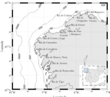
The Rías Baixas are constituted by four coastal embayments (>25 km3) on the western coast of Galicia (NW Spain), Ría de Muros and Noia, Ria de Arousa, Ría de Pontevedra and Ría de Vigo (Álvarez-Salgado et al., 1993) (Fig. 1.2), situated in the northernmost limit of the Eastern North Atlantic Upwelling System (ENAUS), a branch of the Canary Upwelling system (Alvarez et al., 2009). At the latitudes of the Rías Baixas, upwelling events result in the movement of Eastern North Atlantic Waters (ENAW), across the shelf coming into the Rías along the bottom (Fig. 1.3) (Álvarez-Salgado et al., 1993).

9

Figure 1.2: Location of the Rías Baixas.

Figure 1.3: Upwelling, NACW (North Atlantic Central Water) (Fraga, 1988).

At the Rías Baixas, upwelling occurs more frequently from April to September due to the predominance of northerly winds (Blanton et al., 1987). However, there are authors reporting longer upwelling periods, from March–April to September–October (Alvarez

et al., 2009). Coastal upwelling has also been observed even in autumn-winter under

some specific wind conditions as it occurred in January 1998, when there was pumping of seawater from the Iberian Poleward Current into the Ría de Pontevedra (Alvarez et

al., 2009). Upwelling/relaxation cycles as a result of these coastal winds occur with a

periodicity of 10 to 20 days during the upwelling season (Álvarez-Salgado et al., 2002). During winter, southerly winds appear forcing the coastal downwelling in the superficial waters, under the influence of the Iberian Poleward Current (Alvarez et al.,

10 2009). Furthermore, the run-off of the rivers contributes to the presence of river plumes over the shelf which varied rapidly according to wind stress (Cobo-Viveros et al., 2013). Part of the biomass produced in the Rías is exported to the shelf by these river plumes, and together with this downwelling front, the biomass will reach the bottom layer over the shelf where remineralization takes place. The downwelling will provoke homogenization of the water leaving the biomass in the bottom. Sometimes when there is less solar radiation, the biomass levels are low. In the frontal zone of the Ria where the proper dynamic of recirculation and sink zones of the Ria accumulates biomass, where the local gradient of salinity is higher (Álvarez-Salgado et al., 1993; (Nogueira et

al., 2000; Gago et al., 2003).

The intensity of the seasonal upwelling and downwelling in this region varies strongly between different years (Arístegui et al., 2006), describing decadal cycles linked to NAO (Hurrell, 1995).

This project will be focused in Ría de Vigo where winds are mainly responsible for the changes observed in the hydrography, and these changes are also associated with the two-layered residual circulation pattern which is characteristic of partially mixed estuaries (Diz et al., 2006). It is considered a partially mixed estuary because it is forced by wind stress as coastal upwelling systems and not by continental runoff as commonly found in mixed estuaries (Doval et al., 2016). The positive residual circulation is the inflow through the bottom layer and outflow through the surface layer, happening under the influence of northerly winds. When there is a reversal of winds, under southerlies the inflow will be through the surface layer and the outflow through the bottom layer (Diz et al., 2006).

The unique combination of wind patterns and coastal morphology makes the Rías Baixas a highly productive system, where frequent upwelling events occur, promoting an enrichment of nutrients and availability of CO2, an exceptional site for the extensive culture of the blue mussel Mytilus galloprovincialis. It represents one of the major shared world markets of blue mussels, with a total production of about 250,000 tons per year, representing 40% of European, and 15% of the world production (Álvarez-Salgado et al., 2008).

11 1.2.1 CO2 in the upwelling regions and at the Rías Baixas

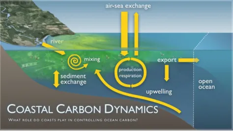
Under upwelling events, pCO2 supersaturated waters are brought to the surface to the coast of EBUS (Borges and Frankignoulle, 2001), playing an important role in the air-sea exchange of CO2 (Álvarez-Salgado et al., 2002). Nevertheless, these air-sea exchanges are particularly complex (Fig. 1.4), as a result from processes that have antagonistic effects on the surface seawater partial pressure of CO2 (pCO2) values (Borges and Frankignoulle, 2001; Borges et al., 2005). Several recent articles reporting global estuarine and coastal ocean CO2 fluxes concluded that although the global estuarine and coastal area is very small, this CO2 degassing flux is as large as the CO2 uptake by the continental shelf and that both flux terms are significant in the global CO2 flux (Cai, 2011).

Figure 1.4: CO2 cycle air-sea exchange (Team, 2018).

The great number of uncertainties to predict CO2 changes air-sea water exchange, in the role of the continental shelf seas depends on the availability of CO2 data in spatial and temporal scales (Cobo-Viveros et al., 2013). Although several studies have deal with the fCO2sw in surface waters in the coastal zone, there has been little emphasis on upwelling regions. As there, biological productivity can be very high, fCO2sw can be rapidly reduced (Gago et al., 2003). Some authors report that biological processes in

some places can be as important as changes in temperature (Simpson and Zrino, 1980). In general, the available data sets do not fully cover the annual cycle. So, it is unclear if upwelling systems behave as sinks or sources of atmospheric CO2 (Borges and Frankignoulle, 2002).

12 Studies agree that the NW Iberian upwelling system behaves as a sink for atmospheric CO2 (Pérez et al., 1999). The high absorption rates are due to the relatively low pCO2 levels of the upwelled waters, compared with aged central waters of the coastal upwelling regions that act as sources of CO2 to the atmosphere, and due to the intermittency of the NW Iberian upwelling. This fact allows for an efficient utilization of upwelled CO2 and nutrients that increase primary production, comparable with other coastal upwelling systems where the nutrient input is much higher (Arístegui et al., 2006).

1.3 CARBON DIOXIDE IN THE OCEAN AND AIR-SEA CO

EXCHANGE: CARBON MEASUREMENTS

The direct atmospheric measurements began 1958 by analyzing air enclosed in polar ice with ice core measurements (Etheridge et al., 1996). In recent years due to climate changes and the concern about the rise of CO2 levels, there is an urgency to study the CO2 seawater exchange.

The increase of atmospheric levels of CO2 accounts for about 60% of the CO2 emitted by fossil fuel sources (Wanninkhof et al., 2009). The seasonal cycle of CO2 atmospheric molar fraction (xCO2atm), is the result of a combination of uptake and release by plant and soils and seasonally by oceanic waters and anthropogenic emission (Padin et al., 2007). The gas exchange contributes to the migrations of the greenhouse anthropogenic gases through the absorption by the oceans of the excess of CO2 (Wanninkhof et al., 2009). The ocean uptakes CO2 from the atmosphere within the range of 17–39% of the fossil fuel emissions (Siegenthaler and Sarmiento, 1993).

In the water, there are different forms of carbon, the form the total dissolved inorganic carbon (Eq. 1):

(Equation 1)

The global mean total carbon in deep waters below 1200 m is higher than in surface mixed layers. So, it is important to understand how this carbon cycle works in between the ocean and the atmosphere (Legendre et al., 2015). The carbonate system is expressed in the following reactions (Eq. 2):

13 _{(Equation 2)}

The carbonate pump also creates a vertical gradient in total alkalinity (Eq. 3) (Legendre

et al., 2015):

(Equation 3)

Total alkalinity (AT) is a measure of the capacity of the water to neutralize hydrogen ions, balancing the electric charges in seawater. AT is a quasi-conservative parameter, which can be influenced only by the massive proliferation of calcareous microalgae. The vertical variability of the chemical carbon pump is important because is one of the driving factors for the exchange of CO2 seawater- atmosphere and drives CO2 to the depth ocean (Legendre et al., 2015).

The magnitude of the ocean carbon sink depends on several competing effects in the CO2 partial pressure differences across the air-sea interfaces due to differences in temperature. Seawater warming reduces solubility and increases pCO2 in the mixed layer. When the seawater is colder, solubility in the water increase while when the temperature in the seawater is warmer, the solubility for the CO2 in the water is reduced. The accumulation of CO2 in the ocean decreases pH and shifts carbonate chemistry to high dissolved CO2 gas fractions (Fung et al, 2005).

To determine the CO2 difference between the surface waters and the atmosphere, it is necessary to evaluate the fugacity of CO2 in seawater (fCO2sw) and in the atmosphere (fCO2atm). The fugacity of CO2 is related to partial pressure, but it is not exactly the same since it is the product of the mole fraction (xCO2atm) times the total pressure. Fugacity takes into account the non-ideal nature of the gas phase (Dickson et al., 2007), rather than considering it as an ideal one. The difference between pCO2 and fCO2 can be usually assumed a 0.3%, a procedure sufficient accurate for the purpose of air-sea CO2 (Lewis, 1998).

The interannual variations in the atmospheric forcing in response to modes of climatic variability and other physical and biological processes in the upper ocean, like upwelling, should play an important role in the determination of the interannual

14 variability of the CO2 uptake in the global ocean (Borges and Frankignoulle, 2001; Olsen et al., 2003).

1.4 BAKUN'S THEORY

Climate change is one of the most important challenges in our time. It is a change produced on a global scale but with effects in local terms and in different science fields. For example, in 2015 the average increase in temperature across global land and ocean surfaces was 0.9°C, and this was the highest among the overall 136 years of records from the Department of Commerce (2018) while the year before was only 0.16°C. One of the issues of this change will be the differences in the wind stress due to the differences in temperature caused by the greenhouse gasses accumulated in the atmosphere. So this challenge of climate change is changing the pattern of EBUS. The problem is to understand how global change is affecting these systems.

Within this approach, Bakun (1990) published a theory about this issue titled "Global Climate Change and Intensification of Coastal Ocean Up-Welling". This article was referring to an apparent paradox associated with the idea that global warming might lead to an intensified cooling of local areas affected by coastal upwelling (Barton et al., 2013).

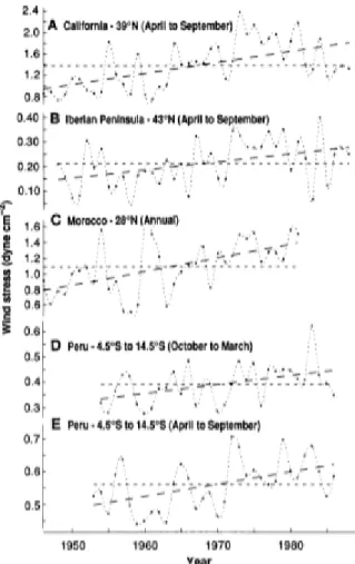
The theory is based on the substantial increase of CO2 and other greenhouse gases in the atmosphere (IPCC, 2018), which will create an inhibition of cooling in the night that will develop a heating intensification in the continental zone adjacent to upwelling regions. For this author, the alongshore wind that drives coastal upwelling will be maintained in part by a strong atmospheric pressure gradient developed over the heated land mass and the higher barometric pressure over the cooler ocean (Bakun, 1990), rising wind stress that, will increase the intensity of the upwelling (Bakun and Weeks, 2004). For example, in the case of Iberian Peninsula, like in California, Bakun (1990) indicated an increase in the northeastern Atlantic Ocean wind stress during the spring to summer upwelling season between the 1950s and 1980s (Fig. 1.5). Nevertheless, the IPCC reports state that this "global warming" should not always lead an increase in the local temperatures.

15

Figure 1.5: Year averages of monthly estimates of alongshore wind stress of California, Iberian Peninsula, Morocco, and Peru. Short dashes indicate the long-term mean of each series while

longer dashes indicate the linear trend fitted by the method of least squares (Bakun, 1990).

In consequence, there are several scientists trying to test this theory in different locals of the planet. For example, data of significant cooling of surface waters from the coastal upwelling area off Cape Ghir (North West Africa near 30.5°N) during the latter part of the 20th century (Lemos and Pires, 2004) were reanalyzed by McGregor et al., (2007), and support the “Bakun hypothesis”, while a decrease in coastal upwelling intensity of the coast of Portugal in the later part of the 20th century was observed (Narayan et al., 2010). As stated by Relvas et al., (2009) there is a time lag between the different projects and scales about how is changing the SST and Wind Stress, (microscale in the order of 10 m, mesoscale in the order of 50 km or macroscale in the order of >1000 km) that will conduct to a different conclusion regarding the increase or decrease of upwelling intensity. It is perceived by some scientists a warming-up trend in the Eastern North Atlantic and in the coastal regions (Relvas et al., 2009), which is in opposition to Bakun's hypothesis.

16 One variable that Bakun did not take into account was the North Atlantic Oscillation (NAO), which is an index based on the surface sea level pressure differences between the Subtropical Azores high cell and the subpolar low cell (Ncdc.noaa.gov, 2018). During a positive NAO, conditions are colder and drier than average over the northwestern Atlantic and Mediterranean regions, whereas conditions are warmer and wetter than average in Northern Europe, the Eastern of the United States and part of Scandinavia (Visbeck et al., 2001). NAO is widely recognized as the most significant pattern of climate variability in the North Atlantic sector (Visbeck et al., 2003) and it has shown modes that may lead simultaneously local warmer or cooler effects (Perez et

al., 2010). It has been recognized too, that the fluctuations in SST and the strength of

the NAO, are related, and there are clear indications that NAO varies significantly with the overlying atmosphere, and hence, it is possible that anthropogenic climate change might influence the natural variability of the NAO.

1.4.1 Bakun's theory application at the Rías Baixas

At the Rias Baixas on the Galician coast of Spain, despite the increase of winds for the Iberian Peninsula, there is a general weakening in upwelling intensity. There is an overall warming observed in the Iberian/Canary current region, that exceeds the mean oceanic values (Pardo et al., 2011), as reported by other authors, such as Sydeman et al., (2014) that reworked quantitatively data of wind trends information data from 22 studies published between 1990-2012. These data were used to test if the winds were increasing (consistent with Bakun's theory) or decreasing (inconsistent with Bakun's theory). The data provided and tested, support the hypothesis of wind intensification in the California and Humbolt systems, whereas the Iberian system was inconsistent with Bakun's hypothesis, by winds weakening. The authors concluded that the annual average wind trends did not support the upwelling intensification hypothesis (Sydeman

et al., 2014). Relvas et al. (2009), using Sea Surface Temperature (SST) by satellite

imagery, got a generalized warming trend in the coastal waters of the Western Iberian Peninsula for the period 1985-2003.

17

1.5 OBJECTIVES

Taking into account the Bakun theory application for the Rias Baixas, this thesis has as a major objective to estimate the annual CO2 fluxes and upwelling in Galicia between 1997 and 2017. This work is important given the difficulty to monitor variables such as temperature, salinity, pH, in long-term scenarios provided by instrumentation, and the difficulty in taking measurements at sea (Casey and Cornillon, 2001).

To achieve this, specific objectives will be developed:

- To analyze the chemical changes associated with the large-scale variability of upwelling systems (CO2 fluxes), physical variations in terms of upwelling and thermohaline, and biological forcings such as chlorophyll an (as a proxy of phytoplankton development) and net ecosystem production.

- Furthermore, it will be analyzed the long-term impact of CO2 fluxes on primary production in the Galician coast.

18

2. VARIABLES TO CALCULATE AIR-SEA CO

FLUX

AND UPWELLING INDEX

2.1 AIR-SEA CO

FLUX

There are many variables that can affect the calculations of the air-sea CO2 flux (FCO2) (Fig.2.1) The measurements of fugacity require normally, a gas phase balanced with sea water knowing pressure and temperature (Dickson et al., 2007). Nowadays, the major uncertainty in the calculation is attributed to the estimation of k (gas transfer velocity) parameter (Takahashi et al., 2009).

Figure 2.1: Variables that can affect the calculation of air-sea CO2 flux, on the left, environmental

forcing factors, on the right the factors that can affect the air-sea pCO2 gradient (Wanninkhof et al., 2009).

This is parameterized as a function of the wind speed that is the main factor to relate to the gas transfer (Wanninkhof et al., 2009). The dependency differs a lot among studies, and it has been stated as linear, kL&M (Liss and Merlivat, 1986) (Eq. 4), quadratic kW, kN, ks computed by Wanninkhof, 1992; Nightingale et al., 2000; Sweeney et al., 2007, respectively (Eq. 5, 6, 7), and cubic, kM&G, (McGillis et al., 2001; Eq. 8) where Sc refers to the Schmidt number and U10 refers to the wind speed; a, b and c are coefficients dependent on the wind speed and 600 and 660 are the Sc values in fresh water or sea water respectively, at 20ºC of temperature. Other physical processes affect the estimation of this constant, such as thermal stability, the presence of surface surfactants or rainfall. Due to the non-consensus with respect to the best k parameterization, it is

19 important to give special attention to the quality of the wind speed data, particularly using quadratic and cubic parameterizations. The sources can be different. The data taken from ships can be distorted due to the structure of the ship, which gives a bias in the data. It is possible to take the data from buoys too, but they are not totally consistent with the locations and time of the measurements of ΔpCO2. Finally, model data and data from Satellites such as QuickSAT, Seawinds or SSM/I, are the best ones due to their homogeneity and quality in large spaces, with a high resolution (0.25º) (Otero et al., 2013; Remss.com, 2018)). (Equation 4) (Equation 5) (Equation 6) (Equation 7) (Equation 8)

xCO2atm seems not being a critical variable for the estimation of air-sea CO2 fluxes. This is due to, the fact that in the high atmosphere the ratios in the mixing keep a seasonal variability of the CO2 atmospheric molar fraction (xCO2atm) smaller than in sea-water (Padin et al., 2007).

The interest in gas fluxes in the ocean is related to a phenomenon happening at different temporal and spatial scales. To achieve the air-sea CO2 flux, it is required to understand the influence of these factors (Fig.2.1) in the CO2 flux. By convention, if a flux is negative means that the ocean is acting as a sink, while when the flux is positive, the ocean is acting as a source (Wanninkhof et al., 2009).

Upwelling phenomenon in coastal waters is an important process to take into account in the study of air-sea CO2 flux. Upwelling brings to the surface, colder waters from the bottom, enriched in gasses like CO2, both the changes in temperature an enrichment of CO2 in surface waters provoke changes in the air-sea CO2 flux.

20

2.2 UPWELLING INDEX DERIVED FROM BAKUN THEORY

The upwelling index used in this project is based on Ekman Transport and it is more appropriate for evaluating temporal variations of upwelling intensity (Lamont et al., 2017). Eq. 9 can be worth for purposes such as determining potential biophysical effects of anthropogenic global warming (García-Reyes et al., 2014).

(Equation 9)

Where ρair is the density of the air (1.22 kg m-3 at 15°C), ρsw is the density of the seawater (~ 1025 kg m-3), f is the Coriolis parameter (9.946·10-5 s-1 at 43°N), y is Shelf wind stress, CD is an empirical dimensionless drag coefficient (1.4·10-3 according to Hidy, 1972), V and Vy are the average daily strength and a northerly component of the wind, respectively.

The upwelling index represents the offshore Ekman transport value but with a different sign. It will be positive when the Ekman transport is offshore and upwelling favorable (Herrera et al., 2005).

There is a possibility SST-based index which provides a good representation of the spatial variation of upwelling (Lamont et al., 2017). Nevertheless, the one derived by Bakun, (1973) (Eq. 9) was the one chosen for this project and it has been chosen for decades. The formula is an estimation of the cross-shelf Ekman transport due to geostrophic wind stress calculated from large-scale atmospheric pressure gradients (García-Reyes et al., 2014).

To measure the upwelling index there are another ways, for example in coastal zones upwelling is driven by a cyclonic curl of wind stress, this cyclonic curl is one order of magnitude lower than Ekman transport (Lamont et al., 2017).

21

3. MATERIAL AND METHODS

3.1 STUDY AREA

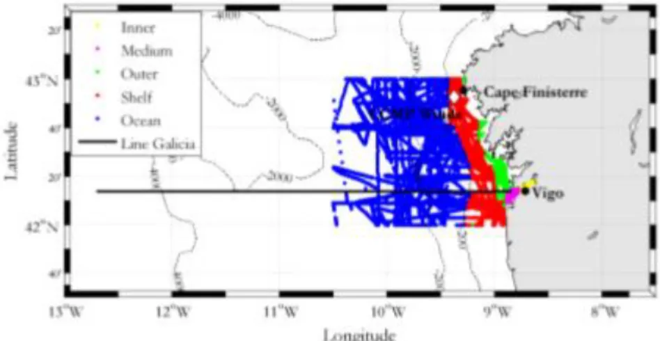
The study area where pCO2 data were taken corresponds to a large coastal embayment close to Vigo (Gago et al., 2003) as shown in Fig. 3.1. These data derived from several oceanographic cruises made by the Marine Research Institute belonging to the Spanish National Research Council (IIM-CSIC) in Vigo (Spain). The final database used to cover the area from 42°N to 43°N and from coast to 10.5°W, the longitude that marks the eastern boundary of the Iberian Current (Alvarez et al., 2009). The ria was divided

into Inner, Middle and Outer zones following the same pattern as described by Gago et

al., (2003).

Figure 3.1: Map of the Galician rías, continental shelf, and ocean, showing the five studied zones: “Inner” (data from 8.64ºW to 8.78ºW, yellow) and “Middle” (8.78ºW to 8.9ºW, magenta); “Outer” for the data measured outside the Ría de Vigo from 8.9ºW until 50 m depth (green); "Shelf" for the data measured between 50-200 m depth (red); and "Ocean" for data measured from 200 m depths

until 10.5ºW (blue).

3.2 OCEANOGRAPHIC CRUISES

Working data were taken from different oceanographic cruises embedded in different projects such as, Dynamics and Biogeochemical short-scale variability in the Galician continental shelf – DYBAGA; Evolution of CO2 increase using ships of Opportunity: Galicia and Bay of Biscay – ECO; CUBE; Community Structure, Trophic Functioning, and Biogeochemical Plankton Rates during downwelling in the Coastal Transition Zone

22 of NW Spain – ZOTRACOS; and Reactivity of Dissolved Organic Matter in the upwelling system of the Ría de Vigo – REMODA, NAVAZ and finally the one that is actually running ARIOS (Acidificación en las Rías y Plataforma oceánica ibérica). The data that were not possible to take from these oceanographic cruises, were taken from SOCAT which are data from other Oceanographic campaigns of other National Research Institutes.

ARIOS project is explained in detail since there was a personal participation on it to learn each step. The data were processed from the beginning with raw data for 2017 and 2018, while the rest of the data were in another state of processing or downloaded from a database.

For ARIOS project, samples were taken in 9 stations along the transect (Fig.3.2, Table 1.1). The stations in the outer part of the Ria were 1, 2, 3, 4 and 5 while inside were 6, 7, 8 and 9. In each station was thrown a rosette with 12 Niskin bottles (Fig.3.3). The samples were taken thinking in the exchange of gases, being the oxygen the first one to be sampled, using a thermometer to determine a constant temperature using the Winkler method (Winkler, 1888). Secondly, the cuvettes for pH were sampled. Next, it was taken samples for determination of alkalinity, nutrients, and salinity. For all the samples it was important to take the samples without bubbles. Finally, it was taken the samples for chlorophyll, with a volume of 250 mL using a test tube which was filtered in the ship and the filters were kept in a freezer in tubes wrapped in aluminum foil to avoid to degradation of the chlorophyll until further analysis in the laboratory.

Figure 3.2: Stations along the coastal zone and ocean interior where samples are taken in ARIOS campaigns.

23

Table 1.1

ST in the show the locations from the map. The number of levels where there were taken samples, Zmax, is the maximum depth where there were taken samples.

ST Lat (ºN) Lon (ºW) Nº Levels Z MAX

1 42º 7.980' 9º 30.000' 11 200 1.1 42º 7.980' 9º23.352' CTD 200 1.2 42º 7.980' 9º16.686' CTD 200 2 42º 7.980' 9º 10.020 10 150 3 42º 7.980' 9º 3.000' 9 125 4 42º 7.980' 8º 56.760' 7 80 5 42º 9.720' 8º 53.520' 6 50 6 42º 14.820' 8º 53.100' 4 22 7 42º 14.400' 8º 45.720' 5 40 8 42º 16.200' 8º 42.120' 5 22 9 42º 17.520' 8º 39.120' 3 20

24 In order to improve the characterization of the section, there were done two stations 1.1 and 1.2 (Fig. 3.2), in which, it was thrown a CTD and a Fluorometer Turner. Inside the ship, there were continuously measurements along the whole campaign of dissolved oxygen with an Optode (Aanderaa), of pH with an AFT Sunburst and chlorophyll a with a fluorometer (SeaFet). The pH measurements were afterward used to calculate the pCO2 in water.

3.3 DATA TREATMENT

Salinity samples were collected in all stations at selected depths to calibrate the conductivity sensor installed in the CTD bathysonde and in the underway thermosalinograph. Samples were stored for 24 hours in the laboratory under controlled temperature (22ºC) before analysis (Fig. 3.4a). During the first leg of the cruise, salinity samples were collected in all stations at 3 selected depths (two in deep water and one in the surface) and were analyzed using PORTASAL Guideline and calibrated with one only existing IAPSO standard seawater. A container of 50 liters was filled with seawater collected at 2500 meters depth at station 5. This water was used during the cruise as a substandard during the cruise and was analyzed at the beginning and at the end of each series of analysis to check the drift of the PORTASAL.

During the same day of the cruises, it was important to start the measurements of seawater pH samples which were taken at 24 levels in all the stations along the FICARAM-XVII section. pH measurements were made using the spectrophotometric method described in Clayton and Byrne, (1993). This method consists of adding 75 µL of m-cresol purple (mCP) to the seawater sample and measuring its absorbance at 3 wavelengths, i.e., λHI =434 nm; λI =578 nm and λnon-abs=730 nm (Fig. 3.4b). The reaction of interest at seawater pH is the second dissociation (Eq. 10) in which I is the indicator. Then, the total hydrogen ion concentration can be determined by Eq. 11. pH samples were taken directly from the Niskin bottles into special optical glass spectrophotometric cells of 28 mL of volume and 100 mm of path length. These cells were carefully stored in a thermostatic bath at 25.0ºC around one hour before the analysis. Absorbance measurements were performed with a Perkin Elmer Lambda 850 UV-VIS spectrophotometer on board the R/V Hespérides. pH values were given following the

25 equations described in Dickson et al. 2007, who includes a correction due to the difference between seawater and the acidity indicator (ΔR).

HI−(aq)=H+(aq)+I2−(aq) (Equation 10) pH=pK2+log10[I2-]/[HI-] (Equation 11)

After this, during the next day, it was measured the samples of AT which were taken during the FICARAM section every each station, almost half of the total stations. In order to analyze these AT samples on board, the water was transferred directly from the Niskin bottle to 600 mL borosilicate glass bottles and stored for 24 hours before the analyses. Measurements of AT were done by a one endpoint method using an automatic potentiometric titrator (Dosino 800 Metrohm) with a combined glass electrode (Fig. 3.4c). A Knudsen pipette (~195 mL) was used to transfer the samples into an open Erlenmeyer flask in which the potentiometric titration was carried out with HCl (0.1 M). The final volume of titration was determined by means of one pH endpoint (Körtzinger

et al., 1996). In order to estimate the accuracy of the AT method, AT measurements of certified reference material (CRM) for CO2 from batch 100 provided by Dr. Andrew Dickson was analyzed. In addition, an extra calibration (substandard) was made by using a closed container of 75 L filled with open ocean surface water.

26

Figure 3.4: (a) the salinometer, (b) spectrophotometer to measure pH, (c) titration apparatus to measure alkalinity.

For this project, pH was measured continuously as well as other parameters such as sea surface temperature (SST), sea surface salinity (SSS) which gave the data to calculate alkalinity, to determine pCO2sw. However, it was important to take samples and analyze them in the laboratory. Using this procedure it was possible to correct the measurement done in continuous. Measurements done in the laboratory are more reliable than the ones taken with a sensor.

3.4 ESTIMATION OF CO

AIR-SEA EXCHANGE

3.4.1 Data script preparation: fCO2sw calculations

First of all, it was necessary to determine the Alkalinity. With alkalinity data from the laboratory, it was determined a regression line with data of a whole year for the surface values of both SSS and Alkalinity. With these linear equations, it was determined the alkalinity from the continuous data of SSS (Eq. 12). Eq. 12 is an example for the years 2017 and 2018 for the ARIOS project, where y=Alkalinity and x=SSS.

27 Equation 12

R2 = 0.80

With pH, it was done the same procedure using the data measured in the laboratory and making the linear equations with the data registered with the AFT Sunburst for each campaign, matching the data where there were values of both measurements. Then pH was corrected using again the linear equation. After these calculations, for the pH corrected it was done a running mean to determine an average value of the data using MATLAB software as we can see in the example in Fig. 3.5.

Figure 3.5: Running mean in blue and raw data in red, from the pH data corrected, this data are from 2017 and 2018.

Knowing both pH and Alkalinity it was possible to calculate pCO2sw. This calculation was done from the campaigns explained before, between 1997 and 2018, to better understand the long-term variability since there were some gaps in the data set. When there were not campaigns data were attained from SOCAT where data from other Oceanographic campaigns of other National Institutes Research exist. The transformation of pCO2 into fCO2 was done through the difference between them which is lower than 0.3% (Weiss, 1974; Olsen et al., 2003).

28 3.4.2 Data script preparation: fCO2atm calculations

The data of atmospheric CO2 fugacity was estimated from the monthly values of atmospheric CO2 molar fraction recorded in meteorological stations of the NOAA/ESRL Global Monitoring Division stations, Mace Head (mhd) and Izaña (Izo) (Fig. 3.6). The xCO2atm were linearly interpolated versus latitude for the calculations of CO2atm, while the final xCO2atm dataset was converted to atmospheric CO2 partial pressure (pCO2atm) (Eq. 13). With this aim, first, to calculate the water vapor pressure (pH2O) it was used the formula from Weiss and Price (1980), where S and T were salinity and temperature (ºC) (Eq. 14). The final xCO2atm dataset was converted to pCO2atm, considering Patm and pH2O (in atm), which was calculated from in situ SST readings (Eq. 13) (Weiss, 1974). The pCO2 values were then converted to fCO2atm assuming a decrease of 0.3% from the pCO2atm value (Weiss,1974), due to the non-ideal behavior of carbon dioxide (Gago et al., 2003).

Figure 3.6: Izaña is the purple point situated in the Canary Islands, Mace Head is the green point situated in Irland both forming a triangle with the zone of this project in Galicia, redpoint.

The more recent data out of a period that covers the data series for both stations between 2010 and 2017, were estimated extending the seasonal variation from the interannual tendency observed from 2010 to 2017, until 2018.

To calculate the water vapor pressure (pH2O) that enters in the calculation of the pCO2atm it was used the formula from Weiss and Price (1980), where S and T were salinity and temperature (ºC) (Eq. 14). The final xCO2atm dataset was converted to

29 pCO2atm, considering Patm and pH2O (in atm), which was calculated from in situ SST readings (Eq. 14) (Weiss, 1974).

pCO2atm = xCO2atm (Patm pH2O) (Equation 13) pH2O (S,T)

(Equation 14)

3.4.3 Data script preparation: FCO2 Flux calculations

The CO2 exchange between the ocean and the atmosphere (FCO2, in mol m−2 yr−1) was calculated by Eq. 15, where K was the CO2 gas transfer velocity (cm h-1, estimated from wind speed), S was the solubility of the CO2 in the seawater estimated according to Weiss, 1974 and ΔpCO2 was the difference between pCO2sw and pCO2atm. A negative flux means that the ocean was absorbing atmospheric CO2 while a positive flux means that the ocean was emitting CO2 into the atmosphere.

(Equation 15)

K parameter, as it was explained before, is a crucial parameter that depends mainly on

the quality of the wind speed data that was calculated using the Cross-Calibrated Multi-Platform (CCMP) (Remote Sensing Systems, 2018) which is a remote sensing system. 3.4.4 Complementary data sources

3.4.4.1 NEP data

Net Ecosystem Production (NEP) was included in the dataset as a proxy for photosynthetic activity (Science.oregonstate.edu, 2018). It was obtained by the Vertically Generalized Production Model (VGPM) (Behrenfeld and Falkowski 1997) that is fed by Chl a, SST, and photosynthetically active radiation (PAR) information as inputs, which was obtained from Sea-viewing Wide Field of view Sensor (SeaWiFS) and Moderate Resolution Imaging Spectroradiometer (MODIS) Sensor. It was downloaded and interpolated using "nearest-neighbor" since the data was taken from a transversal line which included all zones, from -8.64ºW to -13ºW in the latitude 42.2ºN. Afterward, it was calculated the average for each month.

30 3.4.4.2 Wind speed, chlorophyll, and NAO data source

In order to make the calculations of upwelling index (Eq. 9), it was used data of Wind speed and SST which was obtained from (NCEP/NCAR Reanalysis I). In this case, it was decided to use this SST data and not the continuous data because of the scale of upwelling is much bigger and the continuous data measured in-situ could give larger errors while drawing conclusions.

Chlorophyll was taken from, SeaWiFS between 1997 and 2010 with a 9 km resolution, and from MODIS between 2011 and 2018 with a 4 km resolution (Oceandata.sci.gsfc.nasa.gov, 2018). These data of Chla, were important to make the correlation with the NAO index. Finally, monthly data of NAO Index was taken from "Climate Prediction Center - Teleconnections: North Atlantic Oscillation", (2018).

3.5 BIOCHEMICAL FORCINGS

3.5.1 fCO2sw variability between biological and temperature components

For both Eq. 16 and 17 SSTmean is the annual average in ºC, and SST is sea surface temperature observed in ºC. fCO2sw is the data observed in atm (Eq.16) while fCO2swmean is the annual average of the fCO2sw observed (Eq. 17). Both formulas were used to explore how much the final fCO2sw data (Takahashi et al., 2002) is affecting the thermodynamic component and the biological component.

(Equation 16) (Equation 17) 3.5.2 Seasonality of the variables

Eq. 18 was done to model the variability of the fCO2 considering its drivers: SST, SSS, and Chla). Simultaneously, it includes the seasonal cycle to model the temporal variation, being the seasonal cycle of major importance than its drivers. For the seasonal cyclicity, it was used 4 harmonics with a period of 12, 6, 4, and 3 months.

The SST had a special treatment, by calculating the SST anomalies, which were the values above or below the average SST in each moment. When SST anomalies were positive, the saturation of fCO2sw increases as it was expected, and when SST anomalies

31 were negative, these should diminish the saturation of fCO2sw. However this does not happen because when there is a negative SST anomaly, that can be upwelling, the waters are rich in dissolved gases as CO2. For this reason, it is important to test both SST anomalies split in SST>0 and SST<0.

(18) 3.5.3 Statistical Analysis

The normality of the different variables was checked by using Software SPSS with a test of Kolmogorov-Smirnov. It was added two new variables apart from SST, SSS, Chla, ΔfCO2, FCO2 and Iw, which were NAO Index taken from Department of Commerce-NOAA, (2018) and Winter NAO Index which was a group of data done when the differences of the NAO Index are higher as during December, January, and February. Using monthly averaged for all the variables, the data was split into two groups, Ria and Off-shore. Because the Kolmogorov-Smirnov test was normal, it was elected a Pearson correlation to determine the relationship between variables. This was done with the aim of observing if there is some relationship between the studied variables between 1997 and 2018 and the NAO.

32

4. PRECEDING RESULTS

Figure 4.1 shows the data since 2010 of levels of xCO2 in the atmosphere. This was an important parameter to determine the CO2 flux difference between seawater and atmosphere. There is a tendency to increase each year, having seasonal variation in the same proportion every year. This was one of the important parameters to support Bakun's theory of Wind Stress diminishing.

Figure 4.1: Data downloaded from xCO2, 2018 is an estimation from the past years.

Figure 4.2 has two important variables to calculate fCO2sw, Fig.4.2a is the pH that remains constant during 2017 and 2018. Alkalinity has the same constant behavior which is important when determining fCO2sw. Alkalinity (Fig.4.2b) acts as a tampon which is the capacity to maintain a stable pH along time. Both together can allow the calculation of pCO2 contained in the sea-water at a certain time.

33

Figure 4.2: (a) Daily average of pH taken over the cruises in continuous, between 2017 and 2018 embedded in the ARIOS project. (b) data of specific alkalinity calculated from SSS data taken in

34

5. RESULTS

5.1 DATA AVAILABLE FOR THIS PROJECT

As it is possible to observe in Fig. 5.1, there are years with no data available, and that there is not the same amount of data for the different zones, which is important and an issue to have in account when discussing the results and drawing conclusions. The Ría de Vigo, represented by the Inner, Middle and Outer zones, have less data, in opposition to off-shore represented by Shelf and Ocean. There is a gap of data between 2006 and 2008 for the overall zones. The colors presented for the different zones will be the same

ones for the rest of the project.

Figure 5.1: Data available for this project for the different zones.

5.2 SEASONAL VARIABILITY

5.2.1 Seasonal variability of SST, SSS, FCO2, ΔfCO2, and NEP

As can be observed in Figs.5.2 and 5.3, SST maintained consistently the seasonal variability in the 5 zones, with higher values in summer and lower during winter, as expected. During the summer it is observed a decrease of temperature in August for all the zones, less pronounced in the middle zone. In all the cases, the maximum values of SST coincided both before and after the peak of the upwelling period. During Summer, when the solar radiation is higher it was achieved a maximum SST for the whole area in

35 the Ocean zone of 20.2 ºC on September (18.81.4 ºC, Table 5.1) when the occurrence of upwelling is decreasing (Fig. 5.4).

Minimum SST in all over the area are achieved during winter season, but there is a clear difference between the Inner and Middle zones, in January (12.2 ºC and 12.1 ºC respectively, Table 5.1), and the Outer, Shelf, and Ocean zones (12.6 ºC, 12.9 ºC, and 13.1 ºC respectively, Table 5.1), in March.

The highest differences in a month (referring to the SD) of SST was found during Summer when there is the major upwelling prevalence (Fig. 5.4). Upwelling brings colder waters from the bottom to the sea surface waters and changes drastically the temperature during this season. The lowest monthly SD between SST was recorded during the Winter months when there is downwelling.

In the case of SSS, this variable is relatively homogeneous in the Ocean with a maximum SD of 0.24 during July (Table 5.1). The Outer and Shelf zones behave like transition zones where the maximum SDs were recorded during the winter season, 0.95 and 1.13, in March and January respectively (Table 5.1). In the case of Inner and Middle zones, since these zones are the nearest to the continental run-off of fresh water, the variability of salinity is maximum, with the highest SD of 3.69 and 1.51 found in December and January respectively (Table 5.1). In the case of the Inner zone, salinity decreased to values lower than 30 during December (Table 5.1 and Fig. 5.2).

ΔfCO2,which is the difference between fCO2sw and fCO2atm, is the capacity of absorbing more or less fCO2 by the sea water. If the value is negative, then there is the capacity to absorb more but if it is positive then, the seawater cannot absorb more CO2. Because the fCO2sw depends on many variables such as SST, the SD of ΔfCO2 in each moment can change rapidly. This is the reason why the SD has a higher range in Table 5.1 than SST and SSS variables (Table 5.1).

The maximum values of ΔfCO2 inside the Ria correspond to October (Figs. 5.2 and 5.3). The Inner zone is where the maximum positive value of 194 µatm was achieved, showing an inverse behavior with respect to salinity. In the Off-shore the values are much less positive with a maximum of 2 µatm in the Shelf (Table 5.1) and -1 µatm in the Ocean (Table 5.1), both in November and September respectively. The minimum values were achieved inside the Ria during May in the Inner and Outer zones (Fig. 5.2)