Agrometeorology |
Article
modeling of extreme minimum air temperature
series of Campinas, state of São Paulo, Brazil
Gabriel Constantino Blain (*)
Instituto Agronômico, Centro de Ecofisiologia e Biofísica, Caixa Postal 28, 13012-970 Campinas (SP), Brasil. (*) Corresponding author: [email protected]
Received: February 9, 2011; Accepted: July 20, 2011
Abstract
Under the hypothesis that the presence of climate trends in the annual extreme minimum air temperature series of Campinas (Tminabs; 1891-2010; 22º54’S; 47º05’W; 669 m) may no longer be neglected, the aim of the work was to describe the proba-bilistic structure of this series based on the general extreme value distribution (GEV) with parameters estimated as a function of a time covariate. The results obtained by applying the likelihood ratio test and the percentil-percentil and quantil-quantil plots, have indicated that the use of a time-dependent model provides a feasible description of the process under evaluation. In this non-stationary GEV model the parameters of location and scale were expressed as time-dependent functions. The
shape parameter remained constant. It was also verified that although this non-stationary model has indicated an average
increase in the values of the analyzed data, it does not allow us to conclude that the region of Campinas is now free from frost occurrence since this same model also reveals an increasing trend in the dispersions of the variable under evaluation.
However, since the parameters of location and scale of this probabilistic model are significantly conditioned on time, the
presence of climate trends in the analyzed time series is proven.
Key words: extreme value, non-stationary, time-dependent functions.
Incorporando tendências climáticas na modelagem estocástica da série de
temperatura do ar mínima absoluta de Campinas, Estado de São Paulo
Resumo
Sob a hipótese de que a presença de tendências climáticas na série anual de temperatura do ar mínima absoluta de Cam-pinas, Estado de São Paulo (Tminabs; 1891-2010; 22º54’S; 47º05’W; 669 m), não pode mais ser negligenciada, o objetivo do trabalho foi descrever a estrutura probabilística com base na distribuição geral dos valores extremos (GEV), e parâmetros estimados em função da covariável tempo. Os resultados observados após a aplicação dos testes de Mann-Kendall, razão
da verossimilhança e gráficos percentil-percentil e quantil-quantil, indicaram que a utilização de um modelo dependente
do tempo resulta em uma descrição verossímil do processo sob avaliação. Neste modelo não estacionário, os parâmetros de localização e escala foram expressos como funções do tempo. O parâmetro de forma ou calda permaneceu constante. Observou-se também que embora o modelo tenha indicado aumento médio nos valores de Tminabs, não é possível concluir que a região de Campinas está atualmente livre da ocorrência de geadas, uma vez que o modelo também revela a tendência de elevação na dispersão dos dados da variável sob análise. Contudo, uma vez que os parâmetros de localização e de escala
são significativamente condicionados no tempo, a presença de tendência climática, na referida série, está comprovada.
1. IntroductIon
Statistical evaluations applied to meteorological time se-ries have been used to improve the capability of the human society in dealing with the influence of the climate vari-ability in almost all human activities. For instance, based on the relationship between agricultural production and air temperature values observed during the crop seasons, several studies have evaluated the probability of occur-rence associated with extreme minimum air temperature values in order to provide important information related to frosts(1) mitigations procedures (Camargo et al., 1993; Astholpo et al., 2004; Blain and Lulu, 2011).
Based on the Extreme Value Theory (EVT), Camargo et al. (1993) and Astolpho et al. (2004) used a particular case of the general extreme value distribution (GEV) - called Gumbel or Fisher-Tippet I - to describe the proba-bilistic structure of the annual extreme minimum air temperature series (Tminabs) available from the weather station of Campinas (hereafter referred just as Campinas). This time series is composed by the lowest air temperature value observed during each year.
Considering that the GEV has all the flexibility of its three particular cases (type I – Gumbel; type II – Fréchet and, type III – Weibull; Nadarajah and Choi, 2007), Blain and Lulu (2011) used the GEV distribution to assess the probability of occurrence associated with Tminabs values (1948-2007) ob-served in six regions of the State of São Paulo.
According to Leadbetter et al. (1983) and Wilks (2006) a basic assumption from the EVT is that the dis-tribution of the maximums of independent and identical-ly distributed (iid) random variables, converge to one of the particular cases of the GEV. This assumption is called the Extremal Types Theorem. Thus, the probability of oc-currence of an extreme event observed in any t year (xt) can be described as Pr{X ≤ xt}=GEV(xt; μ, σ, ξ); where
μ, σ, ξ are, respectively, the parameters of location, scale and, shape. Also according to Wilks (2006), although the EVT is often related to the description of the behavior of the maximum values observed in a data sample, its ap-proach is equally applicable to the evaluation of the small-est values observed in this data sample. In this case it is only necessary to transforming the variables x into –x and, consequently, –μ into μ.
It is worth emphasizing that the use of the GEV(xt; μ, σ, ξ) model is frequently called “the stationary approach” (Coles, 2001; El Adlouni et al., 2007; Pujol et al., 2007; Méndez, 2007; Furió and Meneu, 2011) since the probability associated with any xt is independent of t. In other words, once the GEV(xt; μ, σ, ξ) model is fitted from a (already) observed time series (for e.g. from the 1891-2010 time span) it is assumed that the values of
μ, σ, ξ will remain the same during the next (t) years (for e.g. 2011 to 2050). However, the Intergovernmental Panel on Climate Change (Ipcc 2001 and 2007) indicates that the intensity and the frequency of extreme events (such as extreme low air temperatures) will change due to the global warming. Furthermore, the Ipcc (2007) also states that the recent increases of the global air temperature already have perceptible impacts on many natural systems.
As indicated by Blain et al. (2009) the evaluation of the average annual minimum air temperature (Tmin) of Campinas seems to agree with this last statement of the IPCC (2007) since this time series has shown remarkable increasing trends during the last years. Indeed, consider-ing the years between 1890 and 2007, this annual series has shown a linear increasing trend at the rate of (approxi-mately) 2.5 ºC per 100 years (Blain et al., 2009).
These last considerations have allowed us to (i) work un-der the hypothesis that the use of a stationary GEV model may no longer be valid since the presence of climate trends in the Tminabs series of Campinas must not be neglected, and to (ii) assume that the development of a time-dependent model may provide a more feasible description of future re-alizations of the variable under evaluation. Thus, the aim of the work was to describe the probabilistic structure of the Tminabs data sample based on a GEV model in which the parameters are estimated as a function of a time covariate.
2. MaterIal and Methods
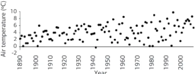
Annual extreme daily minimum air temperature data were used from the weather station of Campinas, State of São Paulo, Brazil (22º54’S; 47º05’W; 669m; 1890-2010). This dataset was obtained from the Instituto Agronômico (IAC/APTA/SAA; Figure 1).
theoretical background
According to Coles (2001), El Adlouni et al., (2007), Méndez et al., 2007; Pujol et al. (2007) and, Furió and
(1) Defined from an agronomic point of view: death of the plant tissues caused by extreme low air temperature values.
Meneu (2011), a non-stationary GEV model may be de-scribed by the following probability density function:
t t t t t t t t x x x f 1 1 1 1 exp 1 1 ) (only if
t t t
x
1
> 0 (1)Under the framework of equation 1, we have proposed four GEV models with increasing numbers of parameters to be estimated.
Model 1: GEV(µt=µ, σ t= σ, ξ t= ξ) – The stationary mod-el. The parameters are constant.
Model 2: GEV(µt=µo + βt, σ t= σ, ξ t= ξ) - The homosce-dastic model
Model 3: GEV(µt=µ’o + β’t, σ t= exp(σo + αt), ξ t= ξ) Model 4: GEV(µt=µ’’o + β’’t, σ’ t= exp(σ’o + α’t), ξ t= ξo + δt)
Following Coles (2001) the maximum likelihood estimators of equation 1 parameters were obtained by maximizing the following likelihood function (equation 2; note that t=1 refers to the year of 1891 and, conse-quently, t=120 refers to the years of 2010).
120 1 1 1 1 1 * 1 exp 1 , , ; t t t t t t t t t t t t t t n t t x x x L 120 1 1 1 exp exp * exp 1 * t t t t t t t t t x x t (2)
supporting the non-stationary approach
The Mann-Kendall (MK) test (Mann, 1945; Kendall and Stuart, 1967) was used as a methodology for trend detection, since non-stationary features may be identified by detecting trends in the Tminabs series (Zang et al., 2001; 2004). The null hypothesis (Ho) associated with the MK test assumes that the sample is free from trends (the absence of significant serial correlation is also as-sumed). The Ho is usually rejected if the p-value is less than or equal to 0.05.
As indicated by Anderson (1976) if the probabilistic structure of the variable under evaluation does not change with time, the process that generates the Tminabs values can be seen as strictly stationary. Otherwise it is non-sta-tionary.Thus, based on model 1 (stationary approach), the parameters of equation 1 were estimated from the follow-ing five time spans: 1891-1950, 1951-2010, 1891-1930, 1931-1970 and, 1971-2010. The first year of the series (1890) was not considerate in order to obtain equal peri-ods of records. The likelihood ratio test (Λ*; as described in Wilks, 2006) was used to evaluate the differences be-tween the probabilistic structure associated with each one of these equals time lengths. The Λ* test (equation 3) can
be described by the difference of the log-likelihoods [l(.)] associated with both null and alternative hypotheses.
0
2
* l HA lH
2010 1891 2010 1951 1950 1891 ) ; , , ( ) ; , , ( ) ; , , ( 2 * t t t t t
t l x l x
x l 2010 1891 2010 1971 1970 1931 1930 1891 ) ; , , ( ) ; , , ( ) ; , , ( ) ; , , ( 2 * t t t t t t t t x l x l x l x l (3) (3.1) (3.2)
As indicated by Wilks (2006), under H0 the sam-pling distribution of the statistic in equation 3 is chi-square with three (equation 3.1) and six (equation 3.2) degrees of freedom. For equation 3.1 the H0 assumes that the two data records (1891-1950, 1951-2010) were drawn from the same GEV distribution. Thus, the rejec-tion of Ho, for a particular confidence level, indicates that the probabilistic structure associated with these two time spans are significantly different. For equation 3.2, the H0 assumes that the three data records (1891-1930, 1931-1970 and, 1971-2010) were drawn from the same GEV distribution.
choosing the model
As indicated by El Adlouni et al. (2007), the most general model is frequently the best to represent the data sample under evaluation. However, El Adlouni et al. (2007) also indicate that according to the parsimony principle when the differences between two models Modeli and Modelj (in which; Modeli ⊂ Modelj if j>i) are not significant, it is better to use the simplest one (Modeli). The uncertainty in quantile estimation tends to increase as the number of parameters to be estimated increases. In this view, model 1 can be seen as a particular case of model 2. At the same time, these both models can be seen as particular cases of model 3. These three models are, indeed, particular cases of model 4. According to Coles (2001), the Λ* algorithm can also be applied to compare the validity of a more gen-eral model against a particular case (p-values less than or equal to 0.05 were seen as an evidence that the most gen-eral model is better than the particular one).
observed data and the fitted distribution. However, it is worth emphasizing that a natural consequence of adopt-ing a time-dependent model is that the data cannot be considerate as iid. Thus, before plotting the QQ and PP, we had to transform the data in order to assure that each point has the same joint distribution. This transformation was carried out by adopting the procedure described in Méndez et al. (2007) and Felici et al. (2007). For both PP and QQ plots, the displacement of the Cartesians points from the diagonal line (1:1) indicates low quality of the parametric estimation (Felici et al., 2007).
3. results and dIscussIon
The visual analysis of Figure 1 seems to indicate an average increase in the Tminabs data. However, it is also apparent that this increasing trend is associated with a greater dis-persion of the data values observed during the most recent years of Figure 1. These subjective results were confirmed by the statistical methods applied in this study.
The MK final value (4.18) indicates the presence of a significant trend component in the analyzed time se-ries since the p-value associated with this statistic is equal to 0.0052 (considerable lower than the critical value of p=0.05). A similar feature is also indicated by the results of the Λ* test (Table 1).
After comparing the distinct sub-periods of the Tminabs series (Table 1), it becomes evident the increas-ing trend of these extreme data over the years. The higher values of the parameters µ and σ are found in the most recent time spans (1951-2010 and 1971-2010). In addi-tion, since the p-value associated with the Λ* indicates that the probability of occurrence of error type I is always greater than 0.99 (Table 1), we could not accept the null hypothesis that all the data records were drawn from the same population with a stationary GEV distribution. The results of both MK and Λ* tests indicate that the proba-bilistic structure of the Tminabs series does change with time. Consequently, the use of a GEV model with fixed parameters, in which the presence of climate trends is ne-glected, may no longer be valid. Thus, a time-dependent model should provide a more realistic description of the process under evaluation.
choosing the non-stationary model
As expected, the Λ* test indicated that models 2, 3 and, 4 are significantly better than model 1 for describing the process that has generated the data observed during 1891-2010. The values of 21.52, 28.57 and, 28.58, respectively, were obtained when models 2-1, 3-1 and, 4-1 were subject to the Λ* test. These three last values are associated with p-values lower than 0.01. The Λ* test also indicates that
models 3 and 4 are significantly better than model 2 since the Λ* final values were 7.04 (p-value=0.008; models 2-3) and 7.06 (p-value=0.03; models 2-4). Finally, this test also indicated the absence of significant differences between models 3 and 4 (Λ* = 0.02; p=0.89). Thus, by following El Adlouni et al. (2007), i.e., considering the parsimo-ny principle, we have assumed that model 3 is the most adequate to modeling the Tminabs series of Campinas. The parameters of this model are: µt=3.095+0.0301t,
σt= exp(0.316 + 0.0053t), ξ t= ξ = -0.177. Thus, based on model 3, one is able to estimate the probability of oc-currence associated with a given Tminabs value at a given t year.
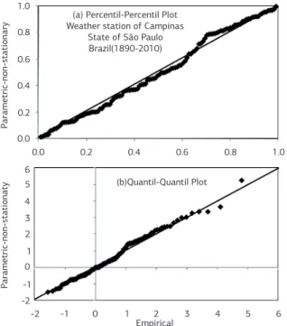
The small displacement of the Cartesian points in both PP and QQ plots (Figure 2) supports our decision in using model 3 to represent the probability density func-tion [Pr(Tminabst=1, Tminabst=2,…,Tminabst=n)].
In order to provide an example of the use of this non-stationary model, the probability associated with 5 ºC, 4 ºC, 3 ºC, 2 ºC and, 1 ºC at the years of 2020, 2030, 2040 and 2050 are presented in Table 2 (for more in-formation about the relationship between Tminabs values and frost occurrence see Sentelhas et al., 1995).
As can be seen, the probability of occurrence asso-ciated with the data presented in Table 2 tends in gen-eral to decrease over the years. This feature is a natural consequence of the increasing trends of the values of µt. However, within the analyzed period (2020-2050) mod-el 3 also indicates a continuous decrease in the rate of change of the probabilities of occurrence associated with the lowest Tminabs values (Table 2). Although this last feature seems contradictory with the increasing values of location parameter, it is worth emphasizing that model 3 also shows an increasing trend in the σ(t) values which indicates an increasing dispersion of the Tminabs values over the years. In other words, despite the fact that model 3 indicates an increasing trend in the average values of the Tminabs data, it does not give us enough evidence to adopt the speculation that extreme low temperatures (such as Tminabs < 2ºC) will no longer be observed at the weather station of Campinas. Also according to model 3 this trend will be accompanied by a increasing in the vari-ance of future Tminabs data. From an agrometeorological point of view, this greater dispersion may be linked with future frost events.
Table 1. Likelihood ratio test (Λ*) applied to distinct sub-periods of the annual extreme minimum air temperature series of Campinas, State of São Paulo, Brazil
Time Span μ* σ* ξ* l(.) Λ*
1891-2010 4.85 2.32 -0.32 -268.805
15.18; p<0.01 1891-1950 4.29 1.7 -0.16 -121.265
1951-2010 5.29 2.6 -0.37 -139.95 1891-1930 3.76 1.53 -0.16 -76.672
22.50; p<0.01 1931-1970 4.94 2.02 -0.27 -85.356
1971-2010 5.99 2.4 -0.18 -95.528
*μ, σ, ξ are, respectively, the parameters of location, scale and, shape of the general extreme value distribution). The maximized log likelihood function [l(.)] is also shown.
Table 2. Future probabilities of occurrence associated with extreme values of minimum air temperature (Pr[Tminabs])in the region of Campinas, State of São Paulo, Brazil
Year Pr[Tminabs<x; x=5, 4, 3, 2, 1 ºC]*
5 ºC 4 ºC 3 ºC 2 ºC 1 ºC
2020 (t=130) 0.366 0.255 0.168 0.104 0.060 2030 (t=140) 0.344 0.242 0.162 0.102 0.061 2040 (t=150) 0.326 0.232 0.158 0.102 0.062 2050 (t=160) 0.311 0.224 0.155 0.102 0.064 *The probabilities were obtained by using a non-stationary model GEV(xt; μt, σt, ξt) [µt=3.095 + 0.0301t, σ t= exp(0.316 + 0.0053t), ξ t= -0.177]. The standard errors of each parameter are, respectively, 0.307, 0.005, 0.140, 0.002 and, 0.072.
interesting. In this view, the study carried out by Cannon (2010), that specifies the parameters of the GEV by us-ing a probabilistic extension of the multilayer perceptron neural network, can be seen as an important future alter-native to overcome the linear approach adopted in this study.
4. conclusIon
A non-stationary GEV model in which the parameters of location and scale are expressed as time-dependent func-tions is recommended to describe the probabilistic struc-ture of the annual extreme minimum air temperastruc-ture se-ries available from the weather station of Campinas, State of São Paulo, Brazil. In addition, since two of the three parameters of this probabilistic model are significantly conditioned on time, the presence of climate trends in the analyzed time series becomes evident.
Although this non-stationary model has indicated an average increase in the values of the analyzed data (rep-resented by the time variability of µ), it does not allow us to conclude that the region of Campinas is now free from frost occurrence. The increasing temporal trend in the scale parameter reveals an increasing trend in the dis-persions of the data sample. This greater dispersion may be linked with future values of this variable that still may cause the death of plant tissues.
Figure 2. Supporting the use of the non-stationary model GEV(xt;
μt, σt, ξt) [µt=3.095 + 0.0301t, σ t= exp(0.316 + 0.0053t), ξt= -0.177; t→year]. Percentil-Percentil (a) and Quantil-Quantil (b) plots applied to annual extreme minimum air temperature series.
P
arametric-non-stationary
(a) Percentil-Percentil Plot Weather station of Campinas
State of São Paulo Brazil(1890-2010)
(b)Quantil-Quantil Plot
P
arametric-non-stationaty
Empirical
1.0 0.8
0.6 0.4
0.2 0.0
0.0 0.2 0.4 0.6 0.8 1.0
6 5
4
3
2
1
0
-1 -2
-2 -1
0 1 2 3 4 5 6
reFerences
ANDERSON, O.D. Time series analysis and forecasting: The Box-Jenkins approach, London and Boston: Butterworths 1976.
ASTOLPHO, F.; CAMARGO, M.B.P.; BARDIN, L. Probabilidades mensais e anuais de ocorrência de temperaturas mínimas do ar adversas à agricultura na região de Campinas (SP), de 1891 a 2000. Bragantia, v.63, p.141-147, 2004.
BLAIN, G.C.; PICOLI, M.C.A.; LULU, J. Análise estatística das tendências de elevação nas séries anuais de temperatura mínima do ar no Estado de São Paulo. Bragantia, v.68, p.807-815, 2009.
BLAIN, G.C., LULU, J. Considerações estatísticas relativas a seis séries mensais de temperatura do ar da Secretaria de Agricultura e Abastecimento do Estado de São Paulo. Revista Brasileira de Meteorologia, v.26, p.29-40, 2011.
CAMARGO, M.B.P.; PEDRO JÚNIOR, M.J.; ALFONSI, R.R.; ORTOLANI, A.A.; BRUNINI, O. Probabilidades de ocorrência de temperaturas mínimas absolutas mensais e anual no Estado de São Paulo. Bragantia, v.52, p.161-168, 1993.
CANNON, A.J. A flexible nonlinear modeling framework for nonstationary generalized extreme value analysis in hydroclimatology. Hydrological Process, v.24, p.673-685, 2010.
COLES, S. An introduction to statistical modeling of extreme value. London: Springer 2001.
FELICI, M.; LUCARINI, V.; SPERANZA, A.; VITOLO, R. extreme value statistics of the total energy in an intermediate-complexity model of the midlatitude atmospheric jet. Part II: trend detection and assessment. Journal of the Atmospheric Science, v.64, p.2159-214-75, 2007.
FURIó, D.; MENEU, V. Analysis of extreme temperatures for four sites across Peninsular Spain. Theoretical Applied Climatology, v.104, p.83-99, 2011.
IPCC. Climate Change2001: Impacts, adaptation and vulnerability, contribution of working group 2 to the third assessment report of the intergovernmental panel on climate change. HOUGHTON, J.T. (Ed.). Cambridge: University Press, 2001.
IPCC. Climate Change 2007: The Physical Science Basis, Contribution of Working Group I to the Fourth Assessment Report of the Intergovernmental Panel on Climate Change. HOUGHTON, J.T. (Ed.). Cambridge: University Press, 2007.
KENDALL, M.A.; STUART, A. The advanced theory of statistics. 2.ed. Londres: Charles Griffin, 1967. v.2, 690p.
LEADBETTER, M.R.; LINDGREN, G.; ROOTZEN, H. Extremes and Related Properties of Random Sequences and Processes. New York: Springer, 1983. 336p.
MANN, H.B. Non-parametric tests against trend. Econometrica 13, MathSciNet, 1945. p.245-259.
MÉNDEZ, F.J.; MENÉNDEZ, M.; LUCEñO, A.; LOSADA, I.J. Analyzing Monthly Extreme Sea Levels with a Time-Dependent GEV Model. Journal of Atmospheric and Oceanic Technology, v.24, p.894–911, 2007.
NADARAJAH, S.CHOI, D. Maximum daily rainfall in South Korea. Journal of Earth System Science, v.116, p.311-320, 2007.
PUJOL, N.; NEPPEL, L., SABATIER, R. Regional tests for trend detection in maximum precipitation series in the French Mediterranean region. Hydrological Sciences Journal, v.52, p.952-973, 2007.
SANSIGOLO, C.A. Distribuições de extremos de precipitação diária, temperatura máxima e mínima e velocidade do vento em Piracicaba, SP (1917-2006). Revista Brasileira de Meteorologia, v.23, p.341-346, 2008.
SENTELHAS, P.C.; ORTOLANI, A.A.; PEZZOPANE, J.R.M. Estimativa da temperatura mínima de relva e da diferença de temperatura entre o abrigo e a relva em noites de geada. Bragantia, v.54, p.437-445, 1995.
WILKS, D.S. Statistical methods in the atmospheric sciences. 2.ed. San Diego: Academic Press, 2006. 629p.
ZHANG, X.; HARVEY, K.D.; HOGG, W.D.; YUZYK, T.R. Trends in Canadian streamflow. Water Resource Research, v.37, p.987–999, 2001.