ISSN: 1809-4430 (on-line)
_________________________
1 Engª Agrônoma, Mestre, Centro de Ecofisiologia e Biofísica, Instituto Agronômico (IAC), Campinas - SP, Fone: (19) 32415188, Ramal 428, [email protected]
2 Engª Ambiental e Sanitarista, Mestranda, Centro de Ecofisiologia e Biofísica, Instituto Agronômico (IAC), Campinas - SP, [email protected]
3 Engº Agrícola, Prof. Doutor, Centro de Ecofisiologia e Biofísica, Instituto Agronômico (IAC), Campinas - SP, [email protected]
4 Pesquisadora do Centro de Pesquisas Meteorológicas e Climáticas Aplicadas a Agricultura da Universidade de Campinas - CEPAGRI/UNICAMP - Campinas - SP,[email protected]
CLIMATE TRENDS IN THE MUNICIPALITY OF PELOTAS, STATE OF RIO GRANDE DO SUL, BRAZIL
Doi:http://dx.doi.org/10.1590/1809-4430-Eng.Agric.v35n4p 769-777/2015
IZABELE B. KRUEL1, MONICA C. MESCHIATTI2, GABRIEL C. BLAIN3, ANA M. H. DE ÁVILA4
ABSTRACT: Changes in the frequency of occurrence of extreme weather events have been pointed out as a likely impact of global warming. In this context, this study aimed to detect climate change in series of extreme minimum and maximum air temperature of Pelotas, State of Rio Grande do Sul, (1896 - 2011) and its influence on the probability of occurrence of these variables. We used the general extreme value distribution (GEV) in its stationary and non-stationary forms. In the latter case, GEV parameters are variable over time. On the basis of goodness-of-fit tests and of the maximum likelihood method, the GEV model in which the location parameter increases over time presents the best fit of the daily minimum air temperature series. Such result describes a significant increase in the mean values of this variable, which indicates a potential reduction in the frequency of frosts. The daily maximum air temperature series is also described by a non-stationary model, whose location parameter decreases over time, and the scale parameter related to sample variance rises between the beginning and end of the series. This result indicates a drop in the mean of daily maximum air temperature values and increased dispersion of the sample data.
KEYWORDS: general extreme value distribution, time dependent model, extreme weather events.
TENDÊNCIAS CLIMÁTICAS NO MUNICÍPIO DE PELOTAS, ESTADO DO RIO GRANDE DO SUL, BRASIL
RESUMO: Alterações na frequência de ocorrência dos eventos meteorológicos extremos têm sido apontadas como um provável impacto do aquecimento global. Nesse contexto, objetivou-se detectar a presença de alterações climáticas em séries de temperatura do ar mínima e máxima extrema s de Pelotas, Rio Grande do Sul (1896-2011), quantificando sua influência na probabilidade de ocorrência dessas variáveis. Utilizou-se da distribuição geral de valores extremos (GEV) empregada em suas formas estacionária e não estacionárias. Nesse último caso, os parâmetros da GEV são variáveis ao longo do tempo. Com base em testes de aderência e no método da razão da máxima verossimilhança, verificou-se que um modelo GEV em que o parâmetro de localização se eleva ao longo do tempo, apresenta o melhor ajuste da série de temperatura mínima diária. Esse resultado descreve significativa elevação na média dos valores dessa variável, indicando potencial redução na frequência do fenômeno geada. A série de temperatura máxima diária é também descrita por um modelo não estacionário, cujo parâmetro de localização decresce ao longo do tempo e o de escala, relacionado à variância amostral, eleva-se entre o início e o fim da série. Esse resultado indica queda na média dos valores de temperatura máxima diária e elevação da dispersão dos dados amostrais.
INTRODUCTION
Climate changes in the intensity and frequency of occurrence of extreme weather events have been identified as one of the most likely consequences of global warming (IPCC, 2007). Considering this hypothesis, authors like El Adlouni et al. (2007), Furió and Meneu (2011), Kayano and Sansigolo (2009), Sugahara et al. (2009) and Blain (2011a, b) have striven to detect climate trends in meteorological time series and to incorporate these changes in the estimation of their probability of occurrence (WILKS, 2011). In this way, Khaliq et al. (2009) argued that the use of parametric methods allow the identification of the presence of climate trends, and also enable to quantify the influence of this last component on the probability of occurrence of the variable under study.
Regarding the temporal variability of extreme weather events, studies such as IPCC (2007) indicate that the intensity and frequency of these events will change over time due to global warming. Collins et al (2009) also state that the maximum and minimum of global temperature has increased since the 1950. Similarly to the report of IPCC (2007), these authors observed that the increase in atmospheric CO2 is the main factor responsible for this increase. Alexander et al. (2006)
analyzed data from extreme atmospheric temperature on the daily scale and identified a significant increase in nighttime temperatures in 70% of evaluated regions.
On the basis of several indices associated with atmospheric temperature, Vincent et al. (2005) described the presence of significant upward trends in minimum temperature values in South America, and indicated the lack of consistent changes in the indices related to the maximum temperature. For the municipality of Santa Maria, State of Rio Grande do Sul (RS), Streck et al. (2011) demonstrated a significant increase in the minimum temperature of the grass, taken at 5 cm from the grassy ground, in the period from 1970 to 2009 for the months of April, June, October, November and December. With data of minimum temperature from various localities in the State of Rio Grande do Sul, Berlato and Althaus (2010) observed the lack of significant increase in the data across the state over the past 65 years. On the other hand, Sansigolo and Kayano (2010) examined six municipalities in RS and detected a significant warming in annual and seasonal series of minimum air temperature (Tmin), and a significant cooling for seasonal series (summer) of maximum air temperature (Tmax).
On the standpoint of detection and incorporation of climate trends in estimation of the probability of occurrence of extreme weather events, Co les (2001), Furió and Meneu (2011), Delgado et al. (2010), Blain (2011a, b), among others, described a way of using the general extreme value distribution (GEV) as a parametric method to detect and model trends in time series. In these studies, GEV parameters are estimated according to the covariate time, originating the non-stationary approach (NSGEV). The conclusion that the use of a NSGEV model leads to better probabilistic description of a sample in relation to that obtained by GEV model with constant parameters over time (stationary), it is a statistical indication of the presence of (climatic) trends in the studied series (DELGADO et al., 2010; BLAIN, 2011a, b, among others). Moreover, it is worth mentioning that air temperature affects virtually all human activities including agriculture. In this view, several studies have been carried out to evaluate the interactions between climate and food production (Furió and Meneu, 2011).
Given the above, the present study described the probabilistic structure of series of extreme minimum and maximum air temperatures from the weather station of Pelotas, State of Rio Grande do Sul, Brazil (1896-2011) on the basis of general extreme value distribution in its stationary and non-stationary forms.
MATERIAL AND METHODS
As described by Blain and Camargo (2012), the probability density function of GEV is described by:
t t t t t t tt M M
x f 1 1 1 1 exp 1 1 ) ( If
M 1> 0 (1)
GEV parameters were estimated by the maximum likelihood method, as recommended by Coles (2001). In order to incorporate the possible presence of climate trends in the estimation of the probability of occurrence of Tmin and Tmax, we proposed the following GEV models:
Model 1: GEV(µt=µ, σ t= σ, ξ t= ξ) – Stationary.
Model 2: GEV(µt= µo + βt, σ t= σ, ξ t= ξ) –homoscedastic model; β is the rate of change of the
location parameter.
Model 3: GEV(µt=µ’o + β’t, σ t= exp(σo + αt), ξ t= ξ) – The exponential function ensures that the
scale parameter (relative to the distribution dispersion) always present positive values. Model 4: GEV(µt=µ’’o + β’’t, σ’ t= exp(σ’o + α’t), ξ t= ξo + δt)
Model 1 is a particular case of model 2. By analogy, the models 1 and 2 are particular cases of model 3 which, in turn, is a particular case of model 4. The parameters of the models 1 to 4 were obtained by maximizing the likelihood function below, in which t = 1 refers to t = 1896 and t=116 refer to 2011:
116 1 1 1 1 1 * 1 exp 1 , , ; t t t t t t t t t t t t t t n t t x x x L
61 1 1 1 exp exp * exp 1 * t t t t t t t t t x x t (2) To check the adjustment of the observed data to the GEV, we initially used tests of Kolmogorov-Smirnov/Lilliefors (KSL) and Anderson-Darling (AD; ANDERSON and DARLING, 1952). As already described in other studies like Wilks (2011) and Teixeira et al. (2011), the KSL test is more suitable for assessing the central part of the distributions. In relation to the extreme values statistics, the AD test relies on the sum of squares of differences between theoretical and empirical distributions and on a weight function [Ψ(.)]), which gives greater emphasis, compared to KSL, to discrepancies in both ends (tails) of the respective curves (SHIN et al., 2012).Equation 3 describes the AD test.
N F . G. 2 .dG .
Qn
(3)
where,
N is the series length;
G(.) is the theoretical cumulative distribution; F(.) is the empirical distribution, and
The analysis of the equation 3 indicates that the AD test weights similarly the upper and lower tails of the distributions. It is noteworthy that the study of extreme values of Tmin is evidently directed to the lower tails of probability functions, while analysis of Tmax data is directed to the upper tail of the distributions. Thus it is necessary to use a Ψ(.) function capable of separately emphasize discrepancies in the upper and lower tails of the probability curves (SHIN et al., 2012). Ahmad et al. (1988) described an adaptation of AD test, in which Ψ (.) can be matched to [1-G(.)]-1 (equation 4), for emphasis on upper tails or to [G(.)]-1 (equation 5), for emphasis on the lower tails.
. .
. 1
.
. 2
dG G
G F N AU
(4)
. .
. .
. 2
dG G
G F N AL
(5) GEV models were also subjected to a new selection based on the Akaike information criterion (equations 6 and 7).
Model
21
Model
2k fori 1to4AIC i i (6)
Modelj i
AIC
Modeli
AIC minimum
(.)
(7)
In which k is the number of parameters of each model i, 2l(.) is the maximized log-likelihood function of each Model i. According to Burnham and Anderson (2004), models with Δ(.) ≤ 2 can be used to estimate the probability of occurrence of the values of the variable under study.
The last stage of evaluation, applied only to selected models by the three goodness-of-fit tests (KSL, AD and AL/AU) and by the Akaike information criterion, employed the likelihood ratio test (D test) as described in Coles (2001). According to El Adlouni et al. (2007), the D test (equation 8)
is based on the uncertainty principle that states that when there is no statistical difference between two models, the simplest one, i.e., the one with the fewest parameters, should be adopted. Numerous studies applied the likelihood ratio test to the non-stationary GEV (COLES, 2001; EL ADLOUNI et al., 2007 and BLAIN, 2011c, among others).
l Modelj l Modeli
D2 1 0 for j>i; Mi
Mj (8)The statistical significance of D test was estimated according to the chi-square distribution with degrees of freedom equal to the difference between the number of parameters of the models j and i. P-values less than or equal to 0.05 indicate that the modelj is more appropriate than the modeli
for the probabilistic description of the Tmin series (COLES, 2001; EL ADLOUNI et al., 2007;
among others). The adopted model after three rounds of selection underwent a visual inspection of adjustment proposed by Coles (2001) and Wilks (2011) based on Quantile-Quantile plots (QQ). According to Wilks (2011) QQ plots are qualitative methods of checking the adjustment of parametric distributions, because they enabled the comparison of the observed data (Tmax and Tmin in this case) to the estimated by parametric distribution. QQ plots were prepared as recommended by Coles (2001).
RESULTS AND DISCUSSION
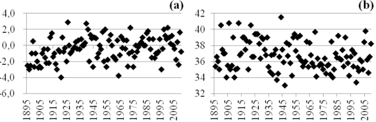
Figure 1 shows the values of Tmin and Tmax of Pelotas, State of Rio Grande do Sul, between 1896 and 2011.
FIGURE 1. Series of annual extreme temperatures available at the weather station of Pelotas, State of Rio Grande do Sul, Brazil (1896-2011) (a) Minimum temperature (b) Maximum temperature.
The results of the goodness-of-fit tests allowed us to infer that models 1 to 4 and models 3 and 4 can be used, respectively, to describe the probabilistic structure of the Tmin and Tmax (Table 1). In this respect, the Akaike information criterion indicated that only models 2 to 4 can be used to describe the probability of occurrence associated with Tmin and Tmax (Table 1).
TABLE 1. Results of the tests of Kolmogorov-Smirnov/Lilliefors (KSL), Anderson-Darling (AD), modified Anderson-Darling (AU/AL), respective critical values (crit) and Akaike Information Criterion Δ(.) for maximum (Tmax) and minimum (Tmin) temperature. Model KSL KSL crit AD AD crit AU AU crit Akaike Δ(.)
Tmax
1 0.06 0.07 0.73 0.59 0.47 0.28 1.28
2 0.07 0.07 0.65 0.60 0.44 0.28 1.66
3 0.06 0.07 0.54 0.59 0.34 0.34 0.00
4 0.06 0.07 0.49 0.68 0.31 0.38 0.35
Model KSL KSL crit AD AD crit AL AL crit Akaike Δ(.)
Tmin
1 0.04 0.07 0.34 0.64 0.21 0.29 7.59
2 0.05 0.07 0.20 0.64 0.11 0.30 0.00
3 0.05 0.07 0.19 0.64 0.12 0.29 1.89
4 0.05 0.08 0.23 0.73 0.15 0.32 0.50
With results obtained from the goodness-of-fit tests and according to the Akaike Information Criterion, we applied the likelihood ratio test (Table 2) to the models 2-3, 2-4 and 3-4 for Tmin and 3-4 for Tmax.
TABLE 2. Values related to the Likelihood Ratio Test for annual series of extreme values of minimum (Tmin) and maximum (Tmax) temperature of the city of Pelotas (1986-2011).
Models D Critical p-value
Tmin
2-3 0.112 3.842 0.74
2-4 3.503 5.992 0.17
3-4 3.391 3.842 0.06
As observed in Table 2 for Tmin data, there is no statistical difference between the three models. In this way, as recommended by Coles (2001) and El Adlouni et al. (2007), we adopted model 2 for the probabilistic description of the Tmin series. The parameters estimated were: μ t=-0.68130+0.01240t, σt=1.41554, ξt=-0.28120, with standard errors of: ±0.27146, ±0.00393, ±0.10166, ±0.05735, in this respective sequence. The model 2 describes an increase in the location parameter μ indicating a significant temporal increase in the mean value of Tmin. The mean rise in the Tmin values, described by model 2, also corroborates the assertion that frost events in the State of Rio Grande do Sul (1945-2005) were reduced by 3.5 days, on average, over the past ten decades (BERLATO; ALTHAUS, 2010). This last result is also consistent with IPCC (2007) that reports increasing trends in Tmin series observed in several regions of the Globe.
In relation to Tmax the statistics D (Table 2) selected the model 3, whose location and scale parameters are variable over time: μt=36.42-0.006t, σt=exp(0.68-0.004t), ξt=-0.13 with standard errors of: ±0.35, ±0.004, ±0.14 ±0.002 and ±0.08, in this respective sequence. In this context, the location parameter decreases over time indicating a temporal drop in mean values of Tmax. Nevertheless, this characteristic associated with μt is accompanied by an increase in the dispersion of Tmax values (high variance) described by temporal variation of the parameter σt. This result corroborates the study of Sansigolo and Kayano (2010), who detected a significant cooling trend of 0.6°C/100 years based on seasonal data (summer) from six localities of the State of Rio Grande do Sul, during the period from 1913 to 2006.
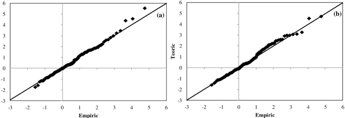
The visual inspection of Figure 2 confirms the results obtained by goodness-of-fit tests, Akaike information criterion and likelihood ratio test in the sense that the selected models are suitable to represent the probabilistic structure of Tmin and Tmax series. Moreover, the Cartesian points formed by values observed and estimated are, in general, close to the 1:1 line. In agreement with Coles (2001) and Wilks (2011), this characteristic indicates that adopted models can be used to estimate the probability of occurrence of the variable under study. Figure 2a (Tmin) presents a deviation from linearity only for the three highest values of this variable, suggesting a satisfactory fit to the lower extremes of Tmin.
At once, the visual comparison of Figures 2a and 2b suggests a slightly lower performance of the NSGEV model to describe the values of Tmax than those obtained for the description of Tmin.
FIGURE 2. Quantile-quantile plots resulting from adjusting series of daily minimum (a) and maximum (b) values of air temperature within each year to the general extreme value distribution for Pelotas, State of Rio Grande do Sul, Brazil (1896-2011).
As previously described After adopting a NSGEV model for the probabilistic description of air temperature data from four Spanish localities, Furió and Meneu (2011) estimated for the years 2020, 2050 and 2075, values of these atmospheric variables associated with different levels of probability. In the present study, in order to exemplify a possible practical application of the
-3 -2 -1 0 1 2 3 4 5 6
-3 -2 -1 0 1 2 3 4 5 6
T
eo
ri
c
Empiric
(a)
-3 -2 -1 0 1 2 3 4 5 6
-3 -2 -1 0 1 2 3 4 5 6
T
eo
ri
c
Empiric
adopted models, we estimated the probability of occurrence associated with different values of Tmin and Tmax (Table 3) for the same years used by Furió and Meneu (2011).
TABLE 3. Future probabilities of occurrence associated with extreme values of minimum air temperature (Pr [Tmin]) and maximum air temperature (Pr [Tmax]), in Pelotas, State of Rio Grande do Sul, Brazil.
T(°C) Pr(x≤T) [%] T(°C) Pr(x>T) [%]
Tmin 2020 2050 2075 Tmax 2020 2050 2075
2 87.0 81.9 75.8 35 75.7 69.8 63.4
1 66.3 58.5 50.4 36 47.5 38.2 29.9
0 39.7 32.2 25.3 37 22.8 15 9.5
-1 17.4 12.6 8.7 38 8.4 4.2 1.9
-2 4.9 2.9 1.6 39 2.3 0.8 0.2
As can be seen in Table 3, the cumulative probability associated with extreme minimum values of Tmin decreases over time. In a practical aspect it is verified, for example, that the probability of occurrence of Tmin values equal to or lower than 0°C decreases between the years 2020 and 2075, from 39.7% to 25.3%. Furthermore, for the other extreme of the distribution, the results in Table 3 describe an increase in the cumulative probability of occurrence associated with the upper tails of Tmax. In other words, the adopted model indicates, for example, that the probability of a Tmax value higher than 37°C will decrease between the years 2020 and 2075, from approximately 22.8% to 9.5%.
CONCLUSIONS
The general extreme value distribution, in its non-stationary form, is recommended to describe the probabilistic structure of series of daily extreme minimum and maximum temperature in the location of Pelotas, State of Rio Grande do Sul, Brazil. This feature may represent a statistical indication of the presence of climate change in that region.
The probability of occurrence of the minimum temperature should be calculated by a function whose location parameter increases over time. This function describes significant increase in the mean values of temperature indicating a reduction in the frequency of frosts events. The probability of occurrence of the maximum temperature can be evaluated by a model with location and scale parameters increasing and decreasing, respectively, over time. This last characteristic indicates a downward trend in mean temperature values associated with increased sample dispersion.
ACKNOWLEDGEMENTS
Thanks CAPES for the scholarship and IAC for the opportunity to take the graduate course.
REFERENCES
AHMAD, M. I.; SINCLAIR, C. D.; SPURR, B. D. Assessment of flood frequency models using empirical distribution function. Water Resource Research, Denver, v. 24, n. 8, p. 1323–1328, 1988.
ALEXANDER, L.V.; ZHANG, X.; PETERSON, T.C.; CAESAR, J.; GLEASON, B.; TANK, A.M.G; HAYLOC.K, M.; COLLINS, D.; TREVIN, B.; RAHIMZADEH, F.; TAGIPOU, A.; RUPA KUMAR, K.; REVADEKAR, J.; GRIFFITHS, G.; VINCENT, L.; STEPHENSON, D.; BURN, J.; AGUILLAR, E.; TAYLOR, M.; NEW, M.; ZHAI, P.; RUSTICUCCI, M.; VASQUEZ-AGUIRRE, J.L. Global observed changes in daily climate extremes of temperature and precipitation. Journal of Geophysical Research: Atmosphere, Washington, v.111, n. D05 109, 2006. DOI:
ANDERSON, T. W.; DARLING D. A. Asymptotic theory of certain ‘‘goodness-of-fit’’ criteria based on stochastic processes. The Annals of Mathe matical Statistics, Beachwood, v. 23, n. 2, p. 193-212, 1952.
BERLATO, M.A; ALTHAUS, D. Tendência observada da temperatura mínima e do número de dias de geada do Estado do Rio Grande do Sul. Pesquisa Agropecuária Gaúcha, Porto Alegre, v.16, n.1, p.7-16, 2010.
BLAIN, G. C. Cento e vinte anos de totais extremos de precipitação pluvial máxima diária em Campinas, Estado de São Paulo: análises estatísticas. Bragantia, Campinas, v. 70, n. 3, p. 722-728, 2011a.
BLAIN, G. C. Aplicação do conceito do índice padronizado de precipitação à série decendial da diferença entre precipitação pluvial e evapotranspiração potencial. Bragantia, Campinas, v. 70, n. 1, p. 234-245, 2011b.
BLAIN, G.C. Incorporating climate trends in the stochastic modeling of extreme minimum air temperature series of Campinas, state of São Paulo, Brazil. Bragantia, Campinas, v.70, n. 4, p.234-245, 2011c.
BLAIN, G.C.; CAMARGO, M.B.P. Probabilistic structure of an annual extreme rainfall series of a coastal area of the State of São Paulo, Brazil. Engenharia Agrícola, Jaboticabal, v .32, n. 3, maio/jun., 2012.
BLAIN, G. C.; KAYANO, M. T.; CAMARGO, M. B. P. D.; LULU, J. Variabilidade amostral das séries mensais de precipitação pluvial em duas regiões do Brasil: Pelotas-RS e
Campinas-SP. Revista Brasileira de Meteorologia, São José dos Campos, v. 24, n. 1, p. 1-11, 2009. BURNHAM, K.P.; ANDERSON, D.R. Multimodel inference: understanding AIC and BIC in model selection. Sociological Methods Research, Beverly Hills, v. 33, p. 261-304, 2004. Disponível em: <http://smr.sagepub.com/content/33/2/261>. Acesso em: 12 jan. 2011. DOI: 10.1177/0049124104268644.
COLES, S. An introduction to statistical modeling of extreme value. London: Springer 2001. COLLINS, J.M.; CHAVES, R.R.; MARQUES, V.S. Temperature variability over South America.
Journal of Climate, Boston, v. 22, p. 5854-5859, 2009.
DELGADO, J. M.; APEL, H.; MERZ, B. Flood trends and variability in the Mekong river.
Hydrology and Earth System Sciences, Kathenburg-Lindau, v. 14, n. 1, p. 407-418, 2010. EL ADLOUNI, S.; OUARDA, T. B. M. J.; ZHANG, X.; ROY, R.; BOBÉE, B. Generalized maximum likelihood estimators for the nonstationary generalized extreme value model. Wate r Resources Research, Washington, v. 43, n. 3410, p. 1-13, 2007.
FURIÓ, D.; MENEU, V. Analysis of extreme temperatures for four sites across Peninsular Spain.
Theoretical Applie d Climatology, Wien, v. 104, n. 1-2, p. 83-99, 2011.
IPCC. Climate Change 2007: The Physical Science Basis. Contribution of Working Group I to the Fourth Assessment Report of the Intergovernmental Panel on Climate Change,
Cambridge: Cambridge University Press, 2007.
KAYANO, M. T.; SANSIGOLO, C. Interannual to decadal variations of precipitation and daily maximum and minimum temperatures in southern Brazil. Theoretical and Applied Climatology, Wien, v. 97, p. 81-90, 2009.
SANSIGOLO, C. A.; KAYANO, M. T. Trends of seasonal maximum and minimum temperatures and precipitation in Southern Brazil for the 1913–2006 period. Theoretical and Applied
Climatology, Wien, v. 101, n. 1-2, p. 209-216, 2010.
SHIN, H.; JUNG, Y.; JEONG, C. Assessment of modified Anderson–Darling test statistics for the generalized extreme value and generalized logistic distributions. Stochastic Environme ntal Research and Risk Assessment, Berlin, v.26, n. 1, p. 105-114, 2012.
STRECK, N. A.; GABRIEL, L. F.; HELDWEIN, A. B.; BURIOL, G. A.; DE PAULA, M. G.Temperatura mínima de relva em Santa Maria, RS: climatologia, variabilidade interanual e tendência histórica. Bragantia, Campinas, v. 70, n. 3, p. 696-706, 2011.
SUGAHARA, S.; DA ROCHA, R. P.; SILVEIRA, R. Non-stationary frequency analysis of extreme daily rainfall in Sao Paulo, Brazil. International Journal of Climatology, Chichester, v. 29, n. 9, p. 1339-1349, 2009.
TEIXEIRA, C.F.A.; DAMÉ, R.C.F.; ROSSKOFF, J.L.C. Intensity-duration-frequency ratios obtained from annual records and partial duration records in the locality of Pelotas - RS, Brazil.
Engenharia Agrícola, Jaboticabal, v. 31, n. 4, p. 687-694, 2011.
VINCENT, L.A.; PETERSON, T.C.; BARROS, V.R.; MARINO, M.B.; RUSTICUCCI, M.; CARRASCO, G.; RAMIREZ, E.; ALVES, L.M.; AMBRIZZI, T.; BERLATO, M.A.; GRIMM, A.M.; MARENGO, J.A.; MOLION. L.; MONCUNILL, D.F.; REBELLO, E.; ANUNCIAÇÃO, Y.M.T.; QUINTANA, J.; SANTOS, J.L.; BAEZ, J.; CORONEL, G.; GARCIA, J.; TREBEJO, I.; BIDEGAIN, M.; HAYLOCK, M.R.; KAROLY, D. Observed trends in indices of daily temperature extremes in South America 1960-2000. Journal of Climate, Boston, v.18, n. 23, p.5011-5023, 2005.
![TABLE 3. Future probabilities of occurrence associated with extreme values of minimum air temperature (Pr [Tmin]) and maximum air temperature (Pr [Tmax]), in Pelotas, State of Rio Grande do Sul, Brazil](https://thumb-eu.123doks.com/thumbv2/123dok_br/15933002.677446/7.893.88.810.174.327/future-probabilities-occurrence-associated-extreme-temperature-temperature-pelotas.webp)
