Printed version ISSN 0001-3765 / Online version ISSN 1678-2690 http://dx.doi.org/10.1590/0001-3765201620150103
www.scielo.br/aabc
Geostatistical Approach for Spatial Interpolation of Meteorological Data
DeryA Ozturk1
and FAtMAGul kIlIc2
1
Department of Geomatics Engineering, Ondokuz Mayis University, Kurupelit Campus, 55139, Samsun, Turkey
2
Department of Geomatics Engineering, Yildiz Technical University, Davutpasa Campus, 34220, Istanbul, Turkey
Manuscript received on February 2, 2015; accepted for publication on March 1, 2016
ABStrAct
Meteorological data are used in many studies, especially in planning, disaster management, water resources
management, hydrology, agriculture and environment. Analyzing changes in meteorological variables is
very important to understand a climate system and minimize the adverse effects of the climate changes.
One of the main issues in meteorological analysis is the interpolation of spatial data. In recent years, with
the developments in Geographical Information System (GIS) technology, the statistical methods have been
integrated with GIS and geostatistical methods have constituted a strong alternative to deterministic methods
in the interpolation and analysis of the spatial data. In this study; spatial distribution of precipitation and
temperature of the Aegean Region in Turkey for years 1975, 1980, 1985, 1990, 1995, 2000, 2005 and 2010
were obtained by the Ordinary Kriging method which is one of the geostatistical interpolation methods,
the changes realized in 5-year periods were determined and the results were statistically examined using
cell and multivariate statistics. The results of this study show that it is necessary to pay attention to climate
change in the precipitation regime of the Aegean Region. This study also demonstrates the usefulness of
the geostatistical approach in meteorological studies.
key words:
geostatistical interpolation, geographic information system, ordinary kriging, meteorological
data.
Correspondence to: Derya Ozturk E-mail: [email protected]
INtrODuctION
Measurement and evaluation of the spatially distributed meteorological data have become important in
connection with climate-change impact studies, determination of water budgets at different temporal and
spatial scales, as well as validation of atmospheric and hydrological models. Meteorological data are
usually available from a limited number of meteorological stations (Hofierka et al. 2002), mostly because
it is not economically and technically possible to obtain meteorological data throughout the entire surface.
For this reason, spatial interpolation of the meteorological variables obtained from the certain sample points
is performed in order to create a model for the entire surface.
Spatial interpolation is the procedure of estimating the value of unsampled points using existing
as deterministic and geostatistical (Burrough and McDonnell 1998, Matthews 2002). Deterministic
interpolation techniques calculate the values of unsampled points and create surfaces from measured points,
based on either the extent of similarity or the degree of smoothing (Matthews 2002). Deterministic methods
do not use probability theory (Waters 1997). Geostatistical interpolation techniques use the statistical
properties of the measured points, quantify the spatial autocorrelation among the measured points and
account for the spatial configuration of the sample points around the estimation location (Matthews 2002).
Kriging is a geostatistical technique for optimal spatial estimation (Waller and Gotway 2004). Kriging
provides a solution to the problem of estimation based on a continuous model of stochastic spatial variation
and takes the variogram model (Webster and Oliver 2007). Today, with the developments in computer and
Geographical Information System (GIS) technologies, the statistical methods have been integrated with
GIS and the geostatistical methods have constituted a strong alternative to deterministic methods in the
interpolation of the spatial data. In addition, statistical methods to analyze the interpolated layers have
allowed a better understanding of the changes occurred in the specific time period.
Climate change is one of the biggest threats for the entire globe (Kropp 2015). Climate changes affect
the natural balance of the earth and ecosystems and whole life is disrupted (National Academy of Sciences
2009) Climate change is most often measured by changes in primary climate variables, such as temperature
and precipitation. These variables are the main drivers of climate changes (Sheffield and Wood 2012). For
this reason, to understand and monitor the changes and their causes and effects accurately, changes should
be determined both spatially and quantitatively and the results should be evaluated in detail.
In this study it is aimed to investigate the spatial distribution of precipitation and temperature of the
Aegean Region in Turkey for years 1975, 1980, 1985, 1990, 1995, 2000, 2005 and 2010 by the Ordinary
Kriging method and statistically examine the results using cell statistics and multivariate statistics to
understand the changes. This study demonstrates the usefulness of the geostatistical approach for both
interpolation of meteorological data and analysis and comparison of the results.
MAterIAlS AND MetHODS
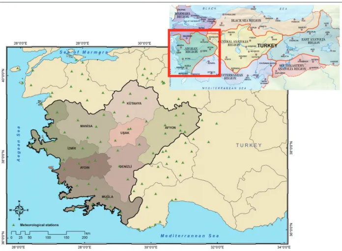
The Aegean Region is one of Turkey’s seven geographical regions. It is surrounded by the Aegean Sea
on the west and takes its name from the Aegean Sea (Ozcaglar 2014). In this study, the area comprising
eight provinces located in the Aegean Region has been analyzed. The total area is approximately 90,000
km
2(Figure 1). The coastal areas of the Aegean Region has a Mediterranean climate. The effects of the
Mediterranean climate extend up to 100-150 km inland from the coast. In coastal areas, winters are mild
and summers are very hot and dry. The interior side of the region is affected by the continental climate
(Sensoy et al. 2008).
CREATING AN ESTIMATION SURFACE lAYER WITH THE ORDINARY KRIGING
Estimation with the Kriging interpolation method has a two-step process:
(i) fitting a model:
creation of the
variograms and covariance functions to estimate the statistical dependence (spatial autocorrelation) values
that depend on the model of autocorrelation and
(ii)
making an estimation:
estimation of the unknown
values (ESRI 2014a).
The first step in the Ordinary Kriging is to create a semivariogram from the scatter point set to be
interpolated. A semivariogram consists of
(i) an empirical semivariogram
(experimental variogram) and
(ii) a model semivariogram
(GMS User Manuel 2012). Semivariogram is a mathematical model of the
semivariance as a function of
lag
and displays the statistical correlation of nearby points (Prasad et al.
2007). Spatial autocorrelation (means feature similarity) is based on both feature locations and feature
values simultaneously (not only based on feature locations or attribute values alone). Given a set of features
and an associated attribute, it evaluates whether the pattern expressed is clustered, dispersed, or random
(Matthews 2002). Empirical semivariogram, computed by (Eq.1) for all pairs of locations separated by
distance h (ESRI 2014a):
Semivariogram (distance h) = 0.5 * average[(value at location i – value at location j)
2] (1)
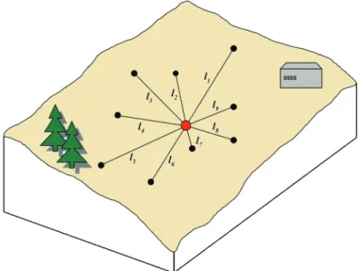
The formula involves calculating the difference squared between the values of the paired locations.
Figure 2 shows the pairing of one point (the red point) with all other measured locations. This process
continues for each measured point (ESRI 2014a).
Often, each pair of locations has a unique distance, and there are often many pairs of points. To plot all
pairs quickly becomes unmanageable. Instead of plotting each pair, the pairs are grouped into
lag bins
. The
empirical semivariogram is a graph of the averaged semivariogram values on the y-axis and the distance (or
lag
) on the x-axis (Figure 3) (ESRI 2014a).
When two locations are close to each other (far left on the x-axis of the semivariogram cloud), then
they are expected to be similar (low on the y-axis of the semivariogram cloud) (ESRI 2014a, Prasad et al.
2007).
“As pairs of locations become farther apart (moving to the right on the x-axis of the semivariogram
cloud), they should become more dissimilar and have a higher squared difference (moving up on the y-axis
of the semivariogram cloud)”
(ESRI 2014a).
Once the empirical variogram is obtained, the next step is to define a model semivariogram (GMS User
Manuel 2012). Semivariogram modeling is a main step between spatial description and spatial estimation.
The empirical semivariogram provides information on the spatial autocorrelation of datasets, however
does not supply information for all possible directions and distances. For this reason, it is necessary to fit
Figure 2 - Calculation of the difference squared between the paired locations.
a model (a continuous function or curve) to the empirical semivariogram (ESRI 2014a). There are many
semivariogram models. Some of the most common are linear, circular, spherical, exponential, and Gaussian
model (Li and Heap 2008). The selected model influences the estimation of the unknown values and each
model is designed to fit different types of phenomena more accurately (ESRI 2014a).
Once the model variogram is obtained, it is used to calculate the weights used in Kriging (GMS User
Manuel 2012). The basic equation used in the Ordinary Kriging is as (Eq.2) (ESRI 2014a, GMS User
Manuel 2012, Borga and Vizzaccaro 1996):
∑
= ∧
=
Ni
i i
Z
s
s
Z
1
0
)
(
)
(
λ
(2)
Where;
)
(
s
iZ
: the measured value at the
i
th location
i
λ
: an unknown weight for the measured value at the
i
th location
)
(
s
0: the estimation location
N: the number of measured values
With Kriging method, the value
Z
(
s
0)
∧
at the point
s
0, where the true unknown value is
Z
(
s
0)
, is estimated
by a linear combination of the values at N surrounding data points (Borga and Vizzaccaro 1996).
In the Ordinary Kriging, the weight,
λ
i, depends on a fitted model to the measured points, the distance to
the estimation point, and the spatial relationships among the measured values around the estimation location
(ESRI 2014a) and the Kriging weights are calculated by minimizing the variance (li and Heap 2008). The
Ordinary Kriging is the most widely used Kriging method (Wackernagel 2003) and this method assumes
that the data set has a stationary variance but also a non-stationary mean value within the search radius. The
Ordinary Kriging is highly reliable and recommended for most data sets (Vertical Mapper User Guide 2008).
StAtIStIcAl ANAlySeS OF lAyerS
CEll STATISTICS
In a local function, the value at each location on the output raster is a function of the input values at that
location. When computing a local function, input rasters can be combined and a statistic can be calculated.
In ArcGIS software, several cell statistics can be calculated for raster layers:
(i) MEAN:
Calculates the
mean (average) of the inputs,
(ii) MAXIMUM:
Determines the maximum (largest value) of the inputs,
(iii)
MEDIAN:
Calculates the median of the inputs,
(iv) MINIMUM:
Determines the minimum (smallest value)
of the inputs,
(v) RANGE:
Calculates the range (difference between largest and smallest value) of the inputs,
(vi) STD:
Calculates the standard deviation of the inputs (ESRI 2014b).
Multivariate Statistics
The multivariate statistics allow exploration of relationships between many different data layers or types of
reSultS AND DIScuSSION
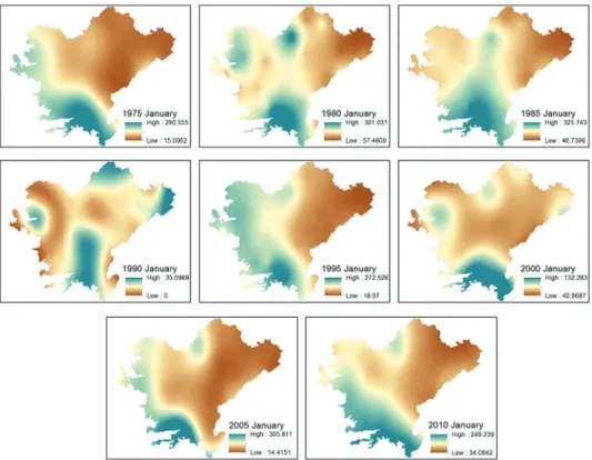
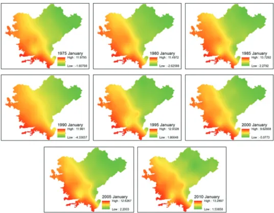
The time series of monthly precipitation and temperature data for the years 1975, 1980, 1985, 1990, 1995,
2000, 2005 and 2010 were used for preparing spatial distribution layers of precipitation and temperature
of the Aegean Region, Turkey. The Ordinary Kriging interpolation was applied for each month and a total
of 192 interpolations were performed (96 for precipitation and 96 for temperature) and grid layers with
250-meter pixel size were formed. The Ordinary Kriging interpolation results of the precipitation and
temperature data for January are shown in Figures 4 and 5, respectively.
Based on the multivariate statistics (band collection), spatial analyses were applied for the monthly
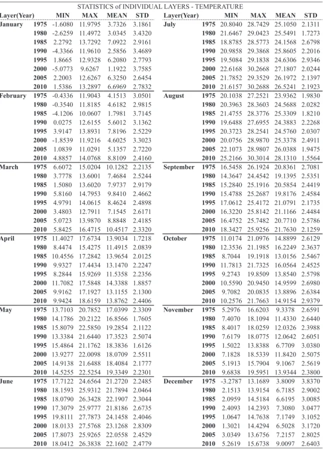
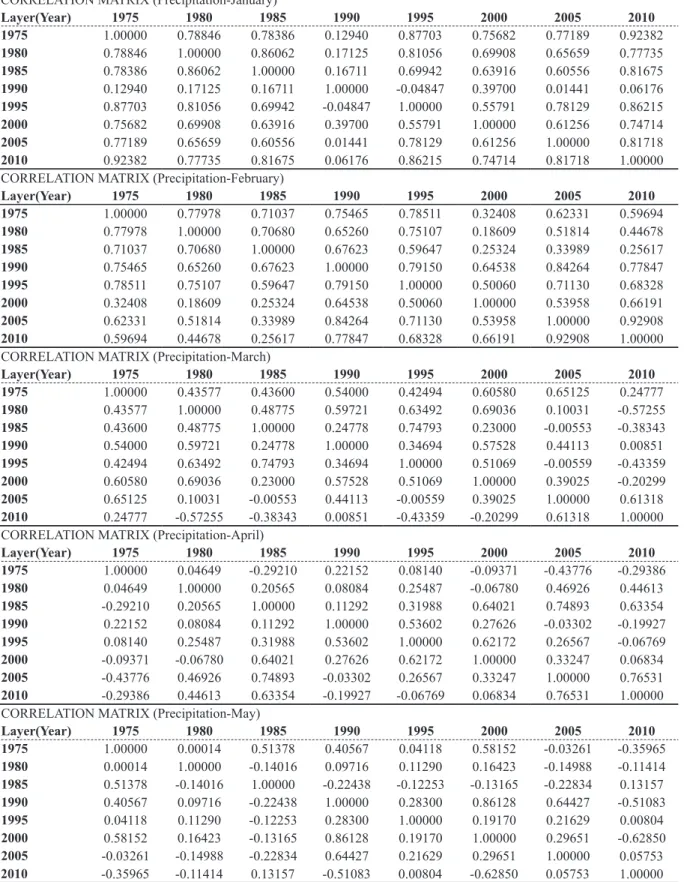
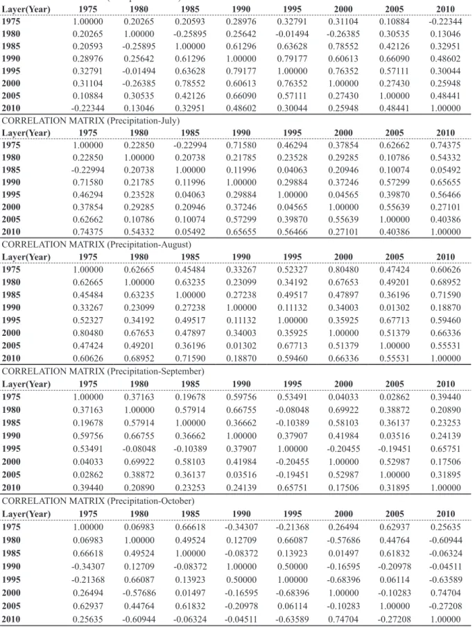
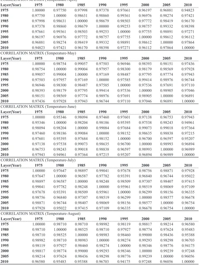
precipitation and temperature layer series which calculated by the Ordinary Kriging. Table I (for precipitation)
and Table II (for temperature) represent the main statistics, including the minimum, maximum, mean and
standard deviation values. In addition, the correlation coefficients were calculated with these analyses
(Tables III and IV).
When examining Table I, it was seen that the highest
“average precipitation”
and the highest
“precipitation”
values were in December 1990. Table II shows that both highest
“average temperature”
and highest
“temperature”
values were in August 2010.
According to Table III, correlation coefficients for precipitation are between -0.04847 and 0.92382
for January, 0.18609 and 0.92908 for February, -0.57255 and 0.74793 for March, -0.43776 and 0.76531
for April, -0.62850 and 0.86128 for May, -0.26385 and 0.79177 for June, -0.22994 and 0.74375 for July,
0.01302 and 0.80480 for August, -0.20455 and 0.69922 for September, -0.68396 and 0.74704 for October,
0.29150 and 0.85486 for November, 0.22520 and 0.90808 for December. According to Table IV, correlation
coefficients for temperature are between 0.95152 and 0.99524 for January, 0.95804 and 0.99591 for
February, 0.91016 and 0.99459 for March, 0.94823 and 0.99361 for April, 0.96744 and 0.99414 for May,
0.94961 and 0.99084 for June, 0.93391 and 0.99041 for July, 0.94175 and 0.99293 for August, 0.96714 and
0.99254 for September, 0.97214 and 0.99542 for October, 0.93409 and 0.99328 for November, 0.96537
and 0.99665 for December.
Correlations above 0.80 generally are accepted as high correlations. Correlations between 0.50 and
0.80 are usually considered as medium (moderate) correlations and correlations below 0.50 are typically
regarded as low correlations (Wang et al. 1990). Accordingly, very high correlation values were observed
between temperature values of years 1975, 1980, 1985, 1990, 1995, 2000, 2005 and 2010 for all months
(Table IV). But, the correlations between layers of precipitation were examined, both high and low
correlation values were observed. For precipitation layers, the highest correlation was observed between
the year of 1975 and 2010 for January; 2005 and 2010 for February; 1985 and 1995 for March; 2005 and
2010 for April; 1990 and 2000 for May; 1990 and 1995 for June; 1975 and 2010 for July; 1975 and 2000
for August; 1980 and 2000 for September; 2000 and 2010 for October; 2005 and 2010 for November; 1980
and 1990 for December.
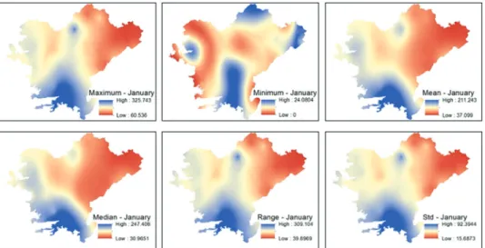
By calculating cell statistics, a statistic for each cell in an output raster can be calculated based on the
values of multiple input rasters (ESRI 2014b). In this study; maximum, minimum, mean, median, range
and standard deviation layers were produced by using precipitation and temperature layers for years 1975,
1980, 1985, 1990, 1995, 2000, 2005 and 2010 for all months. Totally 144 statistical layers were obtained
tABle I
Main statistics for precipitation layers (Minimum, Maximum, Mean, Standard deviation).
STATISTICS of INDIVIDUAl lAYERS - PRECIPITATION
layer(year) MIN MAX MeAN StD layer(year) MIN MAX MeAN StD
January 1975 15.0962 290.5551 105.2915 68.9066 July 1975 0.0000 11.4688 3.8647 3.2307
1980 57.4809 301.0310 144.8527 41.7206 1980 0.0000 6.4559 1.5206 0.9994
1985 46.7396 325.7432 160.8042 58.6881 1985 0.0000 7.6697 0.7246 0.7361
1990 0.0000 35.0969 12.1264 5.1998 1990 0.0000 39.4809 5.0383 5.5698
1995 18.9700 272.5263 120.9055 59.4265 1995 0.0000 189.5152 34.9476 30.6981
2000 42.8687 132.2835 69.6099 16.4874 2000 0.0000 23.2685 3.9946 4.4414
2005 14.4151 305.8113 70.4621 46.7614 2005 0.0000 85.0155 24.6473 19.6237
2010 34.0842 249.2391 114.5032 48.2253 2010 0.0173 12.8247 5.7179 3.1505
February 1975 35.9389 164.3231 58.1565 23.4616 August 1975 0.0000 66.0855 12.1734 13.2959
1980 11.4949 100.1111 35.0220 14.2885 1980 0.0000 29.5959 4.3619 5.3946
1985 29.6399 149.1992 73.9867 26.1003 1985 0.0000 41.5747 10.0517 7.4810
1990 7.0911 143.2509 49.7590 25.1979 1990 0.4801 67.0008 10.8518 7.5046
1995 6.6114 117.6134 27.3189 15.0847 1995 0.2385 16.9660 7.1374 3.8129
2000 49.3334 109.7159 86.5541 15.9437 2000 0.0000 26.2174 6.2557 5.7277
2005 18.2838 330.9904 117.0124 68.6871 2005 0.4208 17.9898 8.6525 4.3138
2010 47.3964 343.1137 151.4875 62.9992 2010 0.0000 20.6179 7.7861 5.9152
March 1975 26.2257 107.8506 64.0406 15.5155 September 1975 0.0000 49.7015 10.9055 10.0935
1980 49.5541 159.2850 95.6635 22.8128 1980 0.0000 55.4421 16.4988 14.7347
1985 27.8837 106.6610 59.4646 17.9716 1985 0.0000 6.5261 1.9362 1.3202
1990 6.9016 39.8629 23.6062 5.8286 1990 1.4236 38.1317 20.5715 8.0680
1995 61.6728 222.2994 126.3867 33.2200 1995 0.0000 46.1658 17.5078 11.7651
2000 38.4527 143.0037 88.8729 20.7716 2000 0.0000 22.9868 5.9550 5.8907
2005 33.6981 117.8575 79.2205 15.7518 2005 4.7207 35.6864 15.2393 6.0027
2010 2.0541 66.2231 30.9691 13.4006 2010 22.0556 44.4905 33.0731 4.0500
April 1975 18.2819 98.7922 51.6425 12.2515 October 1975 9.5328 90.6642 33.0401 13.0100
1980 29.4372 69.5153 47.0104 7.3046 1980 4.3897 46.2036 22.3987 9.1381
1985 2.0838 44.1912 19.7078 9.1412 1985 11.1300 151.5788 42.3043 26.9946
1990 19.9863 90.5741 54.8812 12.3692 1990 7.2120 42.6564 24.6231 8.0837
1995 18.1657 89.0869 51.9969 14.4514 1995 6.0607 56.4756 34.5488 14.9560
2000 26.9695 152.4105 85.1713 26.0013 2000 3.6411 98.6216 34.3385 19.8806
2005 15.9945 90.1445 39.7732 13.9404 2005 11.2323 121.7506 33.1998 17.9017
2010 9.5546 83.4186 37.2400 14.8342 2010 49.5620 311.1042 116.5370 49.2287
May 1975 39.9216 119.2508 71.7452 17.9338 November 1975 39.6952 239.7979 112.4898 38.7931
1980 10.6646 77.5801 36.4267 10.0239 1980 31.0222 174.3634 93.1593 26.5030
1985 1.4462 92.5336 33.3793 9.2920 1985 28.2310 180.9006 85.0800 32.2572
1990 0.0000 62.5613 23.3644 13.0269 1990 13.8738 74.1966 32.1743 11.6332
1995 0.0000 76.9429 27.1503 9.6845 1995 31.6046 177.6392 88.1167 27.7271
2000 1.0087 79.3443 31.0651 20.8717 2000 1.8513 201.2959 54.5331 44.2754
2005 6.2719 83.2165 44.0559 17.0640 2005 43.2833 254.8676 114.4541 41.6780
2010 12.1662 46.3693 26.6590 6.6865 2010 8.2926 51.3080 28.8157 9.8915
June 1975 15.4860 100.2484 50.0390 17.3824 December 1975 39.7735 188.7916 88.9672 25.1946
1980 0.0000 80.8975 24.9794 12.4476 1980 28.2021 296.8829 147.5694 61.1975
1985 0.0000 45.2143 16.5010 11.0090 1985 19.9052 135.5423 51.3575 16.5321
1990 0.0000 54.2057 20.5578 14.1597 1990 43.9064 361.6299 165.4436 71.0610
1995 0.0021 47.5019 9.5297 10.6071 1995 24.6129 165.1980 71.9208 30.6091
2000 0.0000 37.4081 11.7682 8.3772 2000 14.4990 329.9915 52.2345 36.1115
2005 0.3222 58.3159 27.5195 12.8268 2005 11.9330 203.2546 65.3737 31.7432
tABle II
Main statistics for temperature layers (Minimum, Maximum, Mean, Standard deviation).
STATISTICS of INDIVIDUAl lAYERS - TEMPERATURE
layer(year) MIN MAX MeAN StD layer(year) MIN MAX MeAN StD
January 1975 -1.6080 11.9795 3.7326 3.1861 July 1975 20.8040 28.7429 25.1050 2.1311
1980 -2.6259 11.4972 3.0345 3.4320 1980 21.6467 29.0423 25.5491 1.7273
1985 2.2792 13.7292 7.0922 2.9161 1985 18.8785 28.5773 24.1568 2.6798
1990 -4.3366 11.9610 2.5856 3.4689 1990 20.9858 29.3868 25.8605 2.2016
1995 1.8665 12.9328 6.2080 2.7793 1995 19.5084 29.1838 24.6306 2.9346
2000 -5.0773 9.6267 1.1922 3.7585 2000 22.6168 30.2668 27.1807 2.0244
2005 2.2003 12.6267 6.3250 2.6454 2005 21.7852 29.3529 26.1972 2.1397
2010 1.5386 13.2897 6.6969 2.7832 2010 21.6157 30.2688 26.5241 2.1923
February 1975 -0.4336 11.9043 4.1513 3.0501 August 1975 20.1038 27.2521 23.9362 1.9830
1980 -0.3540 11.8185 4.6182 2.9815 1980 20.3963 28.3603 24.5688 2.0282
1985 -4.1206 10.0607 1.7981 3.7145 1985 21.4755 28.3776 25.3309 1.8210
1990 0.0275 12.6155 5.6012 3.1362 1990 19.6488 27.6955 24.3883 2.2268
1995 3.9147 13.8931 7.8196 2.5229 1995 20.3723 28.2541 24.5760 2.0307
2000 -1.8539 11.9216 4.6025 3.3023 2000 20.0756 28.9870 25.3378 2.4911
2005 1.0839 11.0291 5.1357 2.7220 2005 22.1073 28.9807 26.0388 1.9475
2010 4.8857 14.0768 8.8109 2.4160 2010 25.2166 30.3014 28.1310 1.5564
March 1975 6.6072 15.0204 10.1282 2.2135 September 1975 16.5458 26.1924 20.8361 2.7081
1980 3.7778 13.6001 7.4684 2.5244 1980 14.3647 24.4542 19.1395 2.5351
1985 1.5080 13.6020 7.9737 2.9179 1985 15.2840 25.1916 20.5854 2.4419
1990 5.8160 14.7953 9.8410 2.4662 1990 15.4788 25.2687 19.8176 2.4584
1995 4.9791 14.0615 8.4624 2.4898 1995 17.0612 25.4172 21.0791 2.1735
2000 3.4803 12.7911 7.1545 2.6171 2000 16.3220 25.8142 21.1166 2.4484
2005 5.0723 13.9870 8.8848 2.4185 2005 16.4752 25.7482 20.7710 2.5786
2010 5.8425 16.4715 10.4517 2.3320 2010 18.3427 25.9256 21.7630 2.1259
April 1975 11.4027 17.6734 13.9034 1.7218 October 1975 11.0174 21.0976 14.8899 2.6129
1980 8.4474 15.4275 11.4915 2.0839 1980 12.3536 21.1985 16.2249 2.3637
1985 10.4556 17.2842 13.9654 2.0125 1985 8.7044 19.1918 13.0156 2.5467
1990 9.9327 17.4434 13.1470 2.2247 1990 11.7813 21.7325 16.0564 2.4525
1995 8.2844 15.9269 11.5358 2.2356 1995 9.2743 19.8509 13.8540 2.5798
2000 11.7082 17.5848 14.3388 1.8857 2000 10.5590 20.9450 14.9599 2.6980
2005 9.9162 17.1927 13.1155 2.1300 2005 9.7082 20.0835 13.8896 2.6384
2010 9.9424 18.6159 13.8762 2.4406 2010 10.2576 21.7663 14.9154 2.9379
May 1975 13.7103 20.7852 17.0399 2.3309 November 1975 5.2976 16.6203 9.3378 2.6591
1980 14.1786 20.2122 16.8566 1.7605 1980 7.4070 18.1094 11.4330 2.6440
1985 15.8079 22.5850 19.2854 2.1122 1985 8.4017 18.0259 12.0326 2.3988
1990 13.3384 21.6440 17.3523 2.5074 1990 7.6179 18.0775 12.0642 2.6051
1995 15.4864 21.1762 18.3836 1.6126 1995 1.5022 13.8388 6.7709 3.0380
2000 13.9277 22.0098 18.0709 2.5511 2000 7.1828 18.5339 11.8420 2.5075
2005 14.9138 21.6488 18.4084 2.1777 2005 5.1913 15.7904 9.1067 2.5619
2010 14.5255 22.5254 19.3349 2.2301 2010 9.6838 19.5951 13.9344 2.3800
June 1975 17.7122 24.6564 21.2720 2.2485 December 1975 -3.2787 13.1689 3.8009 3.8370
1980 18.1593 25.9312 21.7894 2.0464 1980 2.1513 13.9154 6.7185 2.9002
1985 18.0790 26.3428 22.1907 2.3044 1985 2.0959 14.5184 6.6195 3.0085
1990 17.3079 25.9777 21.8186 2.6735 1990 2.4093 14.2393 7.3080 3.0477
1995 19.8111 27.7873 24.1458 2.4046 1995 1.0647 14.7638 7.1749 3.1052
2000 18.0133 27.5768 23.1268 2.8309 2000 1.3021 14.4294 6.5028 3.1720
2005 17.8073 25.9265 22.0558 2.4529 2005 3.0349 13.6756 7.2157 2.8025
tABle III
correlation matrix for precipitation layers.
CORRElATION MATRIX (Precipitation-January)
layer(year) 1975 1980 1985 1990 1995 2000 2005 2010
1975 1.00000 0.78846 0.78386 0.12940 0.87703 0.75682 0.77189 0.92382
1980 0.78846 1.00000 0.86062 0.17125 0.81056 0.69908 0.65659 0.77735
1985 0.78386 0.86062 1.00000 0.16711 0.69942 0.63916 0.60556 0.81675
1990 0.12940 0.17125 0.16711 1.00000 -0.04847 0.39700 0.01441 0.06176
1995 0.87703 0.81056 0.69942 -0.04847 1.00000 0.55791 0.78129 0.86215
2000 0.75682 0.69908 0.63916 0.39700 0.55791 1.00000 0.61256 0.74714
2005 0.77189 0.65659 0.60556 0.01441 0.78129 0.61256 1.00000 0.81718
2010 0.92382 0.77735 0.81675 0.06176 0.86215 0.74714 0.81718 1.00000 CORRElATION MATRIX (Precipitation-February)
layer(year) 1975 1980 1985 1990 1995 2000 2005 2010
1975 1.00000 0.77978 0.71037 0.75465 0.78511 0.32408 0.62331 0.59694
1980 0.77978 1.00000 0.70680 0.65260 0.75107 0.18609 0.51814 0.44678
1985 0.71037 0.70680 1.00000 0.67623 0.59647 0.25324 0.33989 0.25617
1990 0.75465 0.65260 0.67623 1.00000 0.79150 0.64538 0.84264 0.77847
1995 0.78511 0.75107 0.59647 0.79150 1.00000 0.50060 0.71130 0.68328
2000 0.32408 0.18609 0.25324 0.64538 0.50060 1.00000 0.53958 0.66191
2005 0.62331 0.51814 0.33989 0.84264 0.71130 0.53958 1.00000 0.92908
2010 0.59694 0.44678 0.25617 0.77847 0.68328 0.66191 0.92908 1.00000 CORRElATION MATRIX (Precipitation-March)
layer(year) 1975 1980 1985 1990 1995 2000 2005 2010
1975 1.00000 0.43577 0.43600 0.54000 0.42494 0.60580 0.65125 0.24777
1980 0.43577 1.00000 0.48775 0.59721 0.63492 0.69036 0.10031 -0.57255
1985 0.43600 0.48775 1.00000 0.24778 0.74793 0.23000 -0.00553 -0.38343
1990 0.54000 0.59721 0.24778 1.00000 0.34694 0.57528 0.44113 0.00851
1995 0.42494 0.63492 0.74793 0.34694 1.00000 0.51069 -0.00559 -0.43359
2000 0.60580 0.69036 0.23000 0.57528 0.51069 1.00000 0.39025 -0.20299
2005 0.65125 0.10031 -0.00553 0.44113 -0.00559 0.39025 1.00000 0.61318
2010 0.24777 -0.57255 -0.38343 0.00851 -0.43359 -0.20299 0.61318 1.00000 CORRElATION MATRIX (Precipitation-April)
layer(year) 1975 1980 1985 1990 1995 2000 2005 2010
1975 1.00000 0.04649 -0.29210 0.22152 0.08140 -0.09371 -0.43776 -0.29386
1980 0.04649 1.00000 0.20565 0.08084 0.25487 -0.06780 0.46926 0.44613
1985 -0.29210 0.20565 1.00000 0.11292 0.31988 0.64021 0.74893 0.63354
1990 0.22152 0.08084 0.11292 1.00000 0.53602 0.27626 -0.03302 -0.19927
1995 0.08140 0.25487 0.31988 0.53602 1.00000 0.62172 0.26567 -0.06769
2000 -0.09371 -0.06780 0.64021 0.27626 0.62172 1.00000 0.33247 0.06834
2005 -0.43776 0.46926 0.74893 -0.03302 0.26567 0.33247 1.00000 0.76531
2010 -0.29386 0.44613 0.63354 -0.19927 -0.06769 0.06834 0.76531 1.00000 CORRElATION MATRIX (Precipitation-May)
layer(year) 1975 1980 1985 1990 1995 2000 2005 2010
1975 1.00000 0.00014 0.51378 0.40567 0.04118 0.58152 -0.03261 -0.35965
1980 0.00014 1.00000 -0.14016 0.09716 0.11290 0.16423 -0.14988 -0.11414
1985 0.51378 -0.14016 1.00000 -0.22438 -0.12253 -0.13165 -0.22834 0.13157
1990 0.40567 0.09716 -0.22438 1.00000 0.28300 0.86128 0.64427 -0.51083
1995 0.04118 0.11290 -0.12253 0.28300 1.00000 0.19170 0.21629 0.00804
2000 0.58152 0.16423 -0.13165 0.86128 0.19170 1.00000 0.29651 -0.62850
2005 -0.03261 -0.14988 -0.22834 0.64427 0.21629 0.29651 1.00000 0.05753
tABle III (continuation)
CORRElATION MATRIX (Precipitation-June)
layer(year) 1975 1980 1985 1990 1995 2000 2005 2010
1975 1.00000 0.20265 0.20593 0.28976 0.32791 0.31104 0.10884 -0.22344
1980 0.20265 1.00000 -0.25895 0.25642 -0.01494 -0.26385 0.30535 0.13046
1985 0.20593 -0.25895 1.00000 0.61296 0.63628 0.78552 0.42126 0.32951
1990 0.28976 0.25642 0.61296 1.00000 0.79177 0.60613 0.66090 0.48602
1995 0.32791 -0.01494 0.63628 0.79177 1.00000 0.76352 0.57111 0.30044
2000 0.31104 -0.26385 0.78552 0.60613 0.76352 1.00000 0.27430 0.25948
2005 0.10884 0.30535 0.42126 0.66090 0.57111 0.27430 1.00000 0.48441
2010 -0.22344 0.13046 0.32951 0.48602 0.30044 0.25948 0.48441 1.00000 CORRElATION MATRIX (Precipitation-July)
layer(year) 1975 1980 1985 1990 1995 2000 2005 2010
1975 1.00000 0.22850 -0.22994 0.71580 0.46294 0.37854 0.62662 0.74375
1980 0.22850 1.00000 0.20738 0.21785 0.23528 0.29285 0.10786 0.54332
1985 -0.22994 0.20738 1.00000 0.11996 0.04063 0.20946 0.10074 0.05492
1990 0.71580 0.21785 0.11996 1.00000 0.29884 0.37246 0.57299 0.65655
1995 0.46294 0.23528 0.04063 0.29884 1.00000 0.04565 0.39870 0.56466
2000 0.37854 0.29285 0.20946 0.37246 0.04565 1.00000 0.55639 0.27101
2005 0.62662 0.10786 0.10074 0.57299 0.39870 0.55639 1.00000 0.40386
2010 0.74375 0.54332 0.05492 0.65655 0.56466 0.27101 0.40386 1.00000 CORRElATION MATRIX (Precipitation-August)
layer(year) 1975 1980 1985 1990 1995 2000 2005 2010
1975 1.00000 0.62665 0.45484 0.33267 0.52327 0.80480 0.47424 0.60626
1980 0.62665 1.00000 0.63235 0.23099 0.34192 0.67653 0.49201 0.68952
1985 0.45484 0.63235 1.00000 0.27238 0.49517 0.47897 0.36196 0.71590
1990 0.33267 0.23099 0.27238 1.00000 0.11132 0.34003 0.01302 0.18870
1995 0.52327 0.34192 0.49517 0.11132 1.00000 0.35925 0.67713 0.59460
2000 0.80480 0.67653 0.47897 0.34003 0.35925 1.00000 0.51379 0.66336
2005 0.47424 0.49201 0.36196 0.01302 0.67713 0.51379 1.00000 0.55531
2010 0.60626 0.68952 0.71590 0.18870 0.59460 0.66336 0.55531 1.00000 CORRElATION MATRIX (Precipitation-September)
layer(year) 1975 1980 1985 1990 1995 2000 2005 2010
1975 1.00000 0.37163 0.19678 0.59756 0.53491 0.04033 0.02862 0.39440
1980 0.37163 1.00000 0.57914 0.66755 -0.08048 0.69922 0.38872 0.20890
1985 0.19678 0.57914 1.00000 0.36662 -0.10389 0.58103 0.36137 0.23253
1990 0.59756 0.66755 0.36662 1.00000 0.37907 0.41984 0.03516 0.24139
1995 0.53491 -0.08048 -0.10389 0.37907 1.00000 -0.20455 -0.19451 0.65751
2000 0.04033 0.69922 0.58103 0.41984 -0.20455 1.00000 0.52987 0.17506
2005 0.02862 0.38872 0.36137 0.03516 -0.19451 0.52987 1.00000 0.31895
2010 0.39440 0.20890 0.23253 0.24139 0.65751 0.17506 0.31895 1.00000 CORRElATION MATRIX (Precipitation-October)
layer(year) 1975 1980 1985 1990 1995 2000 2005 2010
1975 1.00000 0.06983 0.66618 -0.34307 -0.21368 0.26494 0.62937 0.25635
1980 0.06983 1.00000 0.49524 0.12709 0.66087 -0.57686 0.44764 -0.60944
1985 0.66618 0.49524 1.00000 -0.08372 0.13923 0.01497 0.61832 -0.06324
1990 -0.34307 0.12709 -0.08372 1.00000 0.50000 -0.16595 -0.20978 -0.04511
1995 -0.21368 0.66087 0.13923 0.50000 1.00000 -0.68396 0.06114 -0.63589
2000 0.26494 -0.57686 0.01497 -0.16595 -0.68396 1.00000 -0.10283 0.74704
2005 0.62937 0.44764 0.61832 -0.20978 0.06114 -0.10283 1.00000 -0.27208
tABle III (continuation)
CORRElATION MATRIX (Precipitation-November)
layer(year) 1975 1980 1985 1990 1995 2000 2005 2010
1975 1.00000 0.79762 0.65602 0.45331 0.41620 0.62822 0.79794 0.72336
1980 0.79762 1.00000 0.77541 0.57684 0.59180 0.52085 0.72144 0.68886
1985 0.65602 0.77541 1.00000 0.63039 0.56208 0.64761 0.72962 0.73200
1990 0.45331 0.57684 0.63039 1.00000 0.34262 0.47725 0.34958 0.29150
1995 0.41620 0.59180 0.56208 0.34262 1.00000 0.45066 0.43236 0.34430
2000 0.62822 0.52085 0.64761 0.47725 0.45066 1.00000 0.64668 0.55346
2005 0.79794 0.72144 0.72962 0.34958 0.43236 0.64668 1.00000 0.85486
2010 0.72336 0.68886 0.73200 0.29150 0.34430 0.55346 0.85486 1.00000 CORRElATION MATRIX (Precipitation-December)
layer(year) 1975 1980 1985 1990 1995 2000 2005 2010
1975 1.00000 0.79379 0.25259 0.81574 0.78905 0.50197 0.86966 0.64845
1980 0.79379 1.00000 0.31704 0.90808 0.90569 0.39818 0.78649 0.80757
1985 0.25259 0.31704 1.00000 0.22520 0.48945 0.76838 0.31490 0.26742
1990 0.81574 0.90808 0.22520 1.00000 0.85097 0.42111 0.74077 0.78907
1995 0.78905 0.90569 0.48945 0.85097 1.00000 0.56697 0.77087 0.77156
2000 0.50197 0.39818 0.76838 0.42111 0.56697 1.00000 0.52801 0.38538
2005 0.86966 0.78649 0.31490 0.74077 0.77087 0.52801 1.00000 0.65563
2010 0.64845 0.80757 0.26742 0.78907 0.77156 0.38538 0.65563 1.00000
tABle IV
correlation matrix for temperature layers.
CORRElATION MATRIX (Temperature-January)
layer(year) 1975 1980 1985 1990 1995 2000 2005 2010
1975 1.00000 0.99001 0.98543 0.99064 0.98531 0.99384 0.99098 0.97266
1980 0.99001 1.00000 0.99524 0.98171 0.99200 0.99217 0.99463 0.97417
1985 0.98543 0.99524 1.00000 0.97166 0.99482 0.98869 0.99503 0.97539
1990 0.99064 0.98171 0.97166 1.00000 0.97136 0.98582 0.97629 0.95152
1995 0.98531 0.99200 0.99482 0.97136 1.00000 0.98977 0.99353 0.97975
2000 0.99384 0.99217 0.98869 0.98582 0.98977 1.00000 0.99041 0.97014
2005 0.99098 0.99463 0.99503 0.97629 0.99353 0.99041 1.00000 0.98280
2010 0.97266 0.97417 0.97539 0.95152 0.97975 0.97014 0.98280 1.00000 CORRElATION MATRIX (Temperature-February)
layer(year) 1975 1980 1985 1990 1995 2000 2005 2010
1975 1.00000 0.99420 0.99281 0.98748 0.98275 0.96240 0.98388 0.97305
1980 0.99420 1.00000 0.99591 0.99286 0.98342 0.97515 0.98280 0.96708
1985 0.99281 0.99591 1.00000 0.99162 0.98447 0.97700 0.98697 0.97381
1990 0.98748 0.99286 0.99162 1.00000 0.98965 0.98378 0.98806 0.97410
1995 0.98275 0.98342 0.98447 0.98965 1.00000 0.98594 0.98194 0.98254
2000 0.96240 0.97515 0.97700 0.98378 0.98594 1.00000 0.96256 0.95804
2005 0.98388 0.98280 0.98697 0.98806 0.98194 0.96256 1.00000 0.98685
2010 0.97305 0.96708 0.97381 0.97410 0.98254 0.95804 0.98685 1.00000 CORRElATION MATRIX (Temperature-March)
layer(year) 1975 1980 1985 1990 1995 2000 2005 2010
1975 1.00000 0.96776 0.93293 0.96541 0.98026 0.97802 0.96322 0.91016
1980 0.96776 1.00000 0.97682 0.97817 0.98798 0.98687 0.99252 0.96439
1985 0.93293 0.97682 1.00000 0.97683 0.95402 0.95607 0.96738 0.93709
1990 0.96541 0.97817 0.97683 1.00000 0.97132 0.97380 0.97428 0.93204
1995 0.98026 0.98798 0.95402 0.97132 1.00000 0.99459 0.98740 0.93968
2000 0.97802 0.98687 0.95607 0.97380 0.99459 1.00000 0.98191 0.93228
2005 0.96322 0.99252 0.96738 0.97428 0.98740 0.98191 1.00000 0.96909
tABle IV (continuation)
CORRElATION MATRIX (Temperature-April)
layer(year) 1975 1980 1985 1990 1995 2000 2005 2010
1975 1.00000 0.97750 0.97998 0.97378 0.97661 0.96197 0.96881 0.94823
1980 0.97750 1.00000 0.98631 0.98860 0.99361 0.96976 0.98274 0.97421
1985 0.97998 0.98631 1.00000 0.98679 0.98503 0.97772 0.98419 0.96170
1990 0.97378 0.98860 0.98679 1.00000 0.99253 0.98757 0.99332 0.98398
1995 0.97661 0.99361 0.98503 0.99253 1.00000 0.97755 0.98891 0.97271
2000 0.96197 0.96976 0.97772 0.98757 0.97755 1.00000 0.98612 0.96112
2005 0.96881 0.98274 0.98419 0.99332 0.98891 0.98612 1.00000 0.97864
2010 0.94823 0.97421 0.96170 0.98398 0.97271 0.96112 0.97864 1.00000 CORRElATION MATRIX (Temperature-May)
layer(year) 1975 1980 1985 1990 1995 2000 2005 2010
1975 1.00000 0.98754 0.99057 0.97503 0.96946 0.98393 0.98151 0.97436
1980 0.98754 1.00000 0.99004 0.97957 0.98300 0.98179 0.98569 0.97928
1985 0.99057 0.99004 1.00000 0.97169 0.98487 0.97795 0.97774 0.97943
1990 0.97503 0.97957 0.97169 1.00000 0.97585 0.99414 0.98976 0.96744
1995 0.96946 0.98300 0.98487 0.97585 1.00000 0.97536 0.97691 0.97110
2000 0.98393 0.98179 0.97795 0.99414 0.97536 1.00000 0.98905 0.97046
2005 0.98151 0.98569 0.97774 0.98976 0.97691 0.98905 1.00000 0.96891
2010 0.97436 0.97928 0.97943 0.96744 0.97110 0.97046 0.96891 1.00000 CORRElATION MATRIX (Temperature-June)
layer(year) 1975 1980 1985 1990 1995 2000 2005 2010
1975 1.00000 0.95346 0.98094 0.97460 0.97601 0.97138 0.96753 0.97943
1980 0.95346 1.00000 0.98204 0.98186 0.95395 0.97538 0.98243 0.94961
1985 0.98094 0.98204 1.00000 0.99084 0.97684 0.99073 0.99018 0.97364
1990 0.97460 0.98186 0.99084 1.00000 0.98152 0.98635 0.98838 0.97215
1995 0.97601 0.95395 0.97684 0.98152 1.00000 0.96700 0.96597 0.95207
2000 0.97138 0.97538 0.99073 0.98635 0.96700 1.00000 0.98993 0.96894
2005 0.96753 0.98243 0.99018 0.98838 0.96597 0.98993 1.00000 0.96989
2010 0.97943 0.94961 0.97364 0.97215 0.95207 0.96894 0.96989 1.00000 CORRElATION MATRIX (Temperature-July)
layer(year) 1975 1980 1985 1990 1995 2000 2005 2010
1975 1.00000 0.97647 0.98897 0.99041 0.97678 0.98756 0.98871 0.97928
1980 0.97647 1.00000 0.96587 0.97782 0.93391 0.96840 0.96744 0.95022
1985 0.98897 0.96587 1.00000 0.98248 0.98509 0.97307 0.98407 0.97415
1990 0.99041 0.97782 0.98248 1.00000 0.95961 0.98519 0.98069 0.97109
1995 0.97678 0.93391 0.98509 0.95961 1.00000 0.96299 0.98156 0.96335
2000 0.98756 0.96840 0.97307 0.98519 0.96299 1.00000 0.98577 0.96678
2005 0.98871 0.96744 0.98407 0.98069 0.98156 0.98577 1.00000 0.96754
2010 0.97928 0.95022 0.97415 0.97109 0.96335 0.96678 0.96754 1.00000 CORRElATION MATRIX (Temperature-August)
layer(year) 1975 1980 1985 1990 1995 2000 2005 2010
1975 1.00000 0.98710 0.98710 0.98982 0.98119 0.98817 0.98214 0.96580
1980 0.98710 1.00000 0.98525 0.98710 0.97927 0.98774 0.97624 0.95483
1985 0.98710 0.98525 1.00000 0.98983 0.98460 0.99000 0.98436 0.95388
1990 0.98982 0.98710 0.98983 1.00000 0.98274 0.99293 0.98298 0.96703
1995 0.98119 0.97927 0.98460 0.98274 1.00000 0.98346 0.98776 0.94175
2000 0.98817 0.98774 0.99000 0.99293 0.98346 1.00000 0.99239 0.97248
2005 0.98214 0.97624 0.98436 0.98298 0.98776 0.99239 1.00000 0.96056
(72 for precipitation and 72 for temperature). Figures 6 and 7 show the cell statistics of the precipitation and
temperature for the month of January.
Here, range layers give the most important information. Range layers indicate the difference between
the largest and the smallest value of the inputs. When examining the range layers, it was understood that the
month with largest changes is January for precipitation and November for temperature.
CORRElATION MATRIX (Temperature-September)
layer(year) 1975 1980 1985 1990 1995 2000 2005 2010
1975 1.00000 0.98432 0.98128 0.98609 0.97975 0.98318 0.98589 0.99125
1980 0.98432 1.00000 0.99155 0.98712 0.98378 0.98371 0.97888 0.97036
1985 0.98128 0.99155 1.00000 0.98127 0.97791 0.98163 0.97309 0.96714
1990 0.98609 0.98712 0.98127 1.00000 0.98041 0.97355 0.97007 0.98024
1995 0.97975 0.98378 0.97791 0.98041 1.00000 0.99027 0.98815 0.96733
2000 0.98318 0.98371 0.98163 0.97355 0.99027 1.00000 0.99254 0.97132
2005 0.98589 0.97888 0.97309 0.97007 0.98815 0.99254 1.00000 0.97438
2010 0.99125 0.97036 0.96714 0.98024 0.96733 0.97132 0.97438 1.00000 CORRElATION MATRIX (Temperature-October)
layer(year) 1975 1980 1985 1990 1995 2000 2005 2010
1975 1.00000 0.98886 0.99071 0.98472 0.99004 0.99062 0.99542 0.98544
1980 0.98886 1.00000 0.97972 0.98269 0.98005 0.98243 0.98307 0.97214
1985 0.99071 0.97972 1.00000 0.98881 0.99341 0.99234 0.98544 0.97534
1990 0.98472 0.98269 0.98881 1.00000 0.98608 0.98709 0.97632 0.97474
1995 0.99004 0.98005 0.99341 0.98608 1.00000 0.99196 0.98567 0.97342
2000 0.99062 0.98243 0.99234 0.98709 0.99196 1.00000 0.98698 0.98191
2005 0.99542 0.98307 0.98544 0.97632 0.98567 0.98698 1.00000 0.98408
2010 0.98544 0.97214 0.97534 0.97474 0.97342 0.98191 0.98408 1.00000 CORRElATION MATRIX (Temperature-November)
layer(year) 1975 1980 1985 1990 1995 2000 2005 2010
1975 1.00000 0.98838 0.99165 0.97041 0.98973 0.96630 0.99328 0.94459
1980 0.98838 1.00000 0.98876 0.98825 0.97959 0.97029 0.98830 0.96251
1985 0.99165 0.98876 1.00000 0.97865 0.98934 0.97822 0.98729 0.95602
1990 0.97041 0.98825 0.97865 1.00000 0.95958 0.97309 0.97731 0.97502
1995 0.98973 0.97959 0.98934 0.95958 1.00000 0.96471 0.98812 0.93409
2000 0.96630 0.97029 0.97822 0.97309 0.96471 1.00000 0.96795 0.96403
2005 0.99328 0.98830 0.98729 0.97731 0.98812 0.96795 1.00000 0.95475
2010 0.94459 0.96251 0.95602 0.97502 0.93409 0.96403 0.95475 1.00000 CORRElATION MATRIX (Temperature-December)
layer(year) 1975 1980 1985 1990 1995 2000 2005 2010
1975 1.00000 0.98203 0.98128 0.98008 0.98588 0.98097 0.96599 0.96537
1980 0.98203 1.00000 0.99205 0.99665 0.98918 0.99443 0.99171 0.97762
1985 0.98128 0.99205 1.00000 0.98926 0.98818 0.99459 0.98883 0.98108
1990 0.98008 0.99665 0.98926 1.00000 0.98819 0.99248 0.99313 0.98019
1995 0.98588 0.98918 0.98818 0.98819 1.00000 0.98769 0.98406 0.98327
2000 0.98097 0.99443 0.99459 0.99248 0.98769 1.00000 0.98867 0.97993
2005 0.96599 0.99171 0.98883 0.99313 0.98406 0.98867 1.00000 0.98158
2010 0.96537 0.97762 0.98108 0.98019 0.98327 0.97993 0.98158 1.00000
cONcluSIONS
Meteorological data are required in many fields such as environment, agriculture and management of natural
disasters where spatial data are used. But meteorological data are generally available from a limited number
of stations. For this reason, interpolation techniques are used to obtain complete surface information. In
recent years, depending on the technological developments in computer and GIS, geostatistical methods
are used in order to determine the spatial distribution of meteorological data and the Ordinary Kriging
method is nowadays a preferable option in the literature. Unlike the deterministic methods, geostatistical
interpolation techniques also utilize the statistical properties of the measured points. In geostatistical
techniques the autocorrelation among the measured points is determined and spatial configuration of the
sampling points around the estimation point is taken into consideration.
In this study, spatial distributions of precipitation and temperature of the Aegean Region in Turkey for
years 1975, 1980, 1985, 1990, 1995, 2000, 2005 and 2010 in 5-year periods were determined by the Ordinary
Figure 6 - Cell statistics of the precipitation for the month of January.
Kriging method. The time series of monthly precipitation and temperature data from 98 meteorological
stations were used for the Ordinary Kriging. To evaluate and interpret the results, multivariate statistics
(band collection) and cell statistics were applied for the monthly precipitation and temperature layer series.
The results revealed that a significant change in precipitation regime in the Aegean Region was occurred.
It is necessary to pay attention to this change because of multiple environmental effects of the climate
changes. In the following studies, prediction of the future trends and determination of the effects of these
changes on nature and human health are required.
reFereNceS
BORGA M AND VIzzACCARO A. 1996. On the interpolation of hydrologic variables: Formal equivalence of multiquadratic surface fitting and kriging. J Hydrol 195: 160-171.
BURROUGH PA AND MCDONNEll RA. 1998. Principles of Geographical Information Systems: Spatial Information Systems and Geostatistics. NewYork: Oxford University Press.
ESRI. 2014a. ArcGIS Resources - ArcGIS Help 10.2&10.2.1, http://resources.arcgis.com/en/help/main/10.2/ (accessed 03.03.2014). ESRI. 2014b. Statistical Analysis, http://www.esri.com/software/arcgis/extensions/spatialanalyst/key-features/statistical (accessed
12.02.2014).
GMS USER MANUAl. 2012. http://gmsdocs.aquaveo.com.s3.amazonaws.com/GMS_8.3_User_Manual.pdf (accessed 03.03.2014).
HOFIERKA J, PARAJKA J, MITASOVA H AND MITAS l. 2002. Multivariate interpolation of precipitation using regularized spline with tension. Trans GIS 6(2): 135-150.
KROPP S. 2015. Climate change and risk of flooding in Germany: Consequences for property values. In: Hepperle E, Dixon-Gough R, Mansberger R, Paulsson J, Reuter F and Yilmaz M (Eds), Challenges for Governance Structures in Urban and Regional Development. ETH zürich, p. 155-160.
lI J AND HEAP AD. 2008. A Review of Spatial Interpolation Methods for Environmental Scientists. Geoscience Australia Record 2008/23.
MATTHEWS SA. 2002. ArcGIS Geostatistical Analyst, GIS Resource Document 02-19. NATIONAl ACADEMY OF SCIENCES 2009. Ecological Impacts of Climate Change, USA.
OzCAGlAR A. 2014. Aegean Region, http://www.geography.humanity.ankara.edu.tr/ders_notu/cog_330.pdf (accessed 02.03.2014).
PRASAD R, DIXIT A, MAlHOTRA PK AND GUPTA VK. 2007. Geoinformatics in precision farming: An overview. In: Singh AK and Chopra UK (Eds), Geoinformatics Applications in Agriculture. New Delhi: New India Publishing Agency, p. 39-78. SENSOY S, DEMIRCAN M, UlUPINAR Y, BAlTA I. 2008. Climate of Turkey, http://www.mgm.gov.tr/files/en-us/
climateofturkey.pdf (accessed 02.03.2015).
SHEFFIElD J AND WOOD EF. 2012. Drought in the 21st Century. In: Drought: Past Problems and Future Scenarios. Routledge: Taylor & Francis, Chapter 8.
VERTICAl MAPPER USER GUIDE. 2008. http://reference.mapinfo.com/software/vertical_mapper/english/3_5/ VerticalMapperUserGuide.pdf (accessed 01.04.2015).
WACKERNAGEl H. 2003. Multivariate Geostatistics: An Introduction with Applications. Berlin : Springer-Verlag. WAllER lA AND GOTWAY CA. 2004. Applied Spatial Statistics for Public Health Data. New Jersey: J Wiley & Sons. WANG M, AIRHIHENBUWA CO AND NNADI-OKOlO E. 1990. Data analysis and selection of statistical methods. In:
Nnadi-Okolo E (Ed), Health Research Design and Methodology. Boca Raton: CRC Press, Chapter 4, p. 149-228.
WATERS NM. 1997. Spatial Interpolation, http://www.geog.ubc.ca/courses/klink/gis.notes/ncgia/u40.html#SEC40.3.3 (accessed 12.03.2014).