Délia Canha Gouveia Reis
DOCTORATE IN MATHEMATICSSPECIALTY: PROBABILITY AND STATISTICS
Extreme Rainfall in Madeira Island
DOCTORAL THESIS
Madeira Island
Thesis presented by
D´
elia Canha Gouveia Reis
and
unanimously approved on 12 December 2014
,
in public session to obtain the PhD Degree in Mathematics
Jury
Chairman:
Doctor Maria Teresa Alves Homem de Gouveia
(by delegation of authority of the Rector of the Universidade da Madeira)
Members of the Committee
(in alphabetical order)
:
Doctor Dinis Duarte Ferreira Pestana
Full Professor, Universidade de Lisboa
Doctor Jo˜
ao Alexandre Medina Corte-Real
Full Professor, Universidade de ´
Evora
Doctor Luiz Carlos Guerreiro Lopes
Assistant Professor, Universidade da Madeira
Doctor Rita Cabral Pereira de Castro Guimar˜
aes
Assistant Professor, Universidade de ´
Evora
Doctor Sandra Maria Freitas Mendon¸ca
Assistant Professor, Universidade da Madeira
Doctor S´ılvio Filipe Velosa
Abstract
Statistical Modelling of Extreme Rainfall in Madeira Island
Extreme rainfall events have triggered a significant number of flash floods in Madeira Island along its past and recent history. Madeira is a volcanic island where the spatial rainfall distribution is strongly affected by its rugged topography. In this thesis, annual maximum of daily rainfall data from 25 rain gauge stations located in Madeira Island were modelled by the generalised extreme value distribution. Also, the hypothesis of a Gumbel distribution was tested by two methods and the existence of a linear trend in both distributions parameters was analysed. Estimates for the 50– and 100–year return levels were also obtained. Still in an univariate context, the assumption that a distribution function belongs to the domain of attraction of an extreme value distribution for monthly maximum rainfall data was tested for the rainy season. The available data was then analysed in order to find the most suitable domain of attraction for the sampled distribution. In a different approach, a search for thresholds was also performed for daily rainfall values through a graphical analysis. In a multivariate context, a study was made on the dependence between extreme rainfall values from the considered stations based on Kendall’s
τ measure. This study suggests the influence of factors such as altitude, slope
orientation, distance between stations and their proximity of the sea on the spatial distribution of extreme rainfall. Groups of three pairwise associated stations were also obtained and an adjustment was made to a family of extreme value copulas involving the Marshall–Olkin family, whose parameters can be written as a function
of Kendall’s τ association measures of the obtained pairs.
Keywords: statistics of extremes, annual maxima method, extreme domain of attraction, threshold choice, copula functions, extreme rainfall.
Resumo
Modela¸c˜ao Estat´ıstica da Precipita¸c˜ao Extrema na Ilha da Madeira
Os extremos de precipita¸c˜ao constituem um factor importante na ocorrˆencia de cheias r´apidas como algumas que marcaram significativamente a hist´oria da Ilha da Madeira. Esta ilha de origem vulcˆanica apresenta diferentes regi˜oes relativamente aos extremos de precipita¸c˜ao condicionadas pela sua complexa orografia. Nesta tese, a fun¸c˜ao distribui¸c˜ao generalizada de valores extremos foi utilizada para modelar os m´aximos anuais dos valores di´arios de precipita¸c˜ao de 25 esta¸c˜oes situadas na Ilha da Madeira. Al´em disso, a hip´otese de escolha estat´ıstica da distribui¸c˜ao Gumbel foi testada por meio de dois m´etodos, tendo sido tamb´em analisada a existˆencia de tendˆencia linear nos parˆametros das duas distribui¸c˜oes. Foram tamb´em obtidas estimativas para n´ıveis de retorno de 50 e 100 anos. Ainda num contexto univariado, a suposi¸c˜ao de que a fun¸c˜ao de distribui¸c˜ao pertence ao dom´ınio de atra¸c˜ao de uma distribui¸c˜ao de valores extremos foi testada considerando os valores m´aximos
mensais de precipita¸c˜ao di´aria da ´epoca das chuvas. Foram depois aplicados
procedimentos para a escolha de dom´ınios de atra¸c˜ao para m´aximos considerando
os valores dispon´ıveis. Numa perspectiva distinta, foi tamb´em efectuada uma
procura de valores para o limiar de s´eries de valores di´arios de precipita¸c˜ao por meio de uma metodologia assente numa an´alise gr´afica. Num contexto multivariado, foi realizado um estudo sobre a dependˆencia entre extremos de precipita¸c˜ao na Ilha da Madeira assente na medida de associa¸c˜ao tau de Kendall, tendo sido formados grupos de trˆes esta¸c˜oes associadas duas a duas com os pares de esta¸c˜oes obtidos. Este estudo sugere a influˆencia da altitude, da orienta¸c˜ao das vertentes, da distˆancia entre esta¸c˜oes e da sua proximidade ao mar na distribui¸c˜ao espacial dos extremos de precipita¸c˜ao. Foi tamb´em realizado um ajuste a uma fam´ılia de c´opulas de extremos envolvendo a fam´ılia de Marshall–Olkin, cujos parˆametros podem ser escritos em fun¸c˜ao do tau de Kendall.
Palavras-chave: Estat´ıstica de extremos, modelo dos m´aximos anuais, dom´ınios de atra¸c˜ao, escolha do limiar, fun¸c˜oes c´opula, precipita¸c˜ao intensa.
Acknowledgements
To Professors Luiz Lopes and Sandra Mendon¸ca, my supervisors, for encouraging me to work in the area of extreme value analysis and for suggesting the topic of the present thesis. The generosity with which they offered their time and ideas to this work is also appreciated. I would also like to acknowledge their support and encouragement to participate in scientific meetings and their confidence in my work.
To the Portuguese Foundation for Science and Technology (FCT), for the financial support through the PhD grant SFRH/BD/39226/2007, financed by national funds of the Ministry of Science, Technology and Higher Education (MCTES). I am also grateful to the Centre of Statistics and Applications of the University of Lisbon (CEAUL) for the bibliographical and financial support through FCT projects PEst-OE/MAT/UI0006/2011 and PEst-OE/MAT/UI0006/2014. To the University of Madeira for providing the appropriate conditions for the realisation of this thesis and for the logistic support.
To the Portuguese Institute for Sea and Atmosphere (IPMA), namely to Doctor Victor Prior, for providing the monthly maximum rainfall data used in this thesis. Thanks are also due to the Department of Hydraulics and Energy Technologies of the Madeira Regional Laboratory of Civil Engineering (LREC), in particular to Doctor Carlos Magro, for making available the daily rainfall data from 25 rain gauge stations maintained in the past by the General Council of the Autonomous District of Funchal.
I would also like to express my gratitude and appreciation to all those I have had the opportunity and the pleasure to learn and work with directly in courses of Statistics and Probability: Professor Ana Abreu, Professor Paulo Freitas, Professor Rita Vasconcelos, Professor Sandra Mendon¸ca and Professor S´ılvio Velosa. A special acknowledgement to Professor Rita Vasconcelos for her guidance when I first needed to use a statistical software, for all the concise and fruitful meetings about the courses I taught as her assistant, and for all the encouragement throughout the elaboration of
this thesis. I would also like to thank Professors Rita Vasconcelos and Paulo Freitas for sparing me from the grading task in the last weeks of the second semester of the academic year 2013/2014, so that I could dedicate some more time to the conclusion of the writing of this thesis. I am also grateful to Professors Ana Abreu and S´ılvio Velosa for all their efforts to offer me precious time to dedicate to the elaboration of this thesis throughout the later five years. A special acknowledgement to Professor Ana Abreu for introducing me the R software and language, which was essential for the work developed and described here. I would also like to thank Professor Ana Abreu for the classes about the R software functionalities and also for the tips about R packages concerning maps, which were used in this thesis.
To all other colleagues at the Centre for Exact Sciences and Engineering for all their contributions to my education as a student and as a teacher. I am also grateful for their friendship and their support. A special acknowledgement to Professor Cust´odia Drumond for the encouragement, the care and also for the tea breaks which brightened many afternoons. A special acknowledgement to Professor Jos´e Carmo for having always assured me the best possible working conditions and for the constant encouragement throughout the elaboration of this thesis.
I would also like to express my appreciation to the participants of the scientific meetings organised by the Portuguese Society of Statistics (SPE) from whom I had the opportunity to learn. In particular, I would like to thank Professor Ivette Gomes for the encouraging comments and guidance about a work I presented in one of those meetings. A special acknowledgement to Professor Dinis Pestana for the guidance and bibliographical support.
To all my (present and former) students for the motivation that comes from the pleasure of lecturing to them.
To Maur´ıcio’s family (now also mine) for receiving me with open arms and also for their friendship, support and care.
To Analuce, my sister, for personifying the persistence in the pursuit of aims and
dreams. To L´ucia and Ant´onio, my parents, for personifying the strength and joy
of living. Thanks for all the support, care and love. I am blessed to have you three in my life.
Contents
List of Acronyms and Symbols xiii
List of Figures xv
List of Tables xxiii
1 Introduction 1
1.1 Aims and contributions . . . 2
1.2 Organization of the thesis . . . 5
2 State of the art (and a taste of the history of extreme value theory) 7 2.1 Univariate and multivariate extreme value approaches . . . 10
2.2 Application to rainfall extremes . . . 13
3 About Madeira Island’s climate characteristics, flash flood history and rainfall data 17 4 Methodology 29 4.1 Gumbel’s model approach . . . 29
4.1.1 Extreme value distributions . . . 30
4.1.2 Parameter estimation methods and statistical tests . . . 32
4.1.3 Plots and statistical tests for model diagnostics . . . 37
4.1.4 A trend analysis . . . 39
4.2 About extreme domains of attraction, number of observations above a random threshold and threshold choices . . . 41
4.3 An extreme value copula approach . . . 46
5 Results and discussion 57 5.1 Annual maxima – Gumbel’s model approach . . . 57
5.1.1 Dataset I . . . 58
5.1.2 Dataset II . . . 67
5.1.3 Dataset I+II . . . 81
5.2 Monthly and daily precipitation data – PORT and POT approaches . 89 5.2.1 Statistical choice of extreme domains of attraction . . . 90
5.2.2 Threshold choice in a POT approach . . . 97
5.3 Spatial annual maxima – Copula functions . . . 104
5.3.1 Dataset V . . . 106
5.3.2 Dataset VI . . . 112
5.3.3 Dataset VII . . . 121
6 Conclusion 129
References 137
Appendix
157
List of Acronyms and Symbols
ASI Advanced Statistical Institute
EVC extreme value copula
GEV generalised extreme value
GPD generalised Pareto distribution
IPMA Portuguese Institute for the Sea and Atmosphere
LREC Regional Laboratory of Civil Engineering
ML maximum likelihood
POT peaks over threshold
PORT peaks over random threshold
PWM probability weighted moments
d
−
→ converges in distribution to
dX,Y distance in meters between stations X and Y
b
qp 1/p–year return level estimate
b
qM
α 1/α–year return level estimate calculated by the method M (α∈(0,1))
χ2
k chi–square distribution withk degrees of freedom
rα return period of Eα =P(Xi > xi,α) for i∈ {1,2,3}and α∈(0,1)
Xi observation at the i–th rain gauge station
xi,q (1−q)–quantile of Xi for q∈(0,1) andi∈ {1,2,3}
x1:n, ..., xn:n ascending order statistics of the sample (x1, . . . , xn)
x(1), ..., x(k) exceedances
τX,Y
n estimates based on a sample of size n of Kendall’s τ association
measure between stationsX and Y
List of Figures
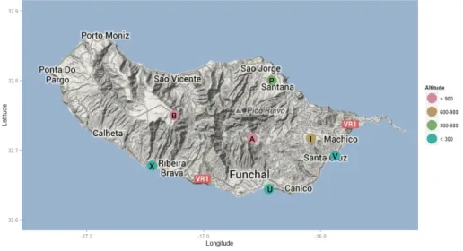
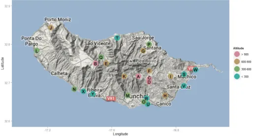
3.1 Location and altitude range of the rain gauge stations–Set LREC
(Map data c2014 Google). . . 20
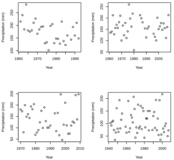
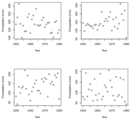
3.2 Annual maximum of daily precipitation values at Areeiro (A) (up
left), Bica da Cana (B) (up right), Santo da Serra (I) (down left), and Santana (P) (down right) stations–Set IPMA. . . 25
3.3 Annual maximum of daily precipitation values at Funchal (U) (up
left), Santa Catarina (V) (up right), and Lugar de Baixo (X) (down) stations–Set IPMA. . . 26
3.4 Annual maximum of daily precipitation values at Poiso (C) (up left),
Montado do Pereiro (D) (up right), Encumeada (E) (down left), and Ribeiro Frio (F) (down right) stations–Set LREC. . . 26
3.5 Annual maximum of daily precipitation values at Queimadas (G)
(up left), Camacha (H) (up right), and Porto Moniz (J) (down) stations–Set LREC. . . 27
3.6 Annual maximum of daily precipitation values at Curral das
Freiras (K) (up left), Ponta do Pargo (L) (up right), Santo Ant´onio (M) (down left), and Canhas (N) (down right) stations– Set LREC. . . 27
3.7 Annual maximum of daily precipitation values at Sanat´orio (O)
(up left), Loural (Q) (up right), and Bom Sucesso (R) (down) stations–Set LREC. . . 28
3.8 Annual maximum of daily precipitation values at Machico (S)
(up left), Ponta Delgada (T) (up right), Cani¸cal (W) (down left), and Ribeira Brava (Y) (down right) stations–Set LREC. . . 28
5.1 Location and altitude range of the rain gauge stations–Dataset I (Map
data c2014 Google). . . 58
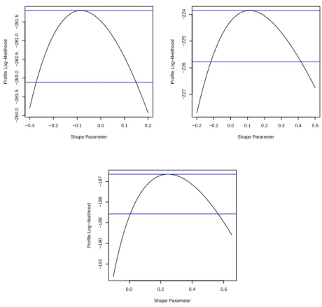
5.2 Profile log-likelihood for γ in Model 1 for Areeiro (A) (up left), Bica da Cana (B) (up right), Santo da Serra (I) (down left), and Santana (P) (down right) stations. . . 61
5.3 Profile log-likelihood forγ in Model 1 for Funchal (U) (up left), Santa
Catarina (V) (up right) and Lugar de Baixo (X) (down) stations. . . 62
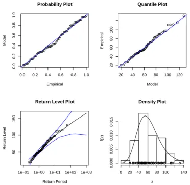
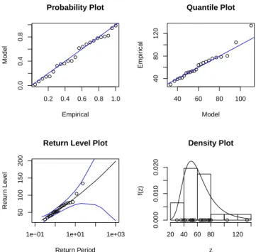
5.4 Diagnostic plots for non-Gumbel GEV fit to the Funchal (U) station
data–Dataset I. . . 65
5.5 Diagnostic plots for Gumbel fit to the Funchal (U) station data–
Dataset I. . . 65
5.6 Location and altitude range of the rain gauge stations–Dataset II
(Map data c2014 Google). . . 68
5.7 Annual maximum of daily precipitation values at Areeiro (A) (up
left), Bica da Cana (B) (up right), Santo da Serra (I) (down left), and Santana (P) (down right) stations–Dataset II. . . 71
5.8 Annual maximum of daily precipitation values at Funchal (U) (up
left), Santa Catarina (V) (up right), and Lugar de Baixo (X) (down) stations–Dataset II. . . 72
5.9 Diagnostic plots for GEV fit to the Ribeira Brava (Y) station data–
Dataset II. . . 78 5.10 Diagnostic plots for GEV fit to the Ponta Delgada (T) station data–
Dataset II. . . 78 5.11 Annual maximum daily precipitation values at Areeiro (A) (up left),
Bica da Cana (B) (up right), Santo da Serra (I) (down left), and Lugar de Baixo (X) (down right) stations–Dataset I+II. . . 83 5.12 Diagnostic plots for GEV distribution fit to the Santo da Serra (I)
station data–Dataset I+II. . . 87 5.13 Diagnostic plots for GEV ditribution fit to the Santa Catarina (V)
station data–Dataset I+II. . . 87 5.14 Location and altitude range of the rain gauge stations–Dataset III
(Map data c2014 Google). . . 90
5.15 Values of the test statisticEn(k) (solid) and the 0.95 quantile (dotted)
applied to the datasets from Areeiro (A) (up left), Santo da Serra (I) (up right) and Santana (P) (down) stations. . . 92 5.16 Values of the test statisticEn(k) (solid) and the 0.95 quantile (dotted)
5.17 Values of the test statisticsW∗
n (solid) andR∗n(dotted) applied to the
datasets from Areeiro (A) (up left), Bica da Cana (B) (up right) and
Santo da Serra (I) (down) stations. . . 95
5.18 Values of the test statisticsW∗ n (solid) andR∗n(dotted) applied to the datasets from Santana (P) (up left), Funchal (U) (up right), Santa Catarina (V) (down left) and Lugar de Baixo (X) (down right) stations. 96 5.19 Location and altitude range of the rain gauge stations–Dataset IV (Map data c2014 Google). . . 97
5.20 Mean residual plot for the Areeiro (A) (up left), Encumeada (E) (up right), Canhas (N) (down left) and Funchal (U) (down right) stations data. . . 98
5.21 Parameter stability plots for the Areeiro (A) station data. . . 99
5.22 Parameter stability plots for the Encumeada (E) station data. . . 99
5.23 Parameter stability plots for the Canhas (N) station data. . . 100
5.24 Parameter stability plots for the Funchal (U) station data. . . 100
5.25 Location and altitude range of the rain gauge stations–Dataset V (Map data c2014 Google). . . 106
5.26 Location and altitude range of the rain gauge stations–Dataset VI (Map data c2014 Google). . . 112
5.27 Location and altitude range of the rain gauge stations–Dataset VI (Map data c2014 Google). . . 122
A.1 Diagnostic plots for Gumbel fit to the Areeiro (A) station data– Dataset I. . . 160
A.2 Diagnostic plots for GEV fit to the Areeiro (A) station data–Dataset I.160 A.3 Diagnostic plots for Gumbel fit to the Bica da Cana (B) station data– Dataset I. . . 161
A.4 Diagnostic plots for GEV fit to the Bica da Cana (B) station data– Dataset I. . . 161
A.5 Diagnostic plots for Gumbel fit to the Santo da Serra (I) station data–Dataset I. . . 162
A.6 Diagnostic plots for GEV fit to the Santo da Serra (I) station data– Dataset I. . . 162
A.7 Diagnostic plots for Gumbel fit to the Santana (P) station data– Dataset I. . . 163
A.9 Diagnostic plots for Gumbel fit to the Santa Catarina (V) station data–Dataset I. . . 164 A.10 Diagnostic plots for GEV fit to the Santa Catarina (V) station data–
Dataset I. . . 164 A.11 Diagnostic plots for Gumbel fit to the Lugar de Baixo (X) station
data–Dataset I. . . 165 A.12 Diagnostic plots for GEV fit to the Lugar de Baixo (X) station data–
Dataset I. . . 165
C.1 Diagnostic plots for Gumbel fit to the Areeiro (A) station data– Dataset II. . . 172 C.2 Diagnostic plots for GEV fit to the Areeiro (A) station data–Dataset II.172 C.3 Diagnostic plots for Gumbel fit to the Bica da Cana (B) station data–
Dataset II. . . 173 C.4 Diagnostic plots for GEV fit to the Bica da Cana (B) station data–
Dataset II. . . 173 C.5 Diagnostic plots for Gumbel fit to the Poiso (C) station data–Dataset II.174 C.6 Diagnostic plots for GEV fit to the Poiso (C) station data–Dataset II. 174 C.7 Diagnostic plots for Gumbel fit to the Montado do Pereiro (D) station
data–Dataset II. . . 175 C.8 Diagnostic plots for GEV fit to the Montado do Pereiro (D) station
data–Dataset II. . . 175
D.1 Diagnostic plots for Gumbel fit to the Encumeada (E) station data– Dataset II. . . 178 D.2 Diagnostic plots for GEV fit to the Encumeada (E) station data–
Dataset II. . . 178 D.3 Diagnostic plots for Gumbel fit to the Ribeiro Frio (F) station data–
Dataset II. . . 179 D.4 Diagnostic plots for GEV fit to the Ribeiro Frio (F) station data–
Dataset II. . . 179 D.5 Diagnostic plots for Gumbel fit to the Queimadas (G) station data–
Dataset II. . . 180 D.6 Diagnostic plots for GEV fit to the Queimadas (G) station data–
Dataset II. . . 180 D.7 Diagnostic plots for Gumbel fit to the Camacha (H) station data–
D.8 Diagnostic plots for GEV fit to the Camacha (H) station data– Dataset II. . . 181
D.9 Diagnostic plots for Gumbel fit to the Santo da Serra (I) station data–Dataset II. . . 182
D.10 Diagnostic plots for GEV fit to the Santo da Serra (I) station data– Dataset II. . . 182 D.11 Diagnostic plots for Gumbel fit to the Porto Moniz (J) station data–
Dataset II. . . 183 D.12 Diagnostic plots for GEV fit to the Porto Moniz (J) station data–
Dataset II. . . 183
D.13 Diagnostic plots for Gumbel fit to the Curral das Freiras (K) station data–Dataset II. . . 184
D.14 Diagnostic plots for GEV fit to the Curral das Freiras (K) station data–Dataset II. . . 184
E.1 Diagnostic plots for Gumbel fit to the Ponta do Pargo (L) station data–Dataset II. . . 186
E.2 Diagnostic plots for GEV fit to the Ponta do Pargo (L) station data– Dataset II. . . 186
E.3 Diagnostic plots for Gumbel fit to the Santo Ant´onio (M) station data–Dataset II. . . 187 E.4 Diagnostic plots for GEV fit to the Santo Ant´onio (M) station data–
Dataset II. . . 187
E.5 Diagnostic plots for Gumbel fit to the Canhas (N) station data– Dataset II. . . 188
E.6 Diagnostic plots for GEV fit to the Canhas (N) station data–Dataset II.188 E.7 Diagnostic plots for Gumbel fit to the Sanat´orio (O) station data–
Dataset II. . . 189
E.8 Diagnostic plots for GEV fit to the Sanat´orio (O) station data– Dataset II. . . 189
E.9 Diagnostic plots for Gumbel fit to the Santana (P) station data– Dataset II. . . 190 E.10 Diagnostic plots for GEV fit to the Santana (P) station data–Dataset II.190
E.11 Diagnostic plots for Gumbel fit to the Loural (Q) station data– Dataset II. . . 191
F.1 Diagnostic plots for Gumbel fit to the Bom Sucesso (R) station data– Dataset II. . . 194
F.2 Diagnostic plots for GEV fit to the Bom Sucesso (R) station data– Dataset II. . . 194
F.3 Diagnostic plots for Gumbel fit to the Machico (S) station data– Dataset II. . . 195 F.4 Diagnostic plots for GEV fit to the Machico (S) station data–Dataset II.195
F.5 Diagnostic plots for Gumbel fit to the Ponta Delgada (T) station data–Dataset II. . . 196
F.6 Diagnostic plots for GEV fit to the Ponta Delgada (T) station data– Dataset II. . . 196 F.7 Diagnostic plots for Gumbel fit to the Funchal (U) station data–
Dataset II. . . 197 F.8 Diagnostic plots for GEV fit to the Funchal (U) station data–Dataset II.197
F.9 Diagnostic plots for Gumbel fit to the Santa Catarina (V) station data–Dataset II. . . 198 F.10 Diagnostic plots for GEV fit to the Santa Catarina (V) station data–
Dataset II. . . 198 F.11 Diagnostic plots for Gumbel fit to the Cani¸cal (W) station data–
Dataset II. . . 199
F.12 Diagnostic plots for GEV fit to the Cani¸cal (W) station data–Dataset II.199 F.13 Diagnostic plots for Gumbel fit to the Lugar de Baixo (X) station
data–Dataset II. . . 200 F.14 Diagnostic plots for GEV fit to the Lugar de Baixo (X) station data–
Dataset II. . . 200
F.15 Diagnostic plots for Gumbel fit to the Ribeira Brava (Y) station data– Dataset II. . . 201
F.16 Diagnostic plots for GEV fit to the Ribeira Brava (Y) station data– Dataset II. . . 201
G.1 Diagnostic plots for Gumbel fit to the Areeiro (A) station data– Dataset I+II. . . 204
G.2 Diagnostic plots for GEV fit to the Areeiro (A) station data– Dataset I+II. . . 204
G.4 Diagnostic plots for GEV fit to the Bica da Cana (B) station data– Dataset I+II. . . 205 G.5 Diagnostic plots for Gumbel fit to the Santo da Serra (I) station
data–Dataset I+II. . . 206 G.6 Diagnostic plots for GEV fit to the Santo da Serra (I) station data–
Dataset I+II. . . 206 G.7 Diagnostic plots for Gumbel fit to the Santa Catarina (V) station
data–Dataset I+II. . . 207 G.8 Diagnostic plots for GEV fit to the Santa Catarina (V) station data–
Dataset I+II. . . 207 G.9 Diagnostic plots for Gumbel fit to the Lugar de Baixo (X) station
data–Dataset I+II. . . 208 G.10 Diagnostic plots for GEV fit to the Lugar de Baixo (X) station data–
Dataset I+II. . . 208
H.1 Mean residual plot for the Bica da Cana (B) station data. . . 210 H.2 Parameter stability plots for the Bica da Cana (B) station data. . . . 210 H.3 Mean residual plot for the Poiso (C) station data. . . 211 H.4 Parameter stability plots for the Poiso (C) station data. . . 211 H.5 Mean residual plot for the Montado do Pereiro (D) station data. . . . 212 H.6 Parameter stability plots for the Montado do Pereiro (D) station data.212
I.1 Mean residual plot for the Ribeiro Frio (F) station data. . . 214
I.2 Parameter stability plots for the Ribeiro Frio (F) station data. . . 214
I.3 Mean residual plot for the Queimadas (G) station data. . . 215
I.4 Parameter stability plots for the Queimadas (G) station data. . . 215
I.5 Mean residual plot for the Camacha (H) station data. . . 216
I.6 Parameter stability plots for the Camacha (H) station data. . . 216
I.7 Mean residual plot for the Santo da Serra (I) station data. . . 217
I.8 Parameter stability plots for the Santo da Serra (I) station data. . . . 217
I.9 Mean residual plot for the Porto Moniz (J) station data. . . 218
I.10 Parameter stability plots for the Porto Moniz (J) station data. . . 218 I.11 Mean residual plot for the Curral das Freiras (K) station data. . . 219 I.12 Parameter stability plots for the Curral das Freiras (K) station data. 219
J.4 Parameter stability plots for the Santo Ant´onio (M) station data. . . 223 J.5 Mean residual plot for to the Sanat´orio (O) station data. . . 224 J.6 Parameter stability plots for the Sanat´orio (O) station data. . . 224 J.7 Mean residual plot for the Santana (P) station data. . . 225 J.8 Parameter stability plots for the Santana (P) station data. . . 225 J.9 Mean residual plot for the Loural (Q) station data. . . 226 J.10 Parameter stability plots for the Loural (Q) station data. . . 226
K.1 Mean residual plot for the Bom Sucesso (R) station data. . . 228 K.2 Parameter stability plots for the Bom Sucesso (R) station data. . . . 228 K.3 Mean residual plot for the Machico (S) station data. . . 229 K.4 Parameter stability plots for the Machico (S) station data. . . 229 K.5 Mean residual plot for the Ponta Delgada (T) station data. . . 230 K.6 Parameter stability plots for the Ponta Delgada (T) station data. . . 230
K.7 Mean residual plot for the Santa Catarina (V) station data. . . 231
List of Tables
3.1 Distances (m) between rain gauge stations (A to I). . . 21
3.2 Distances (m) between rain gauge stations (J to Q). . . 22
3.3 Distances (m) between rain gauge stations (R to Y). . . 23
3.4 Information about the rain gauge stations–Set LREC. . . 24
3.5 Information about the rain gauge stations–Set IPMA. . . 25
4.1 Models GEV(β0+β1t,exp(β2+β3t), γ). . . 40
5.1 Dataset I: annual maximum precipitation (source: IPMA). . . 58
5.2 Records length, Kruskal-Wallis statistic test value and p–value–
Dataset I. . . 59
5.3 p–values for the likelihood ratio tests for each station data–Dataset I. 60
5.4 Resulting models, ML parameter estimates and standard errors –
Dataset I. . . 62
5.5 Resulting models and PWM parameter estimates–Dataset I. . . 63
5.6 GEV parameter estimates by ML and PWM–Dataset I. . . 64
5.7 Estimates (mm) and confidence intervals (CI) for 50– and 100–year
return levels–Dataset I. . . 67
5.8 Dataset II: annual maximum precipitation (source: LREC). . . 69
5.9 Kruskal-Wallis statistic test value and p–value–Dataset II. . . 70
5.10 Resulting models and ML parameter estimates–Dataset II. . . 73 5.11 Resulting models and PWM parameter estimates–Dataset II. . . 75 5.12 GEV parameters estimates by ML and PWM (Classes 1 and 2) . . . 76 5.13 GEV parameters estimates by ML and PWM (Classes 3 and 4) . . . 77 5.14 Estimates for 50– and 100–year return levels–Dataset II. . . 80 5.15 Dataset I+II: annual maximum precipitation (sources: IPMA and
LREC). . . 81
5.16 Records length, Kruskal–Wallis statistic test value and p–value–
Dataset I+II. . . 82
5.17 Resulting models, ML parameter estimates and standard errors– Dataset I+II. . . 83 5.18 Resulting models and PWM parameter estimates–Dataset I+II. . . . 84 5.19 GEV parameter estimates by ML and PWM–Dataset I+II. . . 85 5.20 Estimate by ML and PWM of the upper endpoint of the fitted
distribution. . . 86 5.21 Estimates (mm) and confidence intervals (CI) for 50– and 100–year
return levels–Dataset I+II. . . 88 5.22 Estimates for 50– and 100–year return levels–Dataset I+II. . . 88 5.23 Dataset III: monthly maximum precipitation in the rainy season,
October to March (source: IPMA). . . 91
5.24 Possible values for k for each location. . . 91
5.25 Anderson-Darling and Kruskal-Wallis tests p–values. . . 94
5.26 Statistical choice of domain of attraction (Classes 1 and 2). . . 94 5.27 Statistical choice of domain of attraction (Classes 3 and 4). . . 94 5.28 Two possible thresholds and the corresponding exceedance numbers. . 101 5.29 Mean number of selected extremes by year for each threshold. . . 102 5.30 Information about the rain gauge stations–Dataset V. . . 107
5.31 Kendall’s τ estimates and p–values in brackets (Classes 1 and 2)–
Dataset V. . . 107
5.32 Kendall’s τ estimates and p–values in brackets (Classes 3 and 4)–
Dataset V. . . 108
5.33 Kendall’sτ estimates and p–values in brackets (Classes 1 and 2 with
Classes 3 and 4)–Dataset V. . . 108
5.34 Groups in set 1, distances between stations (m) and parameters β1,
β2 and β3–Dataset V. . . 110
5.35 Groups in set 2, distances between stations (m) and parameters β1,
β2 and β3–Dataset V. . . 110
5.36 Return periods in years, r0.98 and r0.99, and associated probabilities
for the groups in set 1–Dataset V. . . 111 5.37 Return periods in years, r0.98 and r0.99, and associated probabilities
for groups in set 2–Dataset V. . . 111 5.38 Information about the seven rain gauge stations belonging exclusively
to Dataset VI. . . 113
5.39 Kendall’s τ estimates and p–values in brackets (Classes 1 and 2)–
5.40 Kendall’s τ estimates and p–values in brackets (Classes 3 and 4)– Dataset VI. . . 115
5.41 Kendall’sτ estimates and p–values in brackets (Classes 1 and 2 with
Classes 3 and 4)–Dataset VI. . . 116
5.42 Groups in set 1, distances between stations (m) and parameters β1,
β2 and β3–Dataset VI. . . 117
5.43 Groups in set 2, distances between stations (m) and parameters β1,
β2 and β3–Dataset VI. . . 117
5.44 Groups in set 3, distances between stations (m) and parameters β1,
β2 and β3–Dataset VI. . . 118
5.45 Groups in set 4, distances between stations (m) and parameters β1,
β2 and β3–Dataset VI. . . 118
5.46 Return periods in years, r0.98 and r0.99, and associated probabilities
for the groups in set 1. . . 119 5.47 Return periods in years, r0.98 and r0.99, and associated probabilities
for groups in set 2. . . 119 5.48 Return periods in years, r0.98 and r0.99, and associated probabilities
for groups in set 3. . . 120 5.49 Return periods in years, r0.98 and r0.99, and associated probabilities
for the groups in set 4. . . 121 5.50 Information about the seven rain gauge stations belonging exclusively
to Dataset VII. . . 122
5.51 Kendall’s τ estimates and p–values in brackets (Classes 1 and 2)–
Dataset VII. . . 123
5.52 Kendall’s τ estimates and p–values in brackets (Classes 3 and 4)–
Dataset VII. . . 124
5.53 Kendall’sτ estimates and p–values in brackets (Classes 1 and 2 with
Classes 3 and 4)–Dataset VII. . . 125
5.54 Groups in set 1, distance between stations (m) and parametersβ1, β2
and β3–Dataset VII. . . 126
5.55 Groups in set 2, distance between stations (m) and parametersβ1, β2
and β3–Dataset VII. . . 126
5.56 Return periods in years, r0.98 and r0.99, and associated probabilities
for the groups in set 1. . . 127
5.57 Return periods in years, r0.98 and r0.99, and associated probabilities
B.1 p–values for the likelihood ratio tests for A to G stations data– Dataset II. . . 168
B.2 p–values for the likelihood ratio tests for H to N stations data–
Dataset II. . . 168
B.3 p–values for the likelihood ratio tests for O to U stations data–
Dataset II. . . 168
B.4 p–values for the likelihood ratio tests for V to Y stations data–
Dataset II. . . 169
B.5 p–values for the likelihood ratio tests for each station data–Dataset I+II.169
L.1 Exceedances percentage by month for u1. . . 236
Chapter 1
Introduction
In the past and nowadays, hydrology is one of the most natural fields of application of the extreme value theory. In the first book on statistics of extremes, Emil Gumbel [107] wrote that the oldest problems connected with extreme values arise from the study of floods. Madeira Island is a volcanic island located in the Atlantic
Ocean off the Northwest African coast, between latitudes 32◦30’N-33◦30’N and
longitudes 16◦30’W-17◦30’W, that presents a significant number of rainfall-induced
flash floods along its history. There are reports from the 17th century mentioning the occurrence of flash floods [192], but the one known to have caused the largest number of casualties, with more than 800 deaths, occurred on the 9th of October 1803 [70]. After that major occurrence, other extreme precipitation events have triggered at least thirty significant flash floods. More precisely, eight intense flash floods occured in the 19th century and twenty two in the last century [177]. Since 2001, at least ten events of this nature, with different intensities, have occurred in the island. More recently, the most significant one was the one that happened on the 20th of February 2010, which caused 45 casualties, six missing people and extensive damage to properties and infrastructures, being Funchal and Ribeira Brava the most affected areas [70, 162]. In the words of the authors Fragoso et al. [70], this event resulted from the record rainy season observed and the great amounts of precipitation observed on a daily and hourly scale during the event, particularly in the mid and upper slopes of the mountains. Therefore, Madeira Island, like other regions where the rainfall spatial distribution is strongly affected by the rugged orography, e.g., the Hawaian Islands [24] and Tuscany [34], is a natural laboratory for the analysis of extreme value rainfall events.
Extreme value theory has its origins in the beginnings of the twenties, although there were previous related works. A landmark in this theory was achieved in 1928
by Fisher and Tippet [66], who showed that extreme limit distributions can only be one of three types, namely the Gumbel (type I), Fr´echet (type II) and Weibull (type III) distributions. The sufficient conditions under which each one of those three asymptotic distributions is valid were presented by von Mises [219] in 1936, while the necessary and sufficient conditions were provided by Gnedenko [83] in 1943. The Gumbel, Fr´echet and Weibull distributions correspond to specific values of the shape parameter of the generalised extreme value (GEV) distribution, whose parametrization is usually attributed to the work from von Mises [220]
in 1954 and also to the work of Jenkinson [121] in 1955. The importance of
the Fisher–Tippet theorem, also known as Fisher–Tippet–Gnedenko theorem, is comparable to the one presented by the central limit theorem in the theory of sums of random variables. Furthermore, according to some authors, extreme value theory started to gain a coherence and attractiveness comparable to the one presented by the theory of sums of random variables with the doctoral dissertation by L. de Haan [39] in 1970. Also in the seventies the theoretical foundation of a branch of this theory, namely the peaks over threshold (POT) methodology, was set up by Pickands [171] and developed later by other authors, like, for example, Smith [196] in 1989 and Leadbetter [135] in 1991. More branches appeared in this rich and productive theory, which grew and broadened its applicability domain to areas such as insurance, finance and sports in addition to the classical application areas such as the strength of the materials and the environmental sciences.
1.1
Aims and contributions
The main goal of this study is to contribute to the knowledge about rainfall
extreme value events in Madeira Island. More explicitly, the objective is to
of univariate extremes under the Gumbel’s and the POT approaches, respectively. The monthly rainfall data was studied through a more recent approach than the two previous ones, namely the PORT approach. Due to Madeira Island’s topographic characteristics, an analysis of the spatial distribution of the extreme rainfall values was also a purpose for this study. So, in a context of multivariate extremes, a study with annual rainfall maxima data under an extreme value copula (EVC) approach was carried out. One dataset studied in this work consists of monthly maximum rainfall data from seven rain gauge stations, provided by the Portuguese Institute of the Sea and Atmosphere (IPMA). Also, Madeira Civil Engineering Laboratory’s Department of Hydraulics and Energy Technologies supplied daily rainfall data from 25 rain gauge stations maintained in the past by the General Council of the Autonomous District of Funchal. In the following paragraphs, more detailed descriptions of the study, of the data and of the approaches followed are provided.
The GEV is widely used for modelling extremes of natural phenomena [119, e.g.], being this distribution also used in this study to model the available data. Under a Gumbel’s approach, with the annual maxima obtained from the data provided by IPMA, the GEV distribution parameter estimates were determined by the methods of maximum likelihood (ML) and probability weighted moments (PWM). The hypothesis of a Gumbel distribution was tested by two methods present in the literature [26, 118, e.g.] and the existence of a linear trend in the distribution parameters was analysed. The estimates and confidence intervals for return levels of 50 and 100 years were obtained from the ML method. From the data provided by the Regional Laboratory of Civil Engineering (LREC), the parameter estimates of the function of the GEV distribution were also determined by the two mentioned
methods. Additionally, the referred tests were applied to test the hypothesis
of a Gumbel distribution and the existence of linear trend in the parameters of distribution was analysed. However, as the number of years for these datasets is shorter than the previous ones, a comparison of return levels of 50 and 100 years was performed using the estimates obtained by the ML method, and those obtained by the PWM method. The results of this study were presented in Gouveia–Reis et al. [93].
One of the alternative approaches to Gumbel’s approach is the PORT approach,
which only assumes that the common distribution function from n independent
the rainy season from the seven rain gauge stations maintained by IPMA. More
explicitly, the hypothesis that the model F underlying the data was in the domain
of the GEV was tested, which is the only assumption that has to be made in a semi-parametric framework. The statistical procedures for the problem of statistical choice of extreme domains of attraction analysed by Neves and Fraga Alves [159] were also applied to each station data set. The results of this analysis, presented in Gouveia et al. [92], indicate the possible number of upper extremes (k) to be
used for each local sample and the sign of each extreme value index γ. On the
other hand, the more classical POT approach to the study of extremes requires the analysis of observations that exceed a certain threshold, being the choice of this value of critical importance. With the purpose of evaluating possible threshold choices for each rain gauge station location, a graphical analysis was made to the daily values of rainfall recorded in Madeira provided by the LREC. The analysis for the period ranging from 1950 to 1980, which corresponds to 12 rain gauge stations, yielded a manuscript entitledAplica¸c˜ao do m´etodo dos excessos de n´ıvel a
valores extremos de precipita¸c˜ao na Ilha da Madeira, submitted for publication in
the proceedings of the XXI Congresso da Sociedade Portuguesa de Estat´ıstica.
The dependence between variables plays a central role in multivariate extremes. The advantage of a copula function approach to this topic is the ability to describe and model the dependence between variables, regardless of their marginal distribution functions. Thus, in order to quantify the dependence of maximum annual rainfall in Madeira Island, a study was carried out within a copula approach using the data provided by LREC. This data was chosen in detriment to the one provided by IPMA because it comes from a higher number of rain gauge stations,
allowing a better coverage of Madeira in spatial terms. Due to the existence
of annual maximum values covering three different measurement periods, the dependence study was divided in three parts. In each one of these parts, a test of
independence based on the empirical version of the Kendall’sτ association measure
was applied, given the significance level α = 0.01 and the data from all pairs of
stations were analysed within each of those three parts. In a second stage, the pairs formed by the considered stations, for which the independence was rejected, were used to form groups of three pairwise associated stations with the purpose of fitting a family of extreme value copulas involving the Marshall–Olkin family,
whose parameters can be written as a function of Kendall’s τ association measures
presents the results obtained with a significance level of 0.05 for the period ranging from 1959 to 1980, considering only the group of stations belonging either to the northern or the southern Madeira’s slope. From the obtained pairs, 16 groups of three pairwise associated stations on the southern slope of Madeira Island were obtained, while in the northern slope only four groups were obtained. These 20 groups and two corresponding return periods are presented in Gouveia–Reis et al. [94].
1.2
Organization of the thesis
Extreme value theory involves a wide range of concepts and methodologies. Moreover, its applicability to matters as important as the duration of human life or natural hazards such as floods, droughts, storms and landslides, considerably increases the research literature in this theory already prolific by itself. In Chapter 2, there is a brief description of the origins and recent past of this theory and its applications. In Subsection 2.1, special attention is given to the literature which deals with the methodologies that were applied in this thesis, while Subsection 2.2 is exclusively dedicated to the literature devoted to the application of the extreme value theory to the study of rainfall extremes.
A brief historical overview is also presented in Chapter 3, but with the focus on Madeira’s flash flood history. Also in this chapter, characteristics of Madeira Island’s topography and climate are described. Details about the rain gauge stations such as its origins, geographical location and altitude are also presented. The source, the type and the period range of the data available for this study are also described. For a better perception of the spatial distribution of the rain gauge stations considered, a map of Madeira Island is provided, which shows the location of each station.
multivariate extremes, the concepts and methodologies necessary to the application of the extreme copula approach considered in this thesis are presented in Section 4.3.
The application to Madeira rainfall data of the methodologies described in Chapter 4 led to the results compiled and discussed in Chapter 5, corresponding the Sections 5.1, 5.2 and 5.3 to the Sections 4.1, 4.2 and 4.3, respectively. Section 5.1 is subdivided in the Subsections 5.1.1, 5.1.2 and 5.1.3, one for each of the three different datasets analysed. In Subsection 5.1.1 the annual maximum precipitation data from the seven rain gauge stations maintained by the IPMA is analysed, while the analysis of the annual data extracted from the dataset provided by the LREC is made in Subsection 5.1.2. The dataset which results of joining all data concerning those stations that are common to the two previously mentioned sources was analysed in Subsection 5.1.3. The results obtained from the application of the PORT approach are presented in Subsection 5.2.1, while the ones resulting from the application made of the POT approach are presented in Subsection 5.2.2. The three analyses based on an EVC approach made to the annual LREC data form the three subsections of Section 5.3. In Subsection 5.3.1 the dataset corresponds to the highest values of annual daily precipitation on the island of Madeira from 12 rain gauge stations with measurement period from 1950 to 1980, while in Subsection 5.3.2 the measurement period ranges from 1950 to 1972 coming from 19 rain gauge stations. In Subsection 5.3.3 the same analysis is made, but now to a group of 18 rain gauge stations with the shorter measurement period considered in this study, which ranges from 1959 to 1980.
Chapter 2
State of the art (and a taste of the
history of extreme value theory)
One of the first results of the theory that is nowadays called Extreme Value
Theory (EVT) [107] was presented in the dissertation of Nicolaus Bernoulli,De Usu
Artis Conjectandi in Jure (The Use of the Art of Conjecturing in Law) [14] 1, in
1709, where Bernoulli deduces the value of the expected duration of life of the last
survivor in a group of n men of equal age that die within t years. However, it was
only in 1922, in a paper by von Bortkiewicz [218], that the notion of distribution of the largest value was clearly defined for the first time. That paper dealt with the distribution of the range in random samples from a normal distribution and marked the beginning of a period of theoretical developments in the area of extreme value analysis [128].
The first systematic study [211, 212] about the behaviour of maxima and minima of samples of independent and identically distributed random variables seems to be from Dodd [57], that studied the limit behaviour of the maximum value of a random sample for six general classes of parent distributions that include the seven Pearson distribution types, among others. In this work Dodd also gave an expression for the median value of the maximum of a sample, and compares the median and the asymptotic values of the variation interval, computed with his formulas for the normal distribution, with the values obtained before by von Bortkiewicz [218]. In 1927, Fr´echet [71] identified one possible limit distribution for the largest order statistic, known today as the Fr´echet distribution, and, one year later, Fisher and Tippet [66] showed that extreme limit distributions could
1A translation of this work by Richard J. Pulskamp could be found online in the web address
http://www.cs.edu/math/Sources/NBernoulli/de usu artis.pdf (last visited on October 26, 2013)
only be one of three types, named today after the names of Gumbel (type I), Fr´echet (type II) and Weibull (type III). Later, in 1936, von Mises [219] presented sufficient conditions under which those three asymptotic distributions were valid. In 1943, Gnedenko [83] went a step foward by providing necessary and sufficient conditions for the convergence to these limit distributions. Gnedenko results were refined by some other authors (e.g. [39, 40, 140, 147]) and extended by others to the case of non identically distributed or non independent random variables
(e.g. [123, 151, 152]). Among these works, the doctoral dissertation by L. de
Haan [39] has been referred as the starting point of the extreme value theory as a coherent and attractive theory, comparable to the theory of sums of random variables [10].
Returning back to the highlights of the development of the extreme value theory, 1958 is the perfect year to mention the study of multivariate distributions. According to Galambos [76], the leap to higher dimensions was given in that year by Tiago de Oliveira in a paper on extremal distributions [202]. Nevertheless, some results in this topic had been already obtained by Finkelstein in 1953 [65]. The papers by Geffroy [78, 79] and Sibuya [191] presented some results related to bivariate extreme values and had some followers [13, 165], but it was Tiago de Oliveira that had a more relevant work in this subject [203, 204]. In 1964, Gumbel and Goldstein [110] illustrated for the first time the use of bivariate extremal distributions with two examples: to study the distribution of the oldest ages at death for the two genders and the distribution of the floods of the same river recorded at two stations located upstream and downstream [201]. In the following decade, necessary and sufficient conditions for the asymptotic independence of arbitrary extremes in any dimension were obtained by Mikhailov [153] and Galambos [74]. Also in the seventies, equivalent representations of multivariate asymptotic distributions of the maxima were given by Pickands [172], de Haan and Resnick [43], and Deheuvels [47]. The paper from de Haan and Resnick [43] used the concept of max-infinite divisibility introduced by Balkema and Resnick [8]. In 1980 and 1984, Deheuvels [49] worked on the existence and uniqueness of dependence functions and de Haan [41] obtained a spectral representation for max-stable processes, respectively. In these three decades there were also papers by Arnold [3], Tiago de Oliveira [205, 206, 207] and Pickands [173] that treated the statistical aspects of multivariate extremes.
2.1
Univariate and multivariate extreme value
approaches
A fundamental paper in the EVT framework, and particularly on univariate extremes, is the one due to Gnedenko [83], which establishes necessary and sufficient conditions for the convergence of the maximum of a series of independent and identically distributed random variables to one of the three extreme value distribution types, namely Gumbel, Fr´echet or Weibull. These three distributions correspond to different signs of the shape parameter of the GEV distribution, whose parametrization is attributed in the literature to von Mises [220] and Jenkinson [121]. The Gumbel distribution corresponds to a null shape parameter, while Fr´echet and Weibull distributions correspond respectively to a positive and a negative value of the shape parameter. So, this parameter, also called extreme value index or tail index was, and still is, of primary interest in extreme value analysis.
The class of GEV distributions [160] is used to model the maximum of a random sample obtained by equally spaced observation periods. This method, called Gumbel method, is also referred to as annual maxima method because of the typical choice of a one–year interval. In this approach, testing the Gumbel hypothesis versus the Fr´echet or Weibull distribution has been treated extensively in the literature [160]. In the eighties, besides the revelant contribution of Tiago de Oliveira [208, 210, 213] on this topic, that the author called the “trilemma”, there are also relevant contributions of his co–worker, Ivette Gomes [84, 85, 86]. Ivette Gomes also worked on this topic with van Montfort [90], who had done some work on the subject in the seventies [214, 215]. In this area, there were also, for example, the papers by Bardsley [9] and by Otten and Van Montfort [166] in the seventies, the paper by Hosking [118] in the eighties, and the papers by Marohn [141, 142] in the nineties.
In these two last decades, different ways to define extreme events have lead to different approaches to the study of statistics of extremes. One of the approaches considers, alternatively to the Gumbel method which considers only one value
per block, the observations that exceed a certain high threshold u, called the
exceedances. The values obtained by the difference between the exceedances and
the threshold are denominated excesses over u [179]. An adequate model to these
Extremes and Applications [209]. These two authors further synthesised their works in a paper [38], which also presents a survey about the POT methodology [88]. The deduction of the probability distribution of excesses — the generalised Pareto distribution (GPD) — is considered by some authors [7, 171] a very important result in EVT, as fundamental as Gnedenko’s results in [83]. Analogously, the problem to testing the exponentiality of the upper tail of a distribution against other GPD was also a topic that attracted attention of many researchers. Besides the already mentioned work of Davison and Smith [38], there were, for example, the papers [160] by van Montfort and Witter [216], Gomes and van Montfort [90], Falk [63], Brilhante [15], and Marohn [143, 144].
Another approach to statistics of extremes is the PORT methodology, named
in this way by Ara´ujo Santos and collaborators [2]. This semi-parametric approach
relies on the sample of excesses over a random threshold in the sense that, if the
k largest values are selected, then the n−k order observation can be regarded as
a random threshold [179]. In this case, the test of the exponentiality of the upper
tail versus other GPD is based on the k + 1 largest order statistics instead of the
exceedances over a thresholdu. Unlike the parametric methodology above, the only
assumption in this semi-parametric approach is that the distribution function F is
in the domain of attraction of an extreme value distribution. To test this hypothesis, Dietrich et al. [54] introduced, in 2002, a test statistic which includes the moment estimator due to Dekkers et al. [51]. In 2006, Drees et al. [59] established a test statistic using a tail approximation to the empirical distribution function [160]. Also in 2006, tables of the critical points corresponding to these two tests were given by
H¨usler and Li [120], who analysed the two above mentioned statistical tests through
a simulation study. When the hypothesis thatF belongs to the domain of attraction
Fraga Alves [159]. In 2008, Neves and Fraga Alves [160] gave a brief overview of the topic of the statistical choice of extreme value domains and also of the above mentioned approaches.
Problems such as the ones that include, for example, a number of different physical processes analysed at one site or a spatial process observed at a finite number of sites, require a multivariate rather than an univariate approach [201]. Indeed, data recorded at multiple locations, such as rainfall or temperature,
constitute spatial datasets that are necessarily multivariate [31]. A review of
spatial extremes methods based on latent variables, copulas and spatial max-stable processes is presented by Davison et al. [37], which refer that appropriately chosen copula or max-stable models seem to be essential for the spatial modelling of
extremes. The importance of max-stable and copula approaches for modelling
spatial dependence is also emphasised by other authors such as Cooley et al. [31]. Max–stable processes can be viewed as infinite-dimensional generalizations of extreme value distributions [10]. A spectral representation for such processes due to de Haan [41] in 1984, already mentioned above, was used by Smith [197] to develop a construction method for multivariate extreme value distributions in 1990 [10], being this method applied to rainfall by Smith [197] and also by Coles and Tawn [29] in 1996. This application and others appeared in the nineties in consequence of the advances achieved in the eighties in multivariate extreme value theory. Some of those applications [128] are, for example, in the study of extreme concentrations of a pollutant by Joe [122], of extremely cold temperatures by Coles et al. [30], and of extreme sea levels by Dixon and Tawn [55].
The dependence structure of a multivariate distribution can be described through a copula function, as mentioned above, being the term copula used
for the first time in 1959 by Sklar [194]. The copula function had appeared
earlier under different names in the works of Fr´echet, Dall’Aglio, F´eron and other authors, being results about such functions traceable to the early work of Hoeffding, who called them “standardised distributions” [156]. In 1959, and unaware of the existence of two papers written in German in the beginning of the forties by Hoeffding [116, 117], Fr´echet [72] obtained some of the results established earlier by Hoeffing, leading to expressions such as “Fr´echet–Hoeffding
bounds”. In the seventies, the copula functions were rediscovered by other
authors, including Kimeldorf and Sampson [126], who called them “uniform representations”, and Galambos [76] and Deheuvels [47], who termed them as
function that became to be known as the negative logistic model or Galambos copula. According to Gudendorf and Segers [101], the notion of the definition of extreme value copulas can be traced back at least to the first edition of the book by Galambos [76] published in 1978, being also present in the paper by Deheuvels [50] included in the already mentioned Proceedings of the NATO ASI on Statistical Extremes and Applications [209]. Earlier in 1979, Deheuvels [48] estimated the copula function and constructed nonparametric tests of independence by means of the empirical copula’s application, being one of the many authors that applied copula functions to the study of dependence. More recently, in 2010, Gudendorf and Segers [101] advocated that extreme value copulas can be considered proper models for the dependence structure between rare events, presenting also a state of the art review in dependence modelling through extreme value copulas. Already in the sixties, Gumbel [108, 109] had worked with an EVC considered today as one of the oldest multivariate extreme value models [101], known as Gumbel–Hougaard or
logistic copula. The t–EVC is one other that is used in the context of modelling
multivariate financial return data, as mentioned by Demarta and McNeil [52], but there are also applications of this model in environmental modelling, such as, for example, in the study of extreme concentrations of a pollutant at several monitoring stations in a region [122]. Ribatet and Sedki’s paper from last year [180] closes this section. Ribatet and Sedki [180] present the copula framework with an emphasis in the link between extreme value copulas and tail dependence, and establish some connections with max–stable processes. According to these two authors, during the last decades, the copula functions have been increasingly used as a convenient tool to model dependence across several random variables. Ribatet and Sedki [180] also made an application of extreme value copulas to the spatial modelling of extreme temperatures in Switzerland.
2.2
Application to rainfall extremes
recommended for flood frequency analysis in 1975 in the United Kingdom [157], it was only recommended for rainfall frequency in 1995 [224] in the United States of America [146]. Nevertheless, in 1991, Buishand [18] performed a regional estimation of the GEV parameters for annual maximum daily precipitation amounts in Netherlands. In 1985, Buishand [17] investigated the limiting distribution of maxima of sequences of dependent random variables, working also with rainfall data and considering the GEV distribution. The idea behind a regional analysis is that if a region is relatively homogeneous, the extreme observations at different sites can be used to improve the estimation of extreme quantiles at a given distinct site within the same region [124]. According to the paper from 1991 by Buishand [18], the inference about the form of the upper tail of the distribution of rainfall amounts needs to be based on a joint evaluation of several records from a same region.
With the purpose of evaluate the accuracy of a regional approach relative to a single site frequency analysis, Alila [1] proposed in 1999 a regional rainfall frequency approach for estimating design storms, used in hydrological design applications [23]. Alila [1] performed a simulation study using rainfall extreme values from 375 rain gauge stations located in Canada, presenting this rain gauge network an average record length smaller than 25 years, with only a few stations having more than 40 years of records. Also in Canada and in an earlier study from 1980, Watt and Nozdryn-Plotnicki observed that the Gumbel distribution is not always a satisfactory fit model for the annual rainfall extremes. More recently, in 2002, Nguyen et al. [163] also applied a regional frequency analysis to extreme rainfall in that country. In the same year, Crisci et al. [34] made an analysis of extreme rainfall events in Tuscany, Italy, using the GEV distribution and also a regional frequency analysis approach. An emerging topic analysed by Crisci et al. [34] was the changes in extreme precipitation, which was also addressed by Aronica et al. [4] in the same year and in the same country. In 2003, the temporal changes in the occurrence of extreme rainfall events in the United Kingdom were analysed by Fowler and Kilsby [67].
with positive shape parameter is more adequate for modelling annual maximum rainfall series than the Gumbel distribution, confirming the author’s own conclusion of the theoretical investigation conducted in the same year [130]. The results of the studies by Koutsoyannis [130, 131] are in agreement with the ones obtained by Chaouche et al. [22], Coles et al. [27] and Sisson et al. [193], since all excluded a Gumbel or an exponential distribution behaviour in the tail of the distribution of rainfall extremes concerning annual maximum series or series of values over a threshold. In 2002, Chaouche et al. [22] developed an algorithm for threshold selection and applied it to rainfall datasets from Burkina Faso and the French island of Reunion. Supported by an analysis made with annual and daily rainfall data from Venezuela, Coles et al. [27] defended the use of a Bayesian approach over a classical likelihood analysis. The work of these authors was extended by Sisson et al. [193], who also considered classical and Bayesian methods of inference for annual maxima and daily POT models. Besides daily rainfall data from Venezuela, Sisson et al. [193] also analysed daily rainfall records from Puerto Rico and water level data from Nicaragua, advocating the application of more flexible inferential methods to the analysis of environmental extremes in the Caribbean region.
al. [19] simulated extreme rainfall and estimated the 100–year quantile for the areal average rainfall, having obtained a value lower than the average 100–year quantile for the considered stations. In the previous year, extreme rainfall had also been studied by Cooley et al. [32], who used a Bayesian framework for modelling dependence in spatial extremes.
Chapter 3
About Madeira Island’s climate
characteristics, flash flood history
and rainfall data
Madeira Island has an area of 737 km2, is 57 km long and 22 km wide [162]. The
island has a near E–W oriented orographic barrier, approximately perpendicular to the prevailing NE wind direction, which induces a remarkable variation of
precipitation between the northern and southern slopes [70]. Madeira Island’s
mountain ridge located along its central part presents Pico Ruivo, the highest peak with 1861 m, Pico do Areeiro with 1818 m in its eastern part, while Paul da Serra massif is located above 1400 m in the western part [33, 176]. The amount of rainfall increases with altitude and the northern slopes are more humid than the southern ones [70, 175, 176, e.g.]. The total annual precipitation is therefore highest at the highest altitudes, like Areeiro and Bica da Cana located in Paul da Serra, while the lowest values correspond to lowlands in the southern slope, like Funchal and Ponta do Sol [175, 176]. Madeira’s location, topography and natural vegetation originate a variety of micro–climates, and this Portuguese island has essentially a Mediterranean climate with mild summers and winters [33]. Some exceptions are found at the highest altitudes, where the mean annual air temperature can decrease to 8◦C, while in the coastal regions it ranges between 18◦C and 19◦C [45].
The precipitation regime over the island is not only affected by local circulation, but also by synoptic systems typical of mid–latitudes such as fronts and extra
tropical–cyclones. During the summer season, the precipitation regime is also
affected by the Azores anticyclone [33].
Madeira Island has in its history a significant number of flash floods [177, 192, e.g.]. Unfortunately, until very recently, the extreme rainfalls causing these flash flood were not measured. According to Silva and Menezes [192], there is a document dated from 1601 mentioning the occurrence of previous events that might have been flash floods. Records referring flash flood type events in 1611 and in 1707 also exist. The first event of this nature described by Silva and Menezes [192] was the event occurred on the 18th of November 1724 which caused the death of 26 people and 80 damaged houses in Machico, and damages in Santa Cruz and Funchal. In the following century, more precisely in October 9 from 1803, Madeira suffered its worst calamity with hundreds of deaths and a high devastation in Funchal. Other southern areas like Machico, Santa Cruz, Campan´ario, Ribeira Brava and Calheta
were also affected by this calamity [177, 192, e.g]. In the same month in the years
thirties, three in the seventies and one in the nineties, are also described in the work of R. Quintal [177], which compiles information about all the previous events and about others in the same century. All these events happened between September and March and mainly affected the following locations: Funchal, Machico, Ribeira Brava and S˜ao Vicente. The last event described in [177] occurred in S˜ao Vicente on the 5th and 6th of March of 2001 and occupies the eight place in the list presented by Fragoso et al. [70] with 4 casualties and 120 dislodged people. This event is followed in that list by the event occurred on December 22, 2009, that affected the regions of Madalena do Mar and S˜ao Vicente and by the one which occurred on February 20, 2010, and affected mainly Funchal and Ribeira Brava. Besides Fragoso et al. [70], other authors such as Baioni [6], Couto et al. [33], Luna et al. [139] and Nguyen et al. [162] also studied the event occurred on the 20th February 2010, the most severe one in the last 211 years.
Relatively to Madeira’s rainfall data records, the oldest weather station in Madeira, the one from Funchal, started to operate in January 1865 [192]. Thirty years later, the General Council of the Autonomous District of Funchal had intended to install another weather station in Pico do Areeiro, whose observations combined with the ones from Funchal’s station would give a better insight of Madeira Island’s climate and would allow its comparison with the ones of other health resort islands. Nevertheless, the newer weather station began to provide rainfall and temperature data only in November 1936 [192]. In order to provide useful information for agriculture, more weather stations were settled on the island, at different altitudes, from 1936 to 1955 [169]. However in 1990, according to Gon¸calves and Nunes [91], some stations would no longer be functioning, and others would provide data only concerning to the direction and height of waves and to the prevailing wind direction and intensity. The remaining stations ceased to be maintained by the General Council of the Autonomous District of Funchal [56]. Nowadays Madeira Island is well covered by rain gauge stations maintained by three different organisations, namely the Madeira’s Investments and Water Management company, IPMA and LREC [70, 56].
the circle in Figure 3.1 varies according to the altitude class of the station. Classes 1 and 4 include the stations located above 900 m and below 300 m, respectively. Class 2 includes the rain gauge stations located at an altitude between 600 m and 900 m, while Class 3 includes the rain gauge stations located at an altitude between 300 m and 600 m.
Figure 3.1: Location and altitude range of the rain gauge stations–Set LREC (Map
data c2014 Google).
S, V and W. The remaining stations belonging to Class 4, Bom Sucesso, Funchal, Lugar de Baixo and Ribeira Brava are represented by the letters R, U, X and Y, being the former two located in Funchal municipality. For an easy identification of the stations, these will usually be referred to by their name and identification letter. When the writing space does not allow it (e.g., in tables), stations will be referred to only by their identification letters.
The map displayed in Figure 3.1 was created by the ggmap R language
package [178], while the distances between rain gauges stations presented in the following Tables 3.1, 3.2 and 3.3 were obtained by the application of the
SpatialExtremesR language package [178].
Table 3.1: Distances (m) between rain gauge stations (A to I).
A B C D E F G H I
A − 13032 3256 3501 10135 3605 7533 9627 9423 B 13032 − 16278 16464 3170 15808 14348 22335 22200 C 3256 16278 − 849 13343 2427 8376 6692 6319 D 3501 16464 849 − 13583 3242 9179 6170 6538 E 10135 3170 13343 13583 − 12733 11352 19554 19139 F 3605 15808 2427 3242 12733 − 6062 8515 6421 G 7533 14348 8376 9179 11352 6062 − 14440 10889 H 9627 22335 6692 6170 19554 8515 14440 − 5761
The first four columns of the Table 3.1 contain the distances between the stations belonging to Class 1–Areeiro (A), Bica da Cana (B), Poiso (C) and Montado do Pereiro (D)– and all the stations from Set LREC. The distances between Encumeada (E), Ribeiro Frio (F), Queimadas (G), Camacha (H) and Santo da Serra (I) rain gauge stations and all the ones in Set LREC form the remaining five columns of Table 3.1.
Table 3.2: Distances (m) between rain gauge stations (J to Q).
J K L M N O P Q
A 29213 4265 30603 6457 19152 7656 9832 12329 B 16721 9158 17601 13206 9748 17950 16611 2725 C 32357 7383 33841 7912 22113 6854 10086 15479 D 32687 7445 33984 7367 21944 6016 10914 15772 E 19208 6421 20611 11205 11952 15627 13685 2452 F 31336 7476 33342 9505 22539 9128 7677 14646 G 27764 9183 31028 13677 22956 14773 2615 12436 H 38733 13206 39669 10945 26641 6529 15514 21787 I 37683 13531 39744 13679 28374 10762 11158 21053 J − 25618 7789 29818 19018 34609 29111 16953 K 25618 − 26566 5672 15068 9376 11742 8746 L 7789 26566 − 29547 15577 34575 32840 18833 M 29818 5672 29547 − 15743 5043 16053 13568 N 19018 15068 15577 15743 − 20658 25410 12102 O 34609 9376 34575 5043 20658 − 16708 17991 P 29111 11742 32840 16053 25410 16708 − 14530 Q 16953 8746 18833 13568 12102 17991 14530 − R 34613 9139 34856 5519 21253 1244 15670 17849 S 41192 17509 43548 17574 32379 14228 13387 24771 T 19576 11267 23712 16930 19362 20067 9549 7260 U 35892 10603 35858 6330 21866 1328 17321 19243 V 42362 17673 44151 16652 32058 12607 15733 25605 W 43999 20952 46699 21195 35902 17780 15428 27871 X 20722 12709 17988 13016 2791 17907 23514 11144 Y 22721 10573 20551 10281 5570 15130 21861 10921