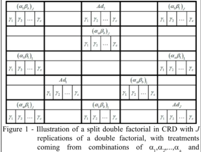
Split double factorial with additional treatment and the post-harvest of Niagara grapes
Texto
Imagem

Documentos relacionados
The probability of attending school four our group of interest in this region increased by 6.5 percentage points after the expansion of the Bolsa Família program in 2007 and
Evaluations of soil characteristics were carried out following the experimental design in split-plots in a factorial 5x5, having the managements considered as the plots and the
compared with the results of the germination test, expressed as percentage of germinated seeds, through a completely randomized design, in a 2 x 4 factorial arrangement (two
A test was conducted in a completely randomized design in split plots with factorial scheme of treatments 5 x 2 x 2, being the parcel two types of microcontroller data
This research had as the main objective to evaluate, in situ , through a randomized, split-mouth and double-blind, cross-over design, the influence of fluoride from
Abstract: The objective of this split-mouth, double-blind, randomized controlled trial was to compare the clinical effect of treatment of 2- or 3-wall intrabony
The aim of this study was to evaluate the efficacy of two desensitizing agents in the reduction of dentin hypersensitivity in a randomized, double-blind, split- mouth
The experimental design was completely randomized in 2 x 4 factorial scheme, involving the application of glyphosate in the plants at pre-harvest and the control (without plant
