Abstract
In this paper, a simplified numerical approach to study the influ-ence of the confinement effect provided by transversal reinforce-ment on the ductility behavior of RC beams in bending is pro-posed. A unidimensional FEM mechanical model coupled to the Mazars’ damage model to simulate concrete behavior was adopted to assess ductility curvatures at the ultimate limit state. The con-finement effect was incorporated to the numerical model through a calibration process of the damage internal parameters, based on the Least Square Method and an analytical law proposed by Kent and Park (1971). Several numerical analyses were carried out consider-ing different designs of RC beams accordconsider-ing to a parametric study varying the neutral axis position, concrete compressive strength and the volumetric transversal reinforcement ratio. The obtained results showed the importance of the amount of transversal rein-forcement on the ductility behavior, increasing the ductility factor even for the cases with inappropriate neutral axis position.
Keywords
RC beams, finite element; ductility; confinement; concrete; damage.
Ductility Analysis of RC Beams Considering
the Concrete Confinement Effect Produced
by the Shear Reinforcement: a Numerical Approach
1 INTRODUCTION
Nowadays, reinforced concrete (RC) structures are largely used in engineering works from small constructions to tall buildings and bridges. The possibility to build any kind of geometry and for-mat for the structural systems have given to reinforced concrete the status of general construction material. The costs associated to the construction of the buildings and other structures are still competitive when compared to several materials. Furthermore, RC as a structural material, espe-cially when used for example in statically indeterminate structures, gives to the elements the
capac-Caio Gorla Nogueira a, * Isabela Durci Rodrigues b
a Department of Civil Engineering, São Paulo State University – UNESP/FEB, Brazil - cgnogueira@feb.unesp.br b Department of Civil Engineering, São Paulo State University – UNESP/FEB, Brazil - isabela.dr@hotmail.com * Corresponding Author
http://dx.doi.org/10.1590/1679-78253904
ity to behave according to the assumptions specified by the designer of the structural system, since the designing and execution of the structure respect the design hypothesis, limitations imposed by the codes and good procedures in situ. Regarding to the RC beams, the most part of these structur-al elements is designed to support bending moments and shear forces that come from the externstructur-al loads. But, in general, the bending moment effects are more important than the shear ones, espe-cially when the beams have higher values of the span-to-depth ratio, in which the shear strains can be neglected and the Euler-Bernoulli’s hypothesis governs the overall structural behavior and main-ly the ultimate strength of those elements.
Among many aspects required in RC beams and slabs design, ductility has become mandatory by the standard codes (ABNT NBR 6118: 2014; EUROCODE 2: 2004; ACI 318: 2002). In this con-text, ductility can be defined as the ability to support large plastic deformations before failure with-out significant resistance loss. The main reasons to consider ductility as a mandatory characteristic in the modern structural design are: ductility prevents brittle ruptures, which is a failure mode that must always be avoided; elements with ductile behavior have higher plastic rotation capacities when compared to brittle elements and contribute to large deformations/displacements before a physic rupture (Ko et al. 2001); ductility of cross sections are essential to provide bending moment redis-tribution along the beam as longitudinal reinforcement steel yields ensuring the redundant behavior of hyperstatic structures (Kara and Ashour 2013). Another important application in which the duc-tility is essential to guarantee safe behaviors of RC structural systems is related to dynamic loads generated by seismic tremors. In such cases, the ductility of the structural elements must be pre-dicted and quantified in a detailed way to avoid severe damage and brittle failures of the buildings (Lopes et. al 2012; Arslan 2012; Demir et al. 2016).
However, the prediction and the assessment of ductility as a single value to describe how ductile or brittle is an element or some cross section is not an easy task. There are several parameters in-teracting each other that influence the ductility at ultimate limit states. Moreover, it is impossible to dissociates ductility from rigidity of a RC element because they are function of almost the same parameters as: longitudinal reinforcement ratio, concrete strength, concrete softening branch in compression, crack pattern development, tension stiffening, bond-slip relationship (Lee and Pan 2003; Oehlers et al. 2009; Lopes et al. 2012). The curvature depends on the material strain levels and their limits. On the other hand, these strain values are function of the neutral axis position, which influences the effective depth and longitudinal reinforcement ratio.
confinement effect of the compressed concrete provided by stirrups and tension stiffening (Oehlers et al. 2013).
Damage models (Mazars 1984; La Borderie 1991; Flores-Lopes 1993; Cervera et al. 1996) have been adopted successfully to represent the rigidity loss of the structural elements as a function of the loading conditions. In the most of damage models, the damage is defined by a scalar parameter that quantifies the local state of degradation and penalizes the material stiffness at that point. To perform the damage assessment, there are several constitutive models with their own assumptions and hypothesis about the starting and evolution of the damage. But as a general approach, damage models depend on the stress/strain state at a point (integration points localized along the finite elements) and an evolution criterion for damage. By adopting damage model approaches, the limi-tation on the EI values and its variation along the structural elements is overcome.
In the context of the absence of explicit quantification methods for ductility, Lee and Pan (2003) proposed an algorithm based on simplified analytical equations to RC beams designing con-sidering that ductility factor as an input data. In their approach, the authors considered the Kent and Park’s (1971) analytical model for concrete in compression to take into account the confine-ment effect caused by the transversal reinforceconfine-ment. Daniell et al. (2008) studied the ductility in RC elements considering the plastic rotation capacity as a measure of ductility and associated it with ability to redistribute bending moments. Arslan (2012) carried out a parametric study varying some parameters listed in the design codes in order to ensure enough ductility for RC structures when subjected to earthquakes.
This paper presents a study about the influence of the confinement effect in RC beams ductility provided by shear reinforcement, considering a numerical approach via FEM. The confinement ef-fect was incorporated to a unidimensional FEM mechanical model through a calibration procedure of the internal damage parameters adopted by the scalar Mazars’ damage model. The calibration was carried out by a Nonlinear Least Square Method based on the Gauss-Newton strategy solution. Therefore, the effect of the confinement was automatically incorporated to the constitutive concrete compression law after concrete reach the stress × strain curve peak. The paper’s main contribution is related to the use of a simplified numerical approach based on the calibration of the internal damage parameters taking into account the confinement effect. If the constitutive law of the mate-rial is known, the proposed procedure can be applied, which gives a general status to the model. A parametric analysis was carried out in a RC beam to study the effect of the confinement on the ductility, varying the neutral axis position, concrete strength and volumetric transversal reinforce-ment ratio.
2 THE MECHANICAL MODEL BASED ON FEM
2.1 Unidimensional Finite Element Approach
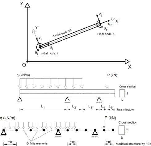
(dof): 2 translational displacements (u and v in x’ and y’ respectively) and 1 rotation ( in z), which implies in the total of 6 dof per element (3 per each node). Nogueira et al. (2013) presented the original formulation of the 1D finite element adopted here, which is based on the traditional displacement approach.
Figure 1: Frame plane 1D finite element and an example of discretization.
2.2 Isotropic Damage Model for Concrete
The effective second order stress tensor ( ) at the point can be defined by:
: (1)
In which: is the linear elastic fourth order constitutive tensor; is the second order strain ten-sor.
After the solution of the linear system of equations derived from the FEM, the strain tensor is achieved based on the nodal displacements for each integration point along the cross section of the
element. Note that in the strain tensor there are the normal ( , , ) and shear ( , , )
components which represent the entire state of strain. As one can define the strain tensor at each point of the element, the damage parameter can also be assessed for each integration point and it is used to evaluate the final effective stress later. Then, for each integration point, the eigenvalues of the strain tensor ( , , ) are obtained to analyze the degradation state as written below:
∗ 0 0 00
0 0 (2)
The damage criterion used to verify the concrete integrity at each integration point can be giv-en by:
, 0 (3)
In which: is the equivalent strain that represents the stretching state at the point; indi-cates the current threshold of the degradation state. In fact, this value controls the size of the
dam-age surface, which expands when the equivalent strain reaches .
In the beginning of the incremental-interactive process, receives the strain corresponding
to the concrete peak stress (ftk) in tension, which is ⁄ . When the criterion described by
Equation 3 is violated, is updated by the last value of the equivalent strain. The equivalent strain assumes the form:
(4)
The equivalent strain takes into account only the positive components of the main strain tensor
∗ because it reflects the hypothesis of the model that is damage is due only by stretching states.
The damage model of Mazars (1984) is defined by two independent damage parameters (DT and DC) to consider the non-symmetric behavior of concrete in tension and compression. After the assessment of each damage parameter, the final value of the damage (D) is given by the linear combination:
(5)
A strategy, proposed by Perego (1990), was developed to evaluate such parameters and adopted in this work. The followed steps are written below and are applicable to each integration point along the cross section of the finite elements:
A) Evaluate the main strain tensor (*); B) Evaluate the main stress tensor (*) by:
∗ : ∗ (6)
A) Split * into two parts, one positive ( ∗) and the other negative ( ∗) by:
∗ ∗ ∗ (7)
B) Evaluate the positive ( ∗) and negative ( ∗) strain tensor by:
∗ : ∗
∗ : ∗ (8)
After these steps, the weight factors can be given by:
∑ ∗
∑ ∗
(9)
In which: corresponds to the inverse of the linear elastic fourth order constitutive tensor;
∗ represents only the positive components of the positive strain tensor ( ∗ ; ∗ represents
only the positive components of the negative strain tensor ( ∗ ; is the strain value correspondent to the total stretching state at the point assuming the form:
∗ ∗ (10)
The independent damage parameters (DT and DC) are functions of the equivalent strain, and a set of internal parameters (AT, BT, AC, BC,) calibrated to represent concrete behavior in ten-sion and compresten-sion observed by uniaxial experimental tests as:
1 1 ̃
1 1 ̃
(11)
Mazars (1984) proposed some limits for these internal parameters based on several experimental analyses as following:
0,7 1,0
1,0 1,5
10 2 10
Finally, the real stress tensor at the point assumes the form:
1 : (13)
It is worthy to mention that the (1 – D) penalizes all the stress components on the stress ten-sor, even the shear stress. Therefore, the isotropic behavior of the damage model still stands over the complete stress tensor.
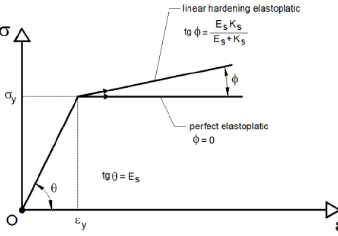
2.3 Elastoplastic Model for Steel
Steel has as main feature, the presence of a plastic behavior after it reaches the yielding stress. It means that in case of an unloading process, at any stage of the analysis, a residual strain appears and cannot be recovered. Therefore, an elastoplastic behavior is observed, in which after yielding there are two possibilities: the perfect elastoplastic way and the elastoplastic with linear isotropic hardening way. In the first on, the normal stress keeps constant equal to the yielding stress until the physical breakage of steel. In the second one, a hardening phase emerges after yielding, in which some loss of stiffness is observed, but the material is still able to resist until the breakage. In the numerical modelling, the mathematical difference between the two approaches is in the plastic coef-ficient of steel (KS). For perfect elastoplastic behavior, KS = 0 and for the elastoplastic with linear hardening, KS 0, varying from 1% to 10% of the steel Young modulus (ES). Figure 2 shows these two approaches for steel modelling adopted in this work. As the longitudinal and transversal rein-forcement are defined by several layers along the cross section and the finite element length, respec-tively, an uniaxial plasticity approach was adopted. In such case, the main objective of the algo-rithm consists in to correct the elastic predictor stress, which is defined only by one value (S) at the reinforcement layer.
The plasticity algorithm to the corrected stress assessment is described below and it is applied to each longitudinal reinforcement layer and stirrups along the element length. The nomenclature i+1 stands for the actual increment and i corresponds to the last converged increment.
A) Evaluate the current strain (i+1) by:
∆ (14)
B) Evaluate the current elastic predictor stress (i+1) by:
(15)
C) Plastic criterion verification (fi+1):
0 (16)
The steel plasticizes if the condition 0 is achieved; on the other hand, the steel remains
elastic. The next steps occur just in case of the plastic criterion is not verified, i.e., if 0. D) Evaluate the current increment of the plastic strain () by:
∆ ∆ (17)
The function sign (.) only takes into account the signal of the stress to differentiate tension and compression layers and assumes the form:
1 → 0
1 → 0 (18)
E) Evaluate the current plastic strain (pi+1) by:
∆ (19)
F) Evaluate the current value for i+1 by:
∆ (20)
G) Evaluate the corrected steel’s Young modulus ( ) by:
(21)
H) Evaluate the corrected stress (i+1) by:
(22)
Note that, the new value of every time plastic strains increase means that the plastic surface size also increases.
If the plastic criterion is not violated, the current stress at the reinforcement remains the same assessed by the elastic predictor in Equation 15. It means that = 0 and there is no plastic strain yet or there is no evolution of the plasticization.
2.4 Shear Resistance Model with Stirrups
In standards approaches of unidimensional FEM, the transversal reinforcement contribution is not take into account. The finite element stiffness matrix is constructed considering the influence of the concrete and longitudinal reinforcement, but none reference is done about the stirrups. It happens because in both cases, concrete and reinforcement bars are subjected by normal stresses acting in X axis (longitudinal direction). But in case of the transversal reinforcement, although the stirrups branches are subjected too by normal stresses, these stresses act in the Y axis (transversal direc-tion). In traditional beams, the transversal normal stress y can be neglected and the stress state at any point has only two components: normal stress x and shear stress xy. Therefore, there is no direct connection between y and the stress acting along the stirrups.
Belarbi and Hsu (1990) carried out experimental tests in T cross section RC beams to observe the stress distribution along vertical stirrups and to assess from what moment the stirrups really contribute to resist shear forces. They observed that the magnitude of the stresses increases from the compressed banzo to tensile banzo, but decreases near the longitudinal reinforcement. It is also observed that the real contribution of the transversal reinforcement occurs after the concrete crack-ing. Before this, only the undamaged concrete and the aggregate interlock for low values of damage support all the shear stresses. Based on this behavior, it was adopted here the alternative model proposed by Nogueira (2010), which considers the presence of the transversal reinforcement by its geometrical rate along the beam and its contribution only after the damage process begins. In this way, the shear reinforcement contribution is linked with the damage model sharing the same crite-rion to starts its effects. As the equivalent strain is defined by the sum of positive components of the strain tensor, damage is associated only to stretching (tension strains). Furthermore, it is con-sidered that in concrete, the opening of diagonal cracks is directly associated to the main tension strain 1. Because of such behavior, it will be assumed that the stirrups strain will be also associated
to 1, but only to the dissipated portion as described below.
After damage beginning, it is considered the split of the strain tensor in two parts: the elastic one (e index) which can be recovered and the damaged one (d index), which is dissipated during the process of damaging evolution.
(23)
In the same way, the real stress tensor at a point can be splitted in an elastic and damaged part as:
Concrete is responsible to resist the first term of the Equation 24. The second term given by
: can be rewritten as:
: : (25)
In which: d is the damaged strain tensor at a point due the evolution of the damage.
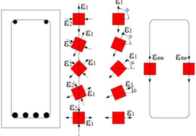
However, as the stirrups are subjected only to normal stresses, the transversal reinforcement strain will be given by the dissipated part of the main tension strain 1, defined by 1d, rotated to the reinforcement direction, which is, in general, vertical. In the same way, the compressed strut in a point will have the same strain of the main compression strain 2. Those values are all assessed in each integration point along the cross section of the elements. Following the observations made by the Belarbi and Hsu (1990) tests, the stirrup’s strain, as depicted in Figure 3, will be the maximum value of 1d rotated to vertical direction along the cross section as:
max sin max sin (26)
In which: is the main direction related to 1.
At the fibers nearby the tension longitudinal reinforcement, the stirrup’s strain will be very low because the main direction for tension is almost zero, which means there will be no transversal component. On the other hand, at the compressed fibers nearby the longitudinal reinforcement, the values of the damage parameter D and the 1 are also very low and offer a tiny contribution for the transversal reinforcement. Therefore, the higher values of the rotated damaged strain will be ad-dressed around the middle of the cross section, but not necessary at its center. This approach to assess the stirrup’s strain considers the nonlinear behavior of the concrete.
Figure 3: Distribution of the main tension strain along the cross section and the adopted stirrup’s strain.
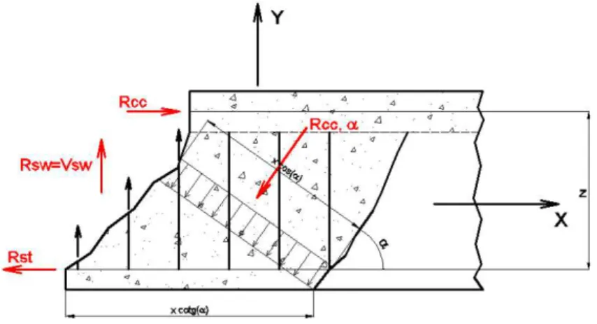
Figure 4: Force distribution for a cracked concrete element.
The forces Rcc and Rst are, respectively, the resultants on the compressed concrete zone and the longitudinal tension reinforcement. The model assumes that the force Rcc, along the compressed strut is already taken into account by the concrete contribution in shear force. Thus, the force in the transversal reinforcement Vsw can be evaluated by the product between the reinforcement area Asw and the stirrup stress sw for each band equal to the effective depth d of the cross section as:
(27)
In which: sw is the geometric transversal reinforcement rate and can be given by ⁄ ; bw
corresponds to the cross section width of the element; sw is the spacing between stirrups.
2.5 Kent and Park’s Confinement Model for Concrete
The original formulation of the Kent and Park (1971) model for concrete in compression was adopt-ed to simulate the confinement effect due to the transversal reinforcement. The model was first developed to be used in compressed elements, but it was already used to study the influence of con-finement in RC beams in bending (Delalibera, 2002; Lee and Pan, 2003). The main purpose of this model is to increase ductility (but not resistance) by considering a soft linear post peak behavior of the compressed concrete, as depicted in Figure 5.
The constitutive law is divided in three parts with the following equations to describe each part: AB: 0,002
2
0,002 0,002 (28)
In which: fc’ is the compressive strength of non-confined concrete in MPa; fc corresponds to the
apparent compressive strength of the confined concrete in MPa; c is the strain of the non-confined
concrete. BC:0,002
1 0,002 (29)
In which: 20c corresponds to the strain of the confined concrete at 0,2fc’; z is the parameter that
defines the slope of the descending branch of the curve and depends on the volumetric transversal reinforcement ratio. The parameter z assumes the form:
0,5 3 0,29 ′
145 1000 34 0,002 (30)
In which: vw is the volumetric transversal reinforcement ratio; bvw is the width of the
confine-ment zone at the cross section in millimeters; svw is the spacing between the stirrups used to confine
the concrete in millimeters.
CD:
0,2 ′ (31)
In the CD branch, it is considered that the structural element has achieved the strain referent to 20% of the maximum concrete strength in tension.
It is worthy to mention that unconfined concrete can also be modeled with the described model by considering vw= 0 and deleting the response beyond C.
2.6 Calibration Technique for Internal Damage Parameters
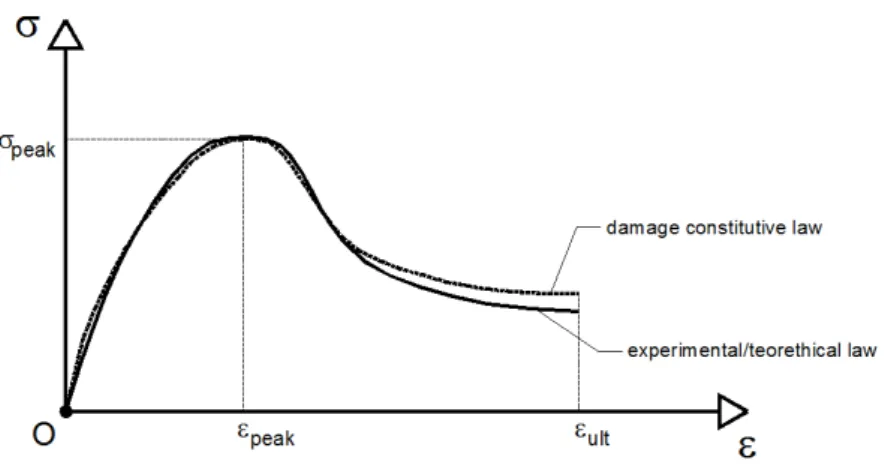
Figure 6: Comparison between idealized (damage constitutive law) and the “real” (experimental/theoretical) behavior.
To achieve this, the problem can be formulated by using the Least Square Method according to:
, 12 , (32)
In which: U and X are, respectively, the parameters set that will not and that will be calibrat-ed; n corresponds to the number of known answers from the experimental data or from the theoret-ical source; f is defined as the local error function and gives the differences between the known and the unknown answers of the experiment. In such case, the problem consists in represent the con-crete behavior, in tension and compression, by the constitutive law proposed by the Mazars’ dam-age model. In the absence of experimental data for several concrete classes of strength, with or without the presence of the confinement effect, theoretical laws in the literature can be used to give the responses in uniaxial tension (T) and compression (C) tests. Thus, the local error functions as-sume the form:
, , 1 ,
, , 1 , (33)
In which: DT and DC are, respectively, the damage parameters for tension and compression
giv-en by Equation 11; E is the concrete Young modulus; T and C are, respectively, the concrete
strain in the uniaxial test for tension and compression. In case of compression, C,known is assessed
by Kent and Park’s model described by Equations 28, 29 and 31. Regarding concrete behavior in tension, the T,known is given by the Figueiras’ constitutive law (1983) or any other law.
To formulate that, a function F(X+H, U) can be approximated by a Taylor’s series expansion:
, , , 12 ,
, 12 (34)
In which: G and Q are, respectively, the gradient and the hessian matrices of the function F; H indicates a descendant direction for F to the minimum point.
The gradient and hessian matrices assume the form:
, …… (35)
,
⋯
⋮ ⋱ ⋮
⋯
(36)
In which: k corresponds to the number of calibrated parameters (in such case k = 2).
In order to simplify the understanding but without loss of generality, the same minimization process can be written using the local error function f. Assuming that f and its derivatives are
con-tinuous in the considered domain, the gradient G and the hessian matrix Q can now be described
as:
,
,
,
,
,
(37)
,
, ,
, , , , , ,
, ,
, , , , , ,
(38)
In which: the , terms are the Jacobean (J) of the function and can be described as:
,
, ,
⋮ ⋮
, , (39)
, , , (40)
, , , , , (41)
To solve the problem proposed by Equation 32, the Gauss-Newton technique was adopted. This
approach uses a linear approximation to function f(X,U) at the neighborhood of point X, which
allows, by an expansion in Taylor’s series, write the value of the f(X+H,U) according to:
, ≅ , , (42)
Replacing Equation 42 in 34, the lagrangean L(H) of the function F can be obtained as:
, ≅ ≅ , , , 12 , , (43)
Therefore, the solution of the problem consists in to find the descendant direction H that min-imizes L(H). The gradient and the hessian considering now the lagrangean are given, respectively, by L’(H) and L’’(H) as:
, , , , (44)
, , (45)
When H is close to zero, L’(H) = F’(H) and the condition of F’(H) = 0 can be replaced by L’(H) = 0. If the columns of the Jacobean matrix are linear independent, than the hessian of the lagrangean L’’(H) is positive-definite, which guarantee that L(H) has a minimum point given by:
0 → , , , , 0 (46)
Finally, the vector H can be assessed by the solution of system:
, , (47)
This an iterative procedure in which at the end of the m-iteration, the vector H is added to the last updated X. This procedure is repeated until the new H is the same as the one obtained at the last iteration. At the end of the calibration process, XC and XT provide the values of the internal damage model (AC, BC) and (AT, BT), respectively.
2.7 Solution of the Nonlinear Problem
was also added to the nonlinear problem. As described by Equation 27, the contribution of the shear reinforcement was only considered for the internal forces assessment, which means that there was no addition of the stirrups contribution on the local stiffness matrix of the elements and, conse-quently, on the global stiffness matrix of the total system. Therefore, a consistent tangent matrix approach was not able to be used and a similar technique was adopted. The stiffness matrix was constructed at the beginning of each iteration, as in the tangent approach, but only considering the contributions of concrete and longitudinal steel. After the evaluation of the damage parameter for each integration point along the cross section height, the influence of the degradation state is taking into account to evaluate the contribution of such integration point at the assessment of the local stiffness matrix for the next iteration. More details about the FEM mechanical model can be found in Nogueira et al. (2013).
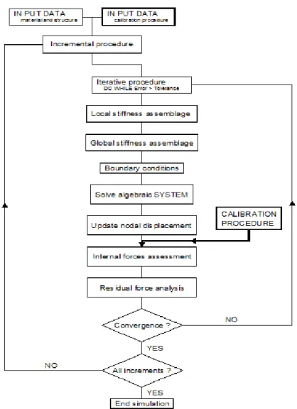
Figure 7 shows a schematic flowchart of the mechanical model with the introduction of the pa-rameters calibration procedure. Some details about the main steps are discussed below.
– IN PUT DATA (material and structure/calibration procedure): the elastic material
proper-ties, loading/displacement parameters and structure information are all described here. Re-garding the calibration procedure, the first trials for the tension and compression parameters of the damage model are given: XC0 = (AC, BC) and XT0 = (AT, BT). The limit value of the strain for each tension and compression is also given for the discretization process to approx-imate the theoretical constitutive law. The number of strain increments is another parameter and it is represented by the n value in Equation 32;
– Local stiffness assemblage: the local stiffness matrix of each finite element [k]FE is given by:
, , , (48)
In which: [k]c, flexure is the contribution of concrete in flexure (bending moment); [k]c, shear is the contribution of concrete in shear; [k]s, longitudinal is the contribution of longitudinal reinforcement. It is worth to mention that the contribution of the shear reinforcement (stirrups) is not considered.
– Global stiffness assemblage: the global stiffness matrix is constructed here by the sum of each element stiffness matrix;
– Internal forces assessment: in this subroutine of the mechanical model, the internal efforts normal force, shear force and bending moment for each finite element node are evaluated considering the updating of damage and plastic strains that may occur along the loading pro-cess. But before such calculations, for each finite element, the damage parameters are cali-brated according to the described procedure in section 2.6. It is evident that if there are no different concrete strengths along the finite element mesh, this procedure can be done only once at the beginning of the internal forces assessment subroutine and keeps constant for all the subsequent steps of the simulation.
With this approach of incremental displacement applied, it is possible to represent the post peak softening branch of the structural behavior of the beams and evaluate the ductility.
3 DUCTILITY OF REINFORCED CONCRETE ELEMENTS
The approach to assess the curvature ductility or also called as ductility factor adopted in this work is based on the one described by Lee and Pan (2003). Hence, the ductility factor () can be given by:
(49)
In which: is the ultimate curvature of the analysed cross section; is the yielding curvature at the same cross section.
defined the ultimate curvature when the compressed strain of the concrete compressed fiber at the
same layer of compressed reinforcement reached the value of 5,0‰. Eurocode 8 and Lopes et al.
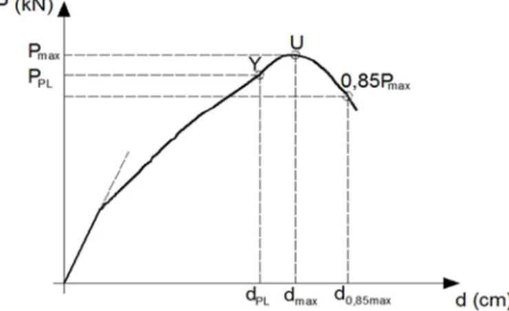
(2012) considered that ultimate curvature is defined by the correspondent curvature at 85% of the resistant cross section bending moment, after the peak of the equilibrium trajectory has be achieved. In this paper, the ultimate curvature was obtained from the correspondent value of ulti-mate bending moment at the analyzed cross section given by the ultiulti-mate load of the whole struc-ture. Figure 8 illustrates the adopted approach. The marks Y and U stand for yielding curvature and ultimate curvature, respectively, while the 0,85Pmax indicates de ultimate curvature considered by Lopes et al. (2012). As a displacement control process over the structure was applied, when the ultimate load is reached, the correspondent curvature at the considered cross section is adopted as the ultimate curvature. In such way, the ultimate curvature does not depend on a specific value of strain in any position of the cross section, which grants to this approach a general aspect. Further-more, the ultimate curvature reflects, at the studied cross section, the global resistance of the con-sidered structural element.
Figure 8: Yielding and ultimate curvature adopted in the study.
4 PARAMETRIC ANALYSIS
To perform the assessment of the ductility factor in reinforced concrete beams, a parametric analy-sis was carried out. The numerical analyses were conducted in order to show the influence of the confinement effect provided by different transversal reinforcement rates over the ductility of the RC beams at the ultimate limit state. Moreover, another question motivated the numerical tests, which was: is there any compromise between longitudinal and transversal reinforcement that influences the ductile behavior of RC beams? To answer these questions the following steps were performed and they are described below.
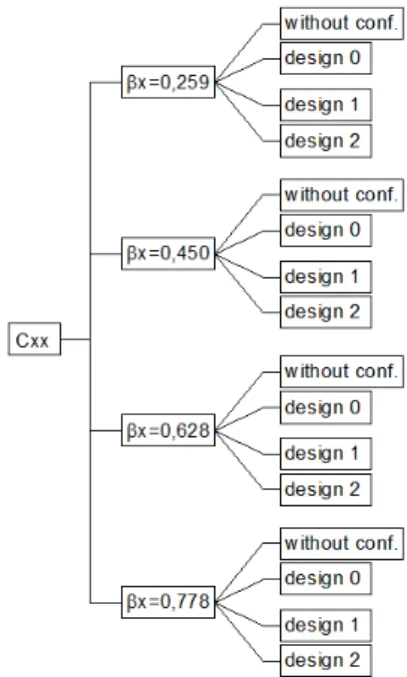
as ABNT NBR 6118, EUROCODE 2 and others), a limitation of the neutral axis position must be imposed to guarantee the ductile behavior of the elements. For example, the Brazilian code (ABNT NBR 6118) defines such limit for x, as 0,450 in case of concretes with characteristic compression strength until 50MPa. Beyond this value, the ductility is impaired and a brittle behavior produced by the concrete crushing may occur, which must be avoided in practice. Then, for each value of x, another four situations were considered regarding the amount of transversal reinforcement to assess the influence of the confinement effect over ductility. The cases “without conf.” and “design 0” have the same volumetric transversal reinforcement rate, but in the first one, there is no confinement effect and in the second one, this effect was taking into account by the Kent and Park’s constitutive law. “Designs 1” and “2” were adopted decreasing the spacing between consecutive stirrups taking as reference those values achieved in “design 0”, by 60% and 30%, respectively. Figure 9 summarizes all the adopted models tested in the parametric analysis. The legend xx indicates 20, 30 and 40 MPa. Therefore, 16 3 = 48 numerical analyses were performed in the ductility study. The results are shown in the section 5.2 of this article.
Figure 9: Flowchart of the parametric analysis for the ductility study.
The mechanical model based on MEF unidimensional approach coupled to all the described nonlinear models for concrete, steel and shear reinforcement were used in the parametric analyses.
5 RESULTS
5.1 RC beams Tested by Ziara et al. (1995)
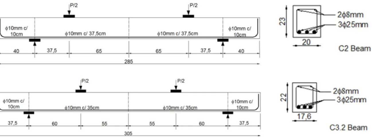
were numerically analysed by Delalibera (2002) and also with the proposed model described in this paper with the same purpose. The confinement effect was simulated by the calibration of the dam-age internal parameters considering the post peak stress-strain curve for concrete in compression according to Kent and Park’s model. The beams are over reinforced and the stirrups were used all around the cross section, discounting only the concrete cover. Figure 10 shows the static scheme and the details of the analysed beam. Table 1 presents the material properties and other adopted parameters.
It was adopted for concrete: Poisson’s ratio of 0,2 and transversal elasticity modulus equals to /2,4. For the steel, it was used a perfect elastoplastic behaviour model. The beams were ana-lysed considering a regular finite elements mesh. For C2 beam, it was adopted 40 elements, in which: 5 elements for each 40 cm, 5 elements for each 37,5 cm and 10 elements on the central span of 130 cm. For C3.2 beam, it was adopted 46 elements, in which: 5 elements for each 37,5 cm, 8 elements for each 60 cm and 10 elements on the central span of 110 cm.
Figure 10: Beams tested by Ziara et a. (1995).
Beam fck (MPa) ftk (MPa) Ec (GPa) fyk (MPa) fywk (MPa) Es (GPa)
C2 30,5 2,05 31 442 442 210
C3.2 19,6 1,53 25 442 442 210
Table 1: Material properties of the beams.
parameter, given by ⁄ , is the specific deformation corresponding to the tensile strength of
concrete. Therefore, to the group of minimum parameters, assume the same values of the ones
presented in Table 2 for C2 and C3.2 beam. The numerical integration was carried out with 6 points of Gauss along the length (PGL) and 20 points of Gauss along the height (PGH) of the finite elements. The loading process was performed with 0,025 cm vertical displacement increments in the central point (middle span).
Beam εd0 AT AC BT BC
C2 with confinement 6,61×10⁻⁵ 0,722 0,863 10987,134 1213,796 C2 without confinement 6,61×10⁻⁵ 0,722 1,788 10987,134 2455,530 C3.2 with confinement 6,12×10⁻⁵ 0,718 0,631 11617,602 1194,646 C3.2 without confinement 6,12×10⁻⁵ 0,718 0,937 11617,602 1902,636
Minimum --- 0,7 1,0 10000,0 1000,0
Table 2: Internal parameters of the damage model.
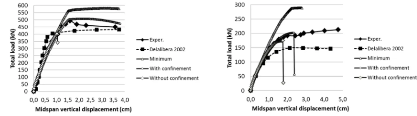
Figure 11 shows the numerical equilibrium path of the C2 and C3.2 beams compared to the ex-perimental and numerical responses obtained by Ziara et al. (1995) and Delalibera (2002), respec-tively. The mechanical model used by Delalibera (2002) was based on MEF with a plane frame finite element of 2 conventional nodes (one in each element’s edge) and 3 degrees of freedom per node (two translations and one rotation). Concrete was represented, in tension and compression, by the constitutive laws of CEB-FIP (1991), while steel was also simulated with elastoplastic behav-iour. For the confined concrete, Delalibera (2002) adopted the model proposed by Saatcioglu and Razvi (1992), which changes the uniaxial behaviour of concrete on the confined zone by the stir-rups.
Three set of damage parameters were used to simulate these beams with the proposed mechani-cal model: minimum, with and without confinement.
Figure 11: Equilibrium path for C2 and C3.2 beams.
Beam Ultimate load values (kN) / Bias factor (Pu,num/Pu,exp)
Experimental Delalibera (2002) Minimum With confinement Without confinement C2 489,3 446,6 /0,91 578,9 / 1,18 506,2 / 1,03 403,2 / 0,82 C3.2 216,1 149,5 / 0,69 288,6 / 1,36 200,9 / 0,93 175,2 / 0,83
Table 3: Ultimate load and bias factor values.
The results show the sensitivity of the mechanical responses when the internal damage parame-ters are modified. The set of minimum parameparame-ters proposed by Mazars (1984) as one can see, on both beams, was not able to adequate represent the equilibrium path of the beams, resulting in high ultimate load values. In both beams, the developed mechanical model represented with good agree-ment the most part of the experiagree-mental response, especially in the case when confineagree-ment was tak-ing into account, even when the confinement effect created by stirrup reinforcements was indirectly considered through the calibration of the damage parameters. In the response without confinement, after the most compressed concrete fibres reached the compressive strength, it was observed a quickly decrease in compression stress even for small values of strain. It means that the confinement can provide more ductility associated with some resistance for concrete in compression after peak.
In the C2 beam, the ultimate load assessed by the mechanical model with confinement was al-most equal to the experimental value. After the peak, the model still was able to represent the sof-tening branch of the equilibrium path. However, in the C3.2 beam, the ultimate load was also well represented, but a more brittle failure was observed with the numerical approach. The high value of longitudinal reinforcement rate associated with the low value of concrete strength (19,6 MPa) re-sulted, with the used damage model, in a numerical brittle failure behaviour.
5.2 Ductility Study
In this example, an isostatic simply supported reinforced concrete beam subjected to a vertical load at midspan was analyzed to quantify the ductility in ultimate limit state for different designs. Fig-ure 12 shows the geometry of the beam and the finite element mesh adopted in the analyses. It was adopted 40 1D finite elements with the same length. For the nonlinear process of solution, the nu-merical integration was carried out with 6 PGL and 20 PGH for each finite element. The loading process was performed with 0,025 cm vertical displacement increments in the central point (middle span). In all cases, the RC beams were designed considering Pk = 30 kN.
Figure 12: RC beam analyzed for the ductility study: dimensions in centimeters.
fck
(MPa) βx
H (cm)
As (cm2)
Without shear
reinforcement Design 0 Design 1 Design 2
20
0,259 40 2,95 Asw = 0 ϕ5mm c/20cm:
1,96 cm2/m ϕ
5mm c/12cm: 3,27 cm2/m ϕ
5mm c/6cm: 6,54 cm2/m
0,450 33 4,07 Asw = 0 ϕ5mm c/17cm:
2,31 cm2/m
ϕ5mm c/10cm: 3,74 cm2/m
ϕ5mm c/5cm: 7,14 cm2/m
0,628 30 5,03 Asw = 0 ϕ 5mm c/15cm:
2,61 cm2/m
ϕ5mm c/9cm: 4,36 cm2/m
ϕ5mm c/4,5cm: 8,73 cm2/m
0,778 28 5,84 Asw = 0 ϕ 5mm c/14cm:
2,81 cm2/m
ϕ5mm c/8,5cm: 4,62 cm2/m
ϕ5mm c/4cm: 9,82 cm2/m
30
0,259 34 3,62 Asw = 0 ϕ5mm c/18cm:
2,18 cm2/m
ϕ5mm c/10,5cm: 3,74 cm2/m
ϕ5mm c/5,5cm: 7,14 cm2/m
0,450 28 4,99 Asw = 0 ϕ5mm c/14cm:
2,81 cm2/m
ϕ5mm c/8,5cm: 4,62 cm2/m
ϕ5mm c/4cm: 9,82 cm2/m
0,628 25 6,17 Asw = 0 ϕ5mm c/12cm:
3,27 cm2/m ϕ
5mm c/7cm: 5,61 cm2/m ϕ
5mm c/3,5cm: 11,22 cm2/m
0,778 24 7,16 Asw = 0 ϕ5mm c/11cm:
3,57 cm2/m ϕ
5mm c/6,5cm: 6,04 cm2/m ϕ
5mm c/3,5cm: 11,22 cm2/m
40
0,259 30 4,18 Asw = 0 ϕ5mm c/15cm:
2,62 cm2/m
ϕ5mm c/9cm: 4,36 cm2/m
ϕ5mm c/4,5cm: 8,73 cm2/m
0,450 24 5,76 Asw = 0 ϕ5mm c/12cm:
3,27 cm2/m
ϕ5mm c/7cm: 5,61 cm2/m
ϕ5mm c/3,5cm: 11,22 cm2/m
0,628 22 7,12 Asw = 0 ϕ5mm c/10cm:
3,93 cm2/m
ϕ5mm c/6cm: 6,54 cm2/m
ϕ5mm c/3cm: 13,09 cm2/m
0,778 21 8,26 Asw = 0 ϕ5mm c/10cm:
3,93 cm2/m
ϕ5mm c/6mm: 6,54 cm2/m
ϕ5mm c/3cm: 13,09 cm2/m Table 4: Adopted values for the parametric study.
transver-sal reinforcement (Asw) for each resistance concrete class (fck). The RC beams were designed to shear forces using the model II of the ABNT NBR 6118 (2014), considering the inclination of 30º with horizontal for the compression struts. Thereafter, design 0 was obtained adopting the maxi-mum value of distance between stirrups allowed by the Brazilian standard, while designs 1 and 2 were defined considering 60% and 30% of that maximum distance between stirrups, respectively.
Table 5 shows the mechanical properties of concrete used in the analyses. For the steel, in all case it was adopted yielding stress of 435 MPa, longitudinal elasticity modulus of 210 GPa and perfect elastoplastic behaviour.
fck (MPa) fctk (MPa) Ec (MPa) Poisson Gc (MPa)
20 1,55 25040 0,20 10435
30 2,03 30670 0,20 12780
40 2,45 35417 0,20 14757
Table 5: Concrete properties.
The Mazars’ damage parameters (AC, BC, AT, BT) for concrete were obtained by calibration process, considering the constitutive laws of Kent and Park (1971) and Figueiras (1983) for com-pression and tension, respectively. Because of the calibration, the confinement effect was represent-ed by the damage model according to the transversal reinforcement volumetric ratio. To illustrate some values, Table 6 presents the damage parameters obtained for each transversal reinforcement design considering all the concrete resistance classes, only for the design with βx = 0,259. For the other values of the neutral axis relative position, the same method was applied to get the damage parameters. In the “Without shear reinforcement” case there is no confinement effect in the com-pressed concrete.
fck (MPa) Stirrups AC BC AT BT
20
Without shear reinforcement 0,973 1923,668 0,720 11562,811
Design 0 0,839 1661,882 0,720 11562,811
Design 1 0,775 1520,801 0,720 11562,811
Design 2 0,704 1348,268 0,720 11562,811
30
Without shear reinforcement 1,747 2431,449 0,723 11026,252
Design 0 1,178 1775,246 0,723 11026,252
Design 1 1,028 1537,857 0,723 11026,252
Design 2 0,923 1347,658 0,723 11026,252
40
Without shear reinforcement 2,809 2836,434 0,726 10684,905
Design 0 1,391 1732,878 0,726 10684,905
Design 1 1,210 1492,230 0,726 10684,905
Design 2 1,092 1314,011 0,726 10684,905
Table 6: Calibrated damage parameters for x = 0,259.
rein-forcement yielding. It indicates a ductile behaviour only by changing the amount of longitudinal reinforcement according to the neutral axis position, which stands for the ductility mentioned in the standard codes (comparison between the black curves). However, it was verified that is possible to increase the ductility on the ultimate limit state by making some changes in the stirrups design. In such cases, a bigger extension of the yielding plateau was achieved when the transversal reinforce-ment volumetric ratio was also increased, by closing the stirrups each other. The green curves indi-cate the higher value of the ductility compared to those in black ones for the same neutral axis po-sition. Even for βx = 0,778 it was observed a significant increase in the ductility of the beam. The same behaviour was achieved for the other values of the βx. But, it is worthy to mention that the decreasing of the stirrups spacing provided much more ductility for lower values of the neutral axis position, which can be seen by the large extensions of the yielding plateau. In general, for C30 and C40 concrete resistance classes, the same behaviour was observed concerning the ductility as a func-tion of βx and amount of transversal reinforcement.
Figure 13: Bending moment curvature relationship at midspan cross section: different shear reinforcement.
Without shear reinforcement Design 0
Design 1 Design 2
Figure 14: Bending moment curvature relationship at midspan cross section: different neutral axis position.
The Figure 15 shows the assessed values of the ductility factor for all combinations of the neu-tral axis position and transversal reinforcement considering the confinement effect for each concrete resistance class. In all the analyzed cases, the confinement effect provided by the stirrups and their different designs increased the ductility of the RC beams. When the spacing between stirrups de-creases, the confinement of the compressed zone in concrete inde-creases, making that the compressive stress at the post-peak also increases compared to the same values without the effect of the con-finement. In such cases, the RC beams can support more loading before the rupture is reached, which means an improvement on the ductility.
Another aspect that deserves to be discussed is the high efficiency of the stirrups design, in ad-dition with the low values of the neutral axis position. As one can see in Figure 15, for lower values
of βx, such as 0,259, the influence of the confinement was expressive compared to the performance
C20 C30
C40
Figure 15: Evolution of the ductility for each concrete resistance class.
Finally, the last aspect to be commented is the influence of the confinement over the different resistance classes of the concrete. The confinement effect, provided by the large values of the trans-versal reinforcement, was more significant in the beams belonged to C40 class than those belonged to C20 for the same relative neutral axis position. It means that in cases of concretes with high resistance, the transversal reinforcement design can be more effective than the neutral axis position when ductility is desired.
Figures 16 to 18 illustrate the relationship between the reinforcement rates and ductility factor for all concrete resistance classes.
Figure 17: Longitudinal and transversal reinforcement rates ductility factor: C30
Figure 18: Longitudinal and transversal reinforcement rates ductility factor: C40.
Regarding to the tension longitudinal reinforcement, the ductility factor increases as amount of reinforcement decreases. Therefore, ductile behaviors are achieved with low values of neutral axis position. When the confinement effect is taking into account, the same behavior is observed, but the ductility is significantly improved in such cases, especially for high resistance concretes (C40).
On the other hand, because of the confinement effect, the ductility factor increases as amount of transversal reinforcement also increases. At least for the analyzed cases, it was observed that the inclination of the curves regarding the horizontal axis shows the influence of the volumetric trans-versal reinforcement rate over the ductility of the beams. Note that such influence also depends on the neutral axis position. Thus, high values of transversal reinforcement in addition with low values of neutral axis position provide the better combination for the ductility at the ultimate limit state.
6 CONCLUSIONS
in compression able to consider such effect. The Kent and Park’s law was adopted in which the confinement effect is described depending on the volumetric transversal reinforcement rate at the post peak portion of the stress strain relationship. Therefore, this module was implemented to the existent model coherently with the shear resistance model already working in the program. After that, the analyses were carried out for a generic isostatic RC beam to study the effect of the con-finement on the ductility behavior of the beam. Some important points observed along the tests will be following discuss:
– The coupling of the existing mechanical model and the new module for calibration of the
damage parameters worked very well and showed complete stability along the nonlinear solu-tion process. When the beams tested by Ziara et al. (1995) were analyzed, the calibrated set of parameters were able to better represent the equilibrium trajectory of the beam than the minimum set proposed by Mazars (1984). Therefore, the results emphasize the importance of a proper definition of the damage parameters to simulate RC elements. With the developed calibration process and the knowledge of the constitutive law capable of to incorporate a de-sired effect, the numerical procedure can be applied to study the overall structure behavior;
– The influence of the longitudinal reinforcement on ductility is defined by the relative neutral axis position along the cross section of the element. For lower values of neutral axis position, the RC beams have higher cross section heights and, consequently, lower longitudinal rein-forcement rates, which grant more ductility to these beams at the ultimate limit state. When the concrete resistance increases, the amount of longitudinal reinforcement required to main-tain the same ductility also increases. Therefore, it was observed a direct dependence between the ductility factor and the longitudinal reinforcement rate;
– Regarding the transversal reinforcement, the confinement effect on the compressed zone of
the cross section provided by this kind of reinforcement influences significantly the ductility. As the volumetric transversal reinforcement rate increases, the confinement effect also in-creases providing an extension of the ductile plateau, which means an improvement of the ductility factor. So, answering the proposed question written in section 4 of this paper: yes, there is an interaction between longitudinal and transversal reinforcement that influences ductility. High values of shear reinforcement coupled to low values of longitudinal reinforce-ment give the better combination for ductility. However, more tests must be carried out, es-pecially the experimental ones to complete finish the research.
Acknowledgements
To FAPESP process 2016/14450-6 for the financial support of this project and to State University of São Paulo – UNESP.
References
ABNT NBR 6118 (2014). Design of concrete structures: procedure, Rio de Janeiro, Brazil.
ACI Committee 318 (2002). Buildings code requirements for structural concrete, Farmington Hills, Michigan – American Concrete Institute.
Arslan, M.K., (2012). Estimation of curvature and displacement ductility in reinforced concrete buildings, KSCE Journal of Civil Engineering 16(5): 759-770.
Belarbi, A. and Hsu, T.T.C., (1990). Stirrup stresses in reinforced concrete beams, ACI Structural Journal 87(5): 530-538.
CEB-FIP Model Code 1990: final draft (1991). Bulletin d’Information, Paris, July 203-205.
Cervera, M., Oliver, J. and Manzoli, O.L., (1996). A rate-dependent isotropic damage model for the seismic analysis of concrete dams, Earthquake Engineering and Structural Dynamics 25: 987-1010.
Delalibera, R.G., (2002). Análise teórica e experimental de vigas de concreto armado com armadura de confinamento, Dissertação de Mestrado, Escola de Engenharia de São Carlos, Universidade de São Paulo.
Daniell, J.E., Oehlers, D.J., Griffith, M.C., Mohamed Ali, M.S. and Ozbakkaloglu, T., (2008). The softening rotation of reinforced concrete members, Engineering Structures 30: 3159-3166.
Demir, A., Caglar, N., Ozturk, H. and Sumer, Y., (2016). Nonlinear finite element study on the improvement of shear capacity in reinforced concrete T-sections beams by an alternative diagonal shear reinforcement, Engineering Structures 120: 158-165.
EUROCODE 2 (1992). Design for concrete structures – Part 1: General rules and rules for buildings, Brussels, Bel-gium.
EUROCODE 8 (2004). Design of structures for earthquake resistance – Part 1: General rules, seismic actions and rules for buildings, Brussels, Belgium.
Figueiras, J.A., (1983). Ultimate load analysis of anisotropic and reinforced concrete plates and shells, Ph.D. Thesis, Department of Civil Engineering, University College of Swansea.
Flores-Lopes, J, (1993). Modelos de daño concentrado para la simulación numérica del colapso de pórticos planos, Revista Internacional de Métodos Numéricos para Cálculo y Diseño em Ingeniería 9(2): 123-139.
Kara, I.F. and Ashour, A.F., (2013). Moment redistribution in continuous FRP reinforced concrete beams, Construc-tion and Building Materials 49: 939-948.
Kent, D.C. and Park, R., (1971). Flexural members with confined concrete, ASCE Proceedings 97(ST7): 1969-1990. Ko, M.Y., Kim, S.W. and Kim, J.K., (2001). Experimental study of the plastic rotation capacity of reinforced high strength concrete beams, RILEM Materials and Structural Journal 34: 302-311.
La Borderie, C., (1991). Phenomenes unilateraux dans un materiau endommageable: modelisation et application a l’analyse de structures en béton, These de Doctorat (in french), Universite Paris, France.
Lee, T.K. and Pan, A.D.E., (2003). Estimating of relationship between tension reinforcement and ductility of rein-forced concrete beams sections, Engineering Structures 25: 1057-1067.
Lopes, A.V., Lopes, S.M.R. and Carmo, R.N.F., (2012). Effects of the compressive reinforcement buckling on the ductility of RC beams in bending, Engineering Structures 37: 14-23.
Mazars, J., (1984). Application de la mechanique de l’endommagement au comportement non lineaire et à la rupture du béton de structure, These de Doctorat (in french), Universite Paris, France.
Nogueira, C.G., (2010). Desenvolvimento de modelos mecânicos, de confiabilidade e de otimização para aplicação em estruturas de concreto armado, Ph.D. Thesis (in portuguese), Escola de Engenharia de São Carlos, Universidade de São Paulo.
Nogueira, C.G., Venturini, W.S. and Coda, H.B., (2013). Material and geometric nonlinear analysis of reinforced concrete frames structures considering the influence of shear strength complementary mechanisms, Latin American Journal of Solids and Structures 10: 953-980.
Oehlers, D.J., Visintin, P., Haskett, M. and Sebastian, W.M., (2013). Flexural ductility fundamental mechanisms governing all RC members in particular FRP RC, Construction and Building Materials 49: 985-997.
Perego, M, (1990). Danneggiamento dei material lapidei: leggi constitutive, analisis per elementi finiti ed applicazio-ni, Tesi di Laurea (in italian), Politecnico di Milano, Anno Accademico.
Pituba, J.J.C, (2003). Sobre a formulação de um modelo de dano para o concreto, Ph.D. Thesis (in portuguese), Escola de Engenharia de São Carlos, Universidade de São Paulo.
Saatcioglu, M. and Razvi, S.R., (1992). Strength and ductility of confined concrete, ASCE Journal of Structural Engineering 118(6): 1590-1607.