of Chemical
Engineering
www.scielo.br/bjcePrinted in BrazilVol. 35, No. 01, pp. 265 – 274, January – March, 2018
* Corresponding Author. Moisés A. Marcelino Neto. E-mail: [email protected]; Phone/Fax: +55 41 33104907 dx.doi.org/10.1590/0104-6632.20180351s20160489
AN EXAMINATION OF THE PREDICTION OF
HYDRATE FORMATION CONDITIONS IN THE
PRESENCE OF THERMODYNAMIC INHIBITORS
Carollina de M. Molinari O. Antunes
1, Celina Kakitani
1,
Moisés A. Marcelino Neto
1,*, Rigoberto E. M. Morales
1and Amadeu K. Sum
2 1 Multiphase Flow Research Center (NUEM), Post-graduate Programme in Mechanical and Materials Engineering (PPGEM),Federal Technological University of Paraná (UTFPR), Curitiba, PR, Brazil
2 Chemical & Biological Engineering Department, Colorado School of Mines, Golden, CO, USA
(Submitted: January 27, 2016; Revised: October 25, 2016; Accepted: November 6, 2016)
Abstract – Gas hydrates are crystalline compounds, solid structures where water traps small guest molecules, typically light gases, in cages formed by hydrogen bonds. They are notorious for causing problems in oil and gas production, transportation and processing. Gas hydrates may form at pressures and temperatures commonly found in natural gas and oil production pipelines, thus causing partial or complete pipe blockages. In order to inhibit hydrate formation, chemicals such as alcohols (e.g., ethanol, methanol, mono-ethylene glycol) and salts (sodium, magnesium or potassium chloride) are injected into the produced stream. The purpose of this work is to briefly review the literature on hydrate formation in mixtures containing light gases (hydrocarbons and carbon dioxide) and water in the presence of thermodynamic inhibitors. Four calculation methods to predict hydrate formation in those systems were examined and compared. Three commercial packages (Multiflash®, PVTSim® and CSMGem) and a hydrate prediction routine in Fortran90 using the van der Waals and Platteeuw theory and the Peng-Robinson equation of state were tested. Predictions given by the four methods were compared to independent experimental data from the literature. In general, the four methods were found to be reasonably accurate. CSMGem and Multiflash® showed the best results.
Keywords: Hydrates, Inhibitor, Prediction, Commercial Packages, Hydrate Routine
INTRODUCTION
Gas hydrates are ice-like, crystalline molecular structures which consist of two groups of components: host and guest molecules. The host molecule is water, whose hydrogen bonds form structures that trap guest molecules under suitable pressure and temperature conditions (Sloan
and Koh, 2008). Hydrates are one of the main flow
assurance problems faced by the oil and gas industry. Once hydrates form, they may agglomerate and produce plugs
that either impair or interrupt the flow in the pipelines,
bringing production to a halt in the latter case. This can occur in gas, gas/condensate, and oil production lines.
Amongst the techniques aimed at preventing hydrate formation, removing the free and dissolved water from
the fluids to be transported is the most reliable one, albeit
unfeasible in many situations. Keeping high temperatures and low pressures so that hydrates do not form is another
strategy. However, in most offshore operations, hydrate
formation is controlled by the injection of a thermodynamic hydrate inhibitor, such as alcohols (e.g., ethanol, methanol, mono-ethylene glycol, etc) and salts (e.g., sodium, potassium or calcium chloride). The prevention of hydrate formation and the safe removal of hydrate plugs incur high costs, raise safety concerns and are well-known deepwater
Amongst the common gases produced in the petroleum industry, methane, ethane, isobutane, propane, nitrogen,
hydrogen sulfide and carbon dioxide are all hydrate formers
(Carroll, 2004). It is well-known that carbon dioxide (CO2) is one of the most common non-hydrocarbon gases found in petroleum reservoirs. In addition, most of the Pre-Salt
fields in Brazil hold a significant amount of CO2, as high as
80% (Melo et al., 2011; Jahn et al., 2012). The pressure and temperature conditions in deepwater petroleum production
(as that found in Pre-Salt fields) are very favourable to
hydrate formation. Thus, both experimental and theoretical studies on hydrate formation, especially when high carbon dioxide contents are present, are important to the oil and gas industry.
Knowing and understanding the role of the pressures
and temperatures in gas hydrate formation is the first step
in controlling hydrate formation. A number of commercial simulators can predict the pressure/temperature conditions that favour hydrate formation. These simulators may use
different thermodynamic models, especially when it comes
to the calculation of the chemical potential of the aqueous
and vapour phases, the effect of hydrocarbons of higher
molecular weights, the impact of hydrate inhibitors, and the equation of state to obtain the fugacities of each component in each phase. A solid understanding of the models used in the available simulators is required to assess the quality of the results given by those simulators as far as the hydrate formation is concerned.
Only a few studies in the literature present a comparative assessment of models/simulators for hydrate prediction. Carroll (2004) examined and compared seven methods for predicting hydrate formation in mixtures containing
hydrogen sulfide. For the set of data examined (125
experimental points), the computer methods CSMHYD and Equi-Phase showed to be reasonably accurate. The authors concluded that these two methods were able to predict the hydrate formation temperature to within 1.7°C in 90% of the cases. Ballard and Sloan (2004) compared the predictions from CSMGem, the hydrate program from the Colorado School of Mines, with CSMHYD (predecessor to CSMGem), and three commercial hydrate prediction
programs (DBRHydrate, Multiflash®, and PVTsim®). The
comparisons were split into two categories for hydrate formation temperatures and pressures, uninhibited and thermodynamically inhibited systems. The authors concluded that all simulators fared favourably, giving results within about 1°C.
In this work, motivated by the high concentration
of carbon dioxide in the Brazilian Pre-Salt fields, we
compared the performance of four simulators to predict the hydrate phase equilibrium in systems containing carbon dioxide and light hydrocarbons, including systems with alcohols and salts (thermodynamic hydrate inhibitors). Due to the importance of high carbon dioxide content systems and the need to have reliable predictions of hydrate phase
equilibria with and without thermodynamic inhibitors, this study gives a critical evaluation of the simulators.
The objective of this work is to briefly review the
literature on hydrate formation in mixtures containing carbon dioxide and light hydrocarbons in the presence of thermodynamic inhibitors. Four simulators that predict hydrate formation for these systems are examined and
compared here: three commercial products (Multiflash®,
PVTsim® and CSMGem) and an in-house hydrate
prediction program that uses the van der Waals and Platteeuw model (van der Waals and Platteeuw, 1959) coupled with the Peng-Robinson equation of state (EoS) (Peng and Robinson, 1976). The purpose is to compare hydrate prediction programs for the hydrate formation pressure at inhibited and uninhibited conditions, focusing mainly on systems containing carbon dioxide. In this work, the evaluated experimental data involved pure CO2 hydrates, CO2-rich (>90 mol %) gas mixtures and also gas mixtures where CO2 is considered a contaminant (<3 mol %), such as in natural gas compositions. The hydrate thermodynamic inhibitors investigated were alcohols and salts.
CALCULATION METHODS
The hydrate prediction program comparisons are divided into two categories for hydrate formation pressure: (1) uninhibited systems, and (2) thermodynamically inhibited systems. These two categories are, in turn, divided into two subcategories: single/simple hydrate (only one guest) and more than one guest or mixture of gases.
Four simulators for predicting hydrate formation are considered:
1. CSMGem from the Colorado School of Mines (version 1.10, release date January 1, 2007)
2. Multiflash® from Infochem/KBC Advanced Technologies
(DLL version 4.4.13)
3. PVTsim® from Calsep A/S (revision 1.2.40 flexlm
version)
4. Hydrate model from NUEM/Federal Technological University of Parana
The first three simulators (CSMGem, Multiflash® and
PVTsim®) are based on rigorous thermodynamic models.
They simulate hydrate formation conditions for gas and oil mixtures and can deal with the most commonly used hydrate thermodynamic inhibitors (methanol, ethanol, glycols, and salts). If the aqueous phase contains salts, the
influence of the salts on the hydrate formation conditions
NUEM/UTFPR Hydrate Model
Kakitani (2014) implemented a model to predict the hydrate equilibrium formation. The basic model assumption relates to the chemical potential of water. At equilibrium, the chemical potential must be the same in all existing phases, that is,
(1)
where superscript H refer to the hydrate phase, L to the liquid phase, V to the vapour phase, and the subscript w to the water.
The chemical potential of the water in the liquid phase is obtained from classical thermodynamics as
(2)
where f is the fugacity and the superscript 0 refers to a reference state for water.
The water chemical potential in the hydrate phase was obtained from statistical thermodynamics, namely from the van der Waals and Platteeuw (1959) model, as:
(3)
where the superscript βrefers to a hypothetical phase in
a crystalline configuration with empty water cavities, vi
is the number of cavities of type i per water molecule in the hydrate structure and Yki is the fractional occupancy of component k in cavity type i. In this work, the water chemical potential in the vapour phase was not considered since it was assumed that the solubility of water in the vapour is negligible.
Substituting Eqs. (2) and (3) in (1), and applying the Gibbs-Duhem equation, the equation in terms of measurable variables (p, T) becomes:
H L V
w w w
µ
=
µ
=
µ
0
0
ln
L
L w
w w L
f
RT
f
µ
=
µ
+
ln 1
Hw w i ki
i k
RT
v
Y
β
µ
=
µ
+
−
∑
∑
(
)
( )
0
0
0
0 0
0 2
0
ln
ln 1
T
p T
T L
w i ki
i k
T
H
c dT
V
dT
p
p
a
v
Y
RT
RT
RT
µ
∆
+ ∆
∆
−
+
∆
−
=
−
−
∫
∑
∑
∫
(4)where Δμ0, ΔH0 and ΔV0 are the differences in chemical
potentials, molar enthalpies and molar volumes, respectively, between water in empty cavities and the reference state. These properties are tabulated in Table 1.
The heat capacity difference between the empty hydrate lattice and pure liquid water phase is given by Δcp = -37.32+0.179(T-T0) according to Chapoy et al. (2012).
Equation (4) must be solved so as to obtain the state
conditions for the hydrate equilibrium formation for a specific
gas (guest). As Eq. (4) is implicit in pressure (p), an iterative process to calculate the equilibrium pressure at any temperature (T) becomes necessary. This equation was implemented as a Fortran90 code and solved by means of the secant method.
Fugacities of the gaseous components are calculated by the Peng and Robinson (1976) equation of state. Fugacities of water in the liquid phase are calculated by
(5)
From the definition of activity coefficient in a liquid
mixture,
(6)
where xw is the mole fraction of the free water available to form hydrates.
Thus, the water fugacity in a liquid mixture in the presence of an inhibitor is:
(7)
If there is no addition of inhibitors, that is, for an
ideal solution, the activity coefficient is unity and the
water fugacity is proportional to the mole fraction of the free water. If the solution is non-ideal, as is the case for
mixtures with alcohol and salts, the activity coefficient
must be calculated. Moreover, the gas solubility in water (xg = 1 − xw) is usually considered to have no influence on the activity coefficient of water. As the gas solubility in
the liquid water increases, the mole fraction of the water decreases, thus decreasing its activity.
In this work, two types of thermodynamic inhibitors were considered: alcohols and salts. Salts dissolve in
water and form an electrolyte solution, which is different
from the alcohol and water solution. This fact impacts
the water activity coefficient calculation and in this work two activity coefficient models were used depending
on the type of inhibitor. For alcohols, the water activity
coefficient was calculated using the UNIQUAC model
(Abrams and Prausnitz, 1975). For electrolytes, the water
0
ˆ
ˆ
ww w
f
a
f
=
ˆ
w ww
a
x
γ
=
0
ˆ
w w w w
activity coefficient was calculated using the Debye-Hückel
model (Sander et al., 1986).
Sloan and Koh (2008) proposed the use of the Krichevsky and Kasaranovsky (1935) correlation to calculate the mole fraction of the water. This correlation is used in this work. It follows,
(8)
where Vis the gas molar volume in infinite dilution and H is the Henry constant that can be calculated by the following equation:
(9)
In this equation, H0,1,2,3...are the specific constants of each gas or guest. These particular constants were obtained from Sloan and Koh (2008).
The fractional occupancy of component k in the cavity type i, (Yki), is described by:
(10)
where Cki is the Langmuir constant for the gas component k
in cavity type i and fk is the fugacity of the component k in the vapour phase. Parrish and Prausnitz (1972) improved the van der Waals and Platteeuw (1959) and McKoy and Sinanoglu (1963) models. They used the following expression to calculate the Langmuir constants:
(11)
where ω(r) is the intermolecular potential between the
guest and the host, k is the Boltzmann constant, and r is the radial position. Parrish and Prausnitz (1972) and McKoy and Sinanoglu (1963) used the Kihara potential to account for the intermolecular potential.
Munck et al. (1988) and Parrish and Prausnitz (1972) proposed the following expression to calculate the Langmuir constants:
(12)
where Aki and Bki are tabulated values adjusted to experimental data.
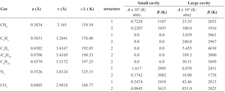
In this study, the Langmuir constants were calculated in two ways: using the expression proposed by Munck et al. (1988) and Parrish and Prausnitz (1972) (Eq. 12) and using the Kihara potential (Eq. 11) (McKoy and Sinanoglu, 1963). Table 2 shows the Kihara parameters (a, σ, ɛ/k) and parameters A and B (Munck correlation) for the calculation of Langmuir constants used in this work.
For further details about the model and solution algorithm in the implementation, see Kakitani (2014).
DATA ANALYSIS
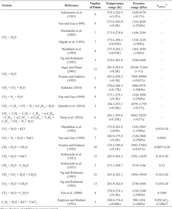
Predictions given by the four methods were compared against experimental data from the literature. Table 3 shows the investigated systems and the related literature. All the experimental points investigated are below the upper quadruple point, that is, they are in the aqueous liquid-hydrate-vapour (Lw-H-V) equilibrium. No data above the upper quadruple point were considered. In this study, a total of 225 experimental points are examined.
The four methods discussed above were used to
calculate the hydrate equilibrium pressure, at a fixed
temperature, point-by-point and the results are presented in terms of a percentage average absolute deviation, AARD,
(13)
where n is the number of points, piexp is the experimental
pressure and pical is the calculated pressure for point i.
RESULTS AND DISCUSSION
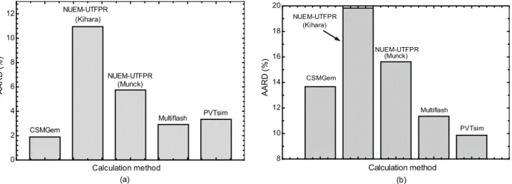
Each of the calculation methods discussed above was used to estimate the hydrate equilibrium pressure for each of the data sets. Figure 1 shows the AARDs of each calculation method for uninhibited systems. Figure 1(a) is for a single guest and Figure 1(b) is for more than one guest. Figure 1(a) and 1(b) suggest that one can expect the incipient hydrate pressure formation to be predicted within 11% and 20% accuracy for a single guest and for more than one guest, respectively. However, from Fig. 1(b), it is apparent that more reliable thermodynamic data are needed for systems with more than one guest. The AARDs for
CSMGem, Multiflash®and PVTsim® are about 2%, 3% and
3.5% for a single guest, respectively, and 13.5%, 11% and 10% for systems with more than one guest, respectively. It can be observed that, for systems with a single guest and with more than one guest, the NUEM-UTFPR model that uses the Munck correlation performed better than the model that uses the Kihara potential.
Table 1. Physical properties of sI hydrate (Sloan and Koh, 2008). Δμ0 (J·mol
-1) 1263
ΔH0 (J·mol-1) -4622.6
ΔV0 (cm³·mol-1) 4.598
1 1
exp
g
w g
f
x x
pV H
RT
= − = −
⋅
0 1 2ln 3
1
H H H H
T R RT R RT
H
e
+ + +=
1
ki k
ki
ji i i
C f Y
C f
= +
∑
2
0
4
(r)
exp
r
ki
C
r dr
kT
kT
π
ω
=
−
∫
exp
ki ki
ki
A
B
C
T
T
=
exp
exp 1
100
n cali i
i i
p
p
AARD
n
=p
−
Table 2. Kihara (Sloan and Koh, 2008) and Munck (Munck et al. 1988) parameters for the calculation of Langmuir constants.
Gas a (Å) σ(Å) ɛ/k( K) structure
Small cavity Large cavity
A x 10³ (K/
atm) B (K)
A x 10³ (K/
atm) B (K)
CH4 0.3834 3.165 154.54 1 0.7228 3187 23.35 2653
2 0.2207 3453 100.0 1916
C2H6 0.5651 3.2641 176.40 1 0.0 0.0 3.039 3861
2 0.0 0.0 240.0 2967
C3H8 0.6502 3.4167 192.85 2 0.0 0.0 5.455 4638
iC4H10 0.8706 3.4169 198.33 2 0.0 0.0 189.3 3800
C4H10 0.9379 3.5172 197.25 2 0.0 0.0 30.51 3699
N2 0.3526 3.0124 125.15 1 1.617 2905 6.078 2431
2 0.1742 3082 18.00 1728
CO2 0.6805 2.9818 168.77 1 0.2474 3410 42.46 2813
2 0.0845 3615 851.0 2025
Figure 2 is a parity plot for the various prediction methods using uninhibited hydrate data. This graph is a plot of the predicted pressure as a function of experimental hydrate equilibrium pressure. If the prediction method
were a perfect fit of the experimental data then all of the
points would lie on the x=y line. Also plotted on the graph are error bands that deviate from the experimental pressure by ±10%. In general, this parity plot does not reveal much more than the error graphs presented earlier. However, the plot demonstrated that these methods generally tend to under-predict the hydrate equilibrium pressure, with the exception of the Fortran routine using the Kihara potential. In this plot the majority of the points are below the x = y
line. It also can be observed that even at higher pressures the inaccuracies in the three commercial packages tend to be inside the error range of ±10%.
Figure 3 compares the prediction for a system containing thermodynamic inhibitors for a single-guest hydrate. Figure 3(a) and 3(b) are for inhibited systems with salts and alcohols, respectively. As expected, the AARDs for the inhibited systems are larger than those for uninhibited systems for all calculation methods. From
these figures, one can expect commercial packages to
predict the salt- and alcohol-inhibited incipient pressure within 9% approximately. Comparisons for the NUEM-UTFPR model for the incipient pressure are within 19% approximately. For the inhibited systems the model using Munck correlation performed slightly better than the Kihara potential. The type and amounts of salts and alcohols were included in Table 3.
Figure 4 is the incipient pressure for inhibited hydrate data for systems with more than one guest. One might expect commercial packages to predict inhibited incipient
pressure within 10% approximately. Multiflash® showed
the best results. Figure 4 also shows that the inaccuracies for gas mixtures are higher than for a single guest in inhibited
systems. For the NUEM-UTFPR model, the incipient pressure is predicted within about 20%. Once again, the model using Munck correlation performed slightly better than the Kihara potential.
Figure 5 shows the parity plot for the predictions for the inhibited hydrate equilibrium data. The plot shows that the models considered tend to over-predict the hydrate equilibrium pressure, with the exception of the NUEM-UTFPR model using the Munck correlation. The inaccuracies in the three commercial packages tend to be inside the error ranges of ±10% even at higher pressures. The NUEM-UTFPR model using the Kihara potential fails for pressures above 20,000 kPa.
In conclusion, Figure 6 presents the incipient pressure accuracy for all hydrate equilibrium data considered. It can be observed that the AARDs are 7.3%, 16.4%, 11.6%, 7.3% and 7.7% for CSMGem, NUEM-UTFPR model with
Kihara, NUEM-UTFPR model with Munck, Multiflash®,
and PVTsim®, respectively. The results for CSMGem and
Multiflash® are very similar to PVTsim®, but CSMGem
and Multiflash® were somewhat superior.
In a general, CSMGem showed the best results for
uninhibited one-guest systems, followed by Multiflash®
and PVTsim®. However, for uninhibited more than one
guest systems, PVTsim® showed the best results followed
by Multiflash® and CSMGem. For inhibited systems the
AARD of the three commercial packages are very similar
when analysing one-guest systems and Multiflash® worked
better with systems with more than one guest. The NUEM-UTFPR model was less accurate than the three commercial software evaluated.
It must be pointed out that all calculation methods used the van der Waals and Platteeuw (1959) model for
Cubic-Table 3. Experimental data used to compare the models.
System Reference Number
of Points
Temperature range (K)
Pressure
range (kPa) xinhibitor*
CO2 + H2O
Adisasmito et al.
(1991) 9
274.3-282.9 (±1.0%)
1420-4370
(±0.1%)
-Fan and Guo (1999) 9 273.6-282.0 (±0.2K)
1310-4020
(±25kPa)
-Hachikubo et al.
(2002) 7 273.9-278.0 1349-2204
-Ohgaki et al. (1993) 7 273.6-280.1 (±0.01K)
1338-3228
(±5kPa)
-Wendland et al.
(1999) 9
273.9-282.1 (±0.07K)
1365-3850
(±5kPa)
-Ng and Robinson
(1983) 3 279.6-282.8 2740-4360
-CH4 + H2O
Jager and Sloan
(2001) 12
291.8-303.4 (±0.2K)
20190-72260
(±1%)
-Svartas and Fadness
(1992) 7
283.6-299.2 (±0.1K)
7505-49960
(±0.01%)
-CH4 + CO2 + H2O Kakitani (2014) 8 278.6-286.5
(±0.17K)
3880-9570
(±30kPa)
-CO2 + N2 + H2O Fan and Guo (1999) 9 273.1-279.1
(±0.2K)
1220-3090
(±25kPa)
-CH4 + C2H6 + CO2 + N2+ n-C6H14 + H2O Qureshi et al. (2016) 5 284.3-291.2 (±0.25K)
4079-11795
(±0.1%)
-CH4 + C2H6 + C3H8 + C4H10 + n-C4H10 + C5H12 + n-C5H12 + n-C8H18 + C7H8 + C6H12 + CO2 + N2 + H2O
Tariq et al. (2016) 6 293.1-295.0 (±0.25K)
8982-10297
(±0.1%)
-CO2 + H2O + KCl Dholabhai et al.
(1993) 21
272.0-281.0 (±0.06)
1326-3905
(±15kPa) 0.03-0.10
CO2 + N2 + H2O + NaCl Fan and Guo (1999) 7 266.9-275.0 (±0.2K)
1120-2860
(±25kPa) 0.0941
CH4 + H2O + CH4O Svartas and Fadness
(1992) 39
274.5-296.8 (±0.1K)
2983-37863
(±0.01%) 0.0057-0.20
CH4 + H2O + NaCl Kobayashi et al.
(1951) 15 265.9-284-3 2592-13659 0.10-0.20
CH4 + H2O + C2H6O Kobayashi et al.
(1951) 5 273.3-284.7 3378-1366 0.15
CH4 + CO2 + H2O + CH4O Ng and Robinson
(1983) 25 265.4-282.1 1490-19010 0.10-0.20
CO2 + H2O + CH4O Ng and Robinson
(1983) 13 263.9-282.8 2740-4360 0.10-0.20
CO2 + H2O + C2H6O Fan et al. (2000) 4 270.9-278.3 (±0.2K)
1150-3200
(±25kPa) 0.1004
C2H6 + H2O + KCl + CaCl2 Englezos and Bishnoi
(1991) 5
268.0-276.4 (±0.06K)
500-1454 (±10kPa)
0.05CaCl2 -0.10KCl
*mass fraction of inhibitor in aqueous liquid
Plus-Association (CPA) EoS, and PVTsim® uses the
Peng-Robinson (PR) EoS. This information, together
with the type of activity coefficient equation used in the models could assist in understanding the differences
between the calculation methods. Unfortunately, the commercial packages are not explicit with regard to the
0 2 4 6 8 10 12
A
A
RD (
%
)
CSMGem
NUEM-UTFPR
NUEM-UTFPR
Multiflash PVTsim (Kihara)
(Munck)
Calculation method (a)
8 10 12 14 16 18 20
Calculation method
A
A
R
D
(
%)
CSMGem NUEM-UTFPR
(Kihara)
NUEM-UTFPR (Munck)
Multiflash PVTsim
(b)
0 2x10⁴ 4x10⁴ 6x10⁴
0 2x10⁴
4x10⁴
6x10⁴
pexp (kPa) pca
l
(
k
P
a
)
CSMGem CSMGem
NUEM-UTFPR (Kihara) NUEM-UTFPR (Kihara) NUEM-UTFPR (Munck) NUEM-UTFPR (Munck) Multiflash
Multiflash PVTsim PVTsim
+10%
-10%
Figure 2. Comparison of predictions using uninhibited hydrate equilibrium data (total of 91 points).
6 8 10 12 14 16 18 20 22
Calculation method
AAR
D
(%
)
NUEM-UTFPR NUEM-UTFPR
(Kihara)
(Munck)
Multiflash PVTsim CSMGem
(a)
6 8 10 12 14 16 18 20
Calculation method
AAR
D
(
%
)
CSMGem
NUEM-UTFPR (Kihara)
NUEM-UTFPR (Munck)
Multiflash PVTsim
(b)
Figure 3. Incipient pressure for inhibited single-guest hydrate data with (a) Salts (43 points) and (b) Alcohols (86 points).
5 10 15 20 25
Calculation method
AAR
D
(
%
)
CSMGem
NUEM-UTFPR
NUEM-UTFPR (Kihara)
(Munck)
Multiflash PVTsim
Figure 4. Incipient pressure for inhibited hydrate data (more than one guest hydrate data - 32 points).
0 1x10⁴ 2x10⁴ 3x10⁴ 4x10⁴ 5x10⁴
1x10⁴
2x10⁴
3x10⁴
4x10⁴
5x10⁴
pexp (kPa) pc
a
l
(
k
P
a
)
PVTsim PVTsim
NUEM-UTFPR (Kihara) NUEM-UTFPR (Kihara)
Multiflash Multiflash CSMGem CSMGem
+10%
-10%
NUEM-UTFPR (Munck) NUEM-UTFPR (Munck)
Figure 5. Parity plot for the predictions using inhibited hydrate equilibrium data (134 points).
6 8 10 12 14 16 18
Calculation method
A
A
R
D
(
%)
CSMGem NUEM-UTFPR
NUEM-UTFPR (Kihara)
(Munck)
Multiflash PVTsim
Figure 6. Incipient pressure accuracy for all hydrate equilibrium data (225 points).
inhibitors like salts or alcohols than others. As for the equations of state, it is well known that cubic EoS are more conservative and general, despite the good results for
hydrocarbon fluid phase equilibria. The CPA EoS combines
the classical simple SRK equation with an association term (Kontogeorgis et al., 1996). Thus, this EoS has a “physical” part from the cubic EoS and a “chemical” part from the Association Theory. CPA has attracted the interest of the oil and gas industry, not just because of successful simulations over extended temperature and pressure ranges, but also because of the capability of the model to predict multicomponent, multiphase equilibria. In hydrate models, CPA represents successfully the partitioning of the inhibitor between vapour and aqueous phases.
The NUEM-UTFPR model to predict hydrate equilibrium formation presented the largest deviations. However, for engineering purpose, it could be a starting tool for estimating hydrate equilibrium predictions.
CONCLUSIONS
After reviewing some available carbon dioxide hydrate equilibrium data in the literature, four calculation methods to predict hydrate formation were examined and compared. The results presented here provide insight about the methods chosen. For the set of data examined in this study, observing the ranges of pressure, temperature and compositions investigated, totalling 225 experimental
points, the simulators CSMGem and Multiflash® exhibited
the best results overall.
The investigated methods for predicting hydrate conditions are reasonably accurate for the evaluated systems. The total absolute average deviations (AARD) in the predicted hydrate pressure are: 7.3%, 16.4%, 11.6%, 7.3% and 7.7% for CSMGem, NUEM-UTFPR model with Kihara potential, NUEM-UTFPR model with Munck
correlation, Multiflash® and PVTSim®, respectively.
Therefore, CSMGem shows the best results for uninhibited
one-guest systems, followed by Multiflash® and PVTsim®;
for uninhibited more than one guest systems, PVTsim®
showed the best results. For inhibited systems the deviations of the three commercial packages are very similar in
one-guest systems, and Multiflash® worked better with gas
mixtures.
The NUEM-UTFPR model presented the largest deviations amongst the four calculation methods evaluated. The results using the Munck correlation performed better than those obtained by using the Kihara potential in
five of the six scenarios evaluated: uninhibited systems
All calculation methods performed better for the single guest hydrates than multi-guest hydrate systems. This fact may be related to the equation of state (EoS) used by each method and the challenges of dealing with multicomponent multiphase equilibria, including the binary interaction parameters used in the EoS in the case of mixtures. It can be added that the Kihara parameters for the calculation of Langmuir constants are usually optimized to pure (single-component) hydrate experimental data. This optimization is essential to the success of the methods.
The calculation methods exhibited the best results with the uninhibited systems. The presence of inhibitors
in these systems is represented by the activity coefficient models, which may have great influence on the results.
The commercial packages are not explicit in the activity
coefficient models used and, depending on the activity coefficient model and how its parameters were regressed, some may be more adequate to deal with specific inhibitors
like salts or alcohols.
Based on this study, one can also conclude that is not possible to accomplish a complete comparison between the calculation methods with the carbon dioxide hydrate equilibrium data evaluated. Notwithstanding, the
specific comparison realized in this work is valid in the
particular ranges of pressure, temperature and inhibitor compositions informed. This work shows the limitations of the predictive tools considered, which is an important exercise to determine the data gaps and applicability of the predictions. A comparison of prediction tools used for this purpose and an in-house hydrate prediction program
in a specific range of pressure, temperature and inhibitor
compositions may contribute to control hydrate formation in these kinds of systems, since this kind of information suggests directions in the selection of appropriate methods for carbon dioxide containing systems.
NOMENCLATURE
aw - Activity of water (-)
AARD - Percentage average absolute relative deviation (%)
cp - Molar specific heat (J mol-1 K-1)
fi - Fugacity of specie i (Pa)
k - Boltzmann constant (≈1.38065 x 10⁻²³ J K-1)
H - Molar enthalpy (J mol-1)
p - Pressure (Pa)
R - Universal gas constant [≈8.314 kJ kmol-1K-1)
T - Temperature (K)
V - Molar volume (m3kmol-1)
Vi - Molar volume of component i (m3kmol-1)
Y - Occupancy factor (-)
xi - Molar fraction of component i (mol mol-1)
ω(r) - Spherically symmetric cell potential (J)
γ - Activity coefficient (-) -
µ - Chemical potential (J mol-1)
ACKNOWLEDGEMENTS
The authors acknowledge the financial support from
ANP and FINEP through the Human Resources Program to Oil and Gas segment PRH-ANP (PRH 10 - UTFPR) and from TE/CENPES/ PETROBRAS.
REFERENCES
Abrams, D.S., Prausnitz, J.M., Statistical thermodynamics of liquid mixtures: a new expression for the excess Gibbs energy of partly or completely miscible systems, AIChE Journal,
21(1), 116–128 (1975).
Adisasmito, S., Frank, R.J., Sloan, E.D., Hydrates of carbon dioxide and methane mixtures, Journal of Chemical Engineering Data, 36(1), 68–71 (1991).
Ballard, A.L., Sloan, E.D., The next generation of hydrate prediction IV: A comparison of available hydrate prediction programs, Fluid Phase Equilibria, 216, 257–270 (2004). Carroll, J.J., An examination of the prediction of hydrate
formation conditions in sour natural gas, GPA Europe, Spring Meeting, Dublin, Ireland, 2004.
Chapoy, A., Haghighi, H., Burgass, R., Tohidi B., On the phase behaviour of the (carbon dioxide + water) systems at low temperatures: experimental and modelling, Journal of Chemical Thermodynamics 47, 6-12 (2012).
Dholabhai, P.D., Kalogerakis, N., Bishnoi, P.R., Equilibrium conditions for carbon dioxide hydrate formation in aqueous electrolyte solutions. Journal of Chemical Enginering Data,
38, 650–654 (1993).
Englezos, P., Bishnoi, P.R., Experimental study on the equilibrium ethane hydrate formation conditions in aqueous electrolyte solutions, Industrial Engineering Chemical Research, 30, 1655–1659 (1991).
Fan, S., Guo, T.M., Hydrate formation of CO2-rich binary and quaternary gas mixtures in aqueous sodium chloride solutions, Journal of the American Chemical Society, 44, 829–832 (1999).
Fan, S.S., Chen, G.J., Ma, Q.L., Guo, T.M., Experimental and modeling studies on the hydrate formation of CO2 and CO2 -rich gas mixtures, Chemical Engineering Journal, 78, 173– 178 (2000).
Hachikubo, A., Miyamoto, A., Hyakutake, K., Abe, K., Shoji, H., Phase equilibrium studies on gas hydrates formed from various guest molecules and powder ice, The Fourth International Conference on Gas Hydrates, Yokohama, Japan, 19-23, 357-360 (2002).
Jager, M.D., Sloan, E.D., The effect of pressure on methane hydration in pure water and sodium chloride solutions, Fluid
Phase Equilibria, 185, 89–99 (2001).
Jahn, F., Cook, M., Graham, M., Ferreira, D., Hydrocarbon Exploration and Production, Elsevier, 2012.
Kakitani, C., Estudo do equilíbrio de fases de hidratos de metano e da mistura metano e dióxido de carbono, Master’s Thesis, PPGEM-Universidade Tecnológica Federal do Paraná, 2014. Kobayashi, R., Withrow, H.J., Williams, B., Katz, D.L., Gas
Annual Convention Natural Gasoline Association of America, 27-31 (1951).
Kontogeorgis, G.M., Voutsas, E.C., Yakoumis, I.V., Tassios, D.P., An equation of state for associating fluids, Industrial Engineering Chemical Research, 35, 4310–4318 (1996). Krichevsky, I.R., Kasaranovsky, J.S., Thermodynamical
calculations of solubilities of nitrogen and hydrogen in water at high pressures, Journal of American Chemical Society, 57, 2168–2171 (1935).
McKoy, V., Sinanoglu, O., Theory of dissociations pressures of some gas hydrates, Journal of Chemical Physics, 38, 2946 (1963).
Melo, C.L., Thedya, E.A., Rocha, P.S., de Almeida, A.S., Musse, A.P., The challenges on the CCGS monitoring in the development of Santos Basin Pre-salt Cluster, Energy Procedia, 4, 3394–3398 (2011).
Munck, J., Skjold-Jorgensen, S., Rasmunssen, P., Computations of the formation of gas hydrates, Chemical Engineering Sciences, 43, 2661–2672 (1998).
Ng, H.J., Robinson, D.B., Equilibrium phase composition and hydrating conditions in systems containing methanol, light hydrocarbons, carbon dioxide and hydrogen sulfide. In Data Base, 1983.
Ohgaki, K., Makihara, Y., Takano, K., Formation of CO2 hydrate in pure and sea waters, Journal of Chemical Engineering of Japan, 26(5), 558–564 (1993).
Parrish, W.R., Prausnitz, J.M., Dissociation pressures of gas hydrates formed by gas mixtures, Industrial & Engineering Chemistry Process Design and Development, 11(1), 26–35 (1972).
Peng, D.Y., Robinson, D.B., A new two-constant equation of state, Industrial and Engineering Chemistry: Fundamentals,
15, 59–64 (1976).
Qureshi, M.F., Atilhan, M., Altamash, T., Tariq, M., Khraisheh, M., Aparicio, S., Tohidi, B., Gas hydrate prevention and flow assurance by using mixtures of ionic liquids and synergent compounds: combined kinetics and thermodynamic approach,
Energy & Fuels, 30, 3541-3548 (2016).
Sander, B., Fredenslund, A., Rasmussen, P., Calculation of vapour-liquid equilibria in mixed solvent/salt systems using and extended UNIQUAC equation, Chemical Engineering Science, 41(5), 1171-1183 (1986).
Sloan, E.D., Koh, C.A., Clathrate Hydrates of Natural Gases,
CRC Press/Taylor & Francis, 2008.
Svartas, T.M., Fadness, F.H., Methane hydrate equilibrium data for the methane-water-methanol system up to 500 bara, Second International Offshore and Polar Engineering Conference, San Francisco, June 14-19, 614–619 (1992).
Tariq, M., Atilhan, M., Khraisheh, M., Othman, E., Castier, M., García, G., Aparicio, S., Tohidi, B., Experimental and DFT approach on the determination of natural gas hydrate equilibrium with the use of excess N2 and choline chloride ionic liquid as an inhibitor, Energy & Fuels, 30, 2821-2832 (2016).
van derWaals, J.H., Platteeuw, J.C., Clathrate solutions, Advances in Chemical Physics, 2(21), 1–55 (1959).