CHEMICAL POTENTIALS OF HARD-CORE MOLECULES BY A STEPWISE INSERTION METHOD

of Chemical

Engineering

ISSN 0104-6632 Printed in Brazil www.scielo.br/bjce

Vol. 35, No. 02, pp. 277 - 288, April - June, 2018 dx.doi.org/10.1590/0104-6632.20180352s20160276

CHEMICAL POTENTIALS OF HARD-CORE

MOLECULES BY A STEPWISE INSERTION

METHOD

Jéssica C. da S. L. Maciel

_{, Charlles R. A. Abreu}

_and

Frederico W. Tavares

1 _{Programa de Engenharia Química/COPPE – Universidade Federal do Rio de Janeiro,}

Cidade Universitária, CEP: 21.941-972, Rio de Janeiro - RJ, Brazil.

2 _{Escola de Química – Universidade Federal do Rio de Janeiro, Cidade Universitária,}

CEP: 21.949-900, Rio de Janeiro - RJ, Brazil.

(Submitted: April 29, 2016 ; Revised: October 4, 2016; Accepted: November 24, 2016)

Abstract - A molecular simulation algorithm was implemented to calculate chemical potentials of hard-core molecular systems at high densities. The method is based on the Widom particle insertion method and the step-function character of free energy variations. The algorithm was evaluated for hard-sphere mixtures at infinite dilution approximation by varying the solute/solvent diameter ratio, for systems with reduced densities from 0.1 to 0.8. The proposed methodology was verified by comparing simulations of trimers diluted in spheres and of single-component dimer systems with results from the literature. Then, the method was applied to mixtures of hard-spheres and dimers at several conditions regarding composition, reduced density, and bond-length/diameter ratio. The results were used to validate equations of state from the literature. The proposed approach was able to obtain accurate chemical potentials for different hard-core molecular mixtures. Lower uncertainties were obtained when comparing with traditional methods, especially at high densities.

Keywords: Chemical potential; Entropy; Hard-core potential; Monte Carlo simulation; Widom method.

INTRODUCTION

The calculation of chemical potentials by Monte Carlo simulations has already been studied and ap-plied to several systems, mainly to systems whose particles interact by the Lennard-Jones (LJ)

poten-tial (Torrie and Valleau, 1977; Mon and Griffiths,

1985; Tej and Meredith, 2002; Virnau and Müller, 2004; Kristóf and Rutkai, 2007; Boulougouris, 2010).

For mixtures composed of simple molecules, a great number of studies and methods are available. Some of the most common methods are listed in Dietrick et al. (1989) and Kofke and Cummings (1998), whi-ch include expanded ensemble, thermodynamic inte-gration, Bennett’s method, and umbrella sampling. Nevertheless, for systems with LJ interactions, the obtained chemical potential includes both energetic and entropic contributions.

* Corresponding author: abreu@eq.ufrj.br - Phone: +55 (21) 2562-7650; jessicaclinhares@gmail.com; tavares@eq.ufrj.br

Among the methods for chemical potential deter-mination, the Widom test-particle insertion method

(Widom, 1963) is efficient and easy to implement,

but is limited to low densities and simple molecular

structures (Mon and Griffiths, 1985; Tej and Meredith,

2002; Koda and Ikeda, 2002, Mehrotra et al., 2012). Under tougher conditions, however, the probability of a successful insertion becomes very low and the sampling tends to be poor. To overcome this

situa-tion, a considerable computational effort is required. Different methods have been proposed to alleviate

these issues (Dietrick et al., 1989; Labík and Smith, 1994; Labìk et al., 1995; Labik et al., 1998; Fay et al., 1995; Kofke and Cummings, 1998; Koda and Ikeda, 2002; Mehrotra et al., 2012). With the same purpose, in this work we aim at calculating purely entropic che-mical potentials (hard-core interactions) in a way that can be applied to a wide range of densities and com-plexities of molecular structures. These simulations of hard-core systems are important in the validation of chemical potential calculation methods (Allen and Tildesley ,1987; Escobedo and de Pablo, 1995; Tej and Meredith, 2002). Besides this, the purely entropic che-mical potential from these simulations corresponds to

the combinatorial contribution of activity coefficients,

a commonly used tool in phase equilibrium studies. The proposed change of the insertion method

con-sists in a gradual insertion of the solute. One can find

other gradual insertion methods in the literature. For

instance, Mon and Griffiths (1985) gradually insert or delete the solute by turning on and off the energetic interactions in two-dimensional fluids of particles wi -th Lennard-Jones pair interaction. In ano-ther example, Tej and Meredith (2002) applied an expanded ensem-ble Monte Carlo method to calculate the chemical po-tential of nanocolloidal particles in nanocolloid-poly-mer mixtures, using hard-sphere model systems. Their additional ensemble variable was the diameter of the colloidal particle taken as a hard sphere. Escobedo and de Pablo (1995) simulated hard-chain molecules in an expanded ensemble whose states varied in the chain size. They executed the state transitions by adding seg-ments to the chain. Koda and Ikeda (2002) obtained the chemical potential of parallel

hard-spherocylin-ders using two different gradual insertion methods to

obtain the insertion probability. One of the methods performs a thickening of the initial point to a sphere before lengthening, while the other process thickens the test particle after lengthening. Here, we carry out the gradual insertion by scaling the solute structure proportionally until it reaches its real size in hard-core molecular systems.

CHEMICAL POTENTIAL CALCULATION

The chemical potential obtained by the Widom me-thod for hard-core potential systems, in an ensemble

with fixed volume and number of molecules, is repre -sented by (de Souza et al., 1994; Stamatopoulou et al., 1995; Labìk et al., 1995; Frenkel and Smit, 1996; Kofke and Cummings, 1998; Boulougouris et al., 1999; Boulougouris, 2010):

where k_b is the Boltzmann constant and p₁ is the pro-bability of a successful solute insertion at randomly selected locations and orientations in the solvent medium.

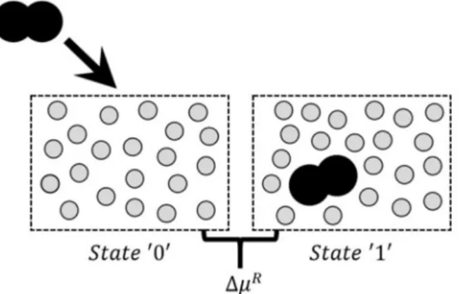
Throughout this work, we use the terms solute and solvent to denote, respectively, the molecule being in-serted and the set of molecules that already exist in the system. This is done even when all molecules are identical. Under these conditions, the residual chemi-cal potential (μR_{) depends only on the probability of a}

successful insertion. This corresponds to the free ener-gy variation of the solvent from the initial state in the

absence of any solute (state ‘0’) to the final state in the

presence of the inserted molecule (state ‘1’), as illus-trated in Figure 1. A hard-sphere solvent and a fused--sphere dimer solute were used as an example. Note that the solute is never really inserted in the simulated system because the successful attempts are recorded, but they are never actually performed.

)

ln(

p

T

k

R

−

=

µ

(1)

Figure 1: Illustration of the Widom method. An example of dimer insertion

in hard-sphere solvent at infinite dilution. The chemical potential depends

As mentioned before, this method is limited to low densities and to molecules with simple structu-res (Labìk et al., 1995; Kofke and Cummings, 1998; Boulougouris et al., 1999; Boulougouris, 2010). At hi-gh densities or for systems with hihi-gher complexity, the

insertion method requires a significant computational effort, that is, a large number of samples is necessary

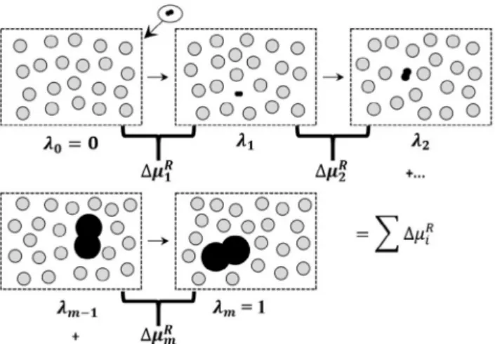
to achieve an adequate statistical sampling. In order to solve this issue, we propose here a stepwise path to the solute insertion.

The proposed path consists in inserting the molecu-le into the solvent in a small scamolecu-le and then increasing it until the inserted solute reaches its real size. The so-lute structure is unaltered, in the sense that all sizes and distances vary proportionally according to a sca-ling factor λ_i ∈[0,1], in which represents a simulation step. For each transition of state from λ_i-1 to λ_i , a Monte Carlo simulation is carried out and the chemical po-tentials for intermediate steps are obtained. Given that thermodynamic properties depend only on the initial

and final states, the total residual chemical potential

will be the sum of all stepwise contributions.

Hereafter, we show that this procedure is thermody-namically consistent. Consider an athermic, N-particle system at constant volume V whose potential energy U consists of two terms as in:

We can obtain Equation (4) for the residual chemi-cal potential by integrating the residual free energy:

∑

∑ ∑

+

=

r

u

j

u

r

r

U

2 2 1

2

1

,

,...,

)

(

1

,

,

)

(

)

(

λ

λ

The second term of Equation (2) represents the interaction of all other particles amongst themselves. Here, we adopted the hard-core potential model.

The first term, presented below, corresponds to the

potential energy of interaction between the molecule to be inserted (1) and all other molecules in the system (j). This term depends on the coupling factor λ such that, for λ = 0, the first term is “decoupled” from the

system, while for λ = 1 the first term corresponds to the potential energy with the molecule completely inser-ted. Between these two values of λ, the potential varies continuously. This dependency is generally linear, but may be non-linear as, for example, for hard-core po-tentials applied here.







=

=

=

1

),

,...,

,

(

0

),

,...,

,

(

)

,

,

1

(

λ

λ

λ

if

r

r

r

u

if

r

r

r

u

j

u

The residual chemical potential can be defined as

a partial derivative of the residual Helmholtz energy (Hill, 1960) as

) 1 , , ( ) , , ( ) 1 ( ) 1 , , ( ) , , ( ) , , ( , − − = − − − − ≅       ∂ ∂ = N V T A N V T A N N N V T A N V T A N A N V T R R R R V T R R µ (4)

λ

λ

λ

µ

µ

d

A

T

k

T

k

T

k

R b b m R b R

∫



_



∂

_∂



_



=

=

0 , ,

1

)

(

(5)

Then, we rearrange to represent all the simulation steps of the proposed algorithm,

λ λ λ λ λ λ µ λ λ λ λ d A T k d A T k d A T k T k N V T R b N V T R b N V T R b b R

m ,, 1 , , , , 0 1 2 1 1 ₁ ... 1 1 ∫ ∫ ∫ −       ∂ ∂ + +       ∂ ∂ +       ∂ ∂ = ₍₆₎

Finally, one can calculate the residual chemical po-tential from:

∑

0 1 1 2 1 1

... λ λ λ

λ λ

λ µ µ µ

µ µ

(7)

The method performs insertion attempts of the solute on its initial scale (λ₁) to obtain the insertion

chemical potential increment (∆μ₁R_{). This procedure}

is identical to the conventional Widom method. The other steps intend to obtain the probabilities of

incre-asing the solute by a pre-determined increment ∆λi of

the scaling factor. Separate simulations carry out each step. This is an advantage because one can perform it in parallel. For these stages, the probability to incre-ase the solute from a state i - 1 to the next state i is obtained by simulating the system with the solute alre-ady inserted with scale λ_i-1. This procedure consists of multiplying the full-size atomic radii and interatomic distances by λ_i = λ_i-1 + ∆λ_i and recording the number of successful attempts. At the end of all simulations, the

residual chemical potential between initial and final

states is given by:

MONTE CARLO SIMULATIONS

The Monte Carlo simulations followed the Metropolis method at constant volume (V) and cons-tant number of molecules (N) for athermic systems. The hard-core potential was applied in all simulated systems to obtain only entropic contributions. Thus, we calculated the free energy taking into account only

the configuration because we used no attractive ener -getic interactions.

The volume of the simulation box was determined from the desired reduced density ρ* = (N_HS/V)σ_s3_,

whe-re σ_s is the diameter of the hard sphere which consti-tutes the solvent molecules, since in this work all the spheres present in the solvent have the same diameter and N_HS is the number of hard-spheres present in the solvent. We used cubic geometry for all simulations boxes. Furthermore, we applied periodic boundary

conditions in all directions. The initial configurations

were generated using the software package Packmol

(Martínez et al., 2009). To reduce computational effort

with the overlap-test procedure, we implemented a nei-ghbor list technique based on that of Yao et al. (2004).

We reproduced each simulation ten times inde-pendently, with the purpose of estimating the residual chemical potential uncertainties. For each stage i, we obtained the average of the probability and its standard deviation (SD). As the chemical potential has the form

) ln( _i

b R

i k T p

f =

µ

Figure 2: Illustrative scheme for the proposed gradual insertion. We

present a dimer insertion in a fluid of hard sphere. Each simulation step

results in a free energy increment. Initially, the residual chemical potential corresponding to the insertion of the small dimer (λ) is calculated. Then, we obtain the residual chemical potential for each step up to the last one,

with the final step λm = 1, which corresponds to the solute molecule at its

real size.

∑

=

−

−

−

=

i

i i b

R

p

p

T

k

, 1

1

)

ln(

)

ln(

µ

(8)

where p₁ is the probability of a successful solute in-sertion attempt from λ₀ = 0 to λ₁ and p_i-1,i is the pro-bability of a successful increase of the solute size from λ_i-1 to λ_i. Even though we have shown Equation (8) for a pure component, the extension to mixtures is straightforward.

2 2

   

  − =

i p

p SD

SD i

i

µ (9)

where SD_pᵢ and SD_μᵢ are the probability and chemical potential standard deviations at the stage i, respectively.

The estimated errors for all stages lead to a

propa-gation of uncertainty at the final chemical potential. The final chemical potential is a linear combination of

the kind

_∑

= m

i m mA

a f

0

, and because the replicas were

in-dependently measured there were no covariance and the combinatorial factor was null. Thus, we can obtain the standard deviation from

∑

=

=

m

i

i

SD SD

0 2 2

µ

µ (10)

where SD_μ is the final chemical potential standard

Here, we define a cycle as a set of operations ran -domly proposed, performed in sequence. At each

cycle, “N” molecules were randomly selected from the

system one at a time. For each random molecule, we proposed a random operation. Because we considered a rigid molecular structure, there were only two pos-sible moves to be performed with the solvent molecu-les: rotation and translation. The translation move was applied to the geometric center, with initial position

r = (r_x,r_y,r_z), according to the procedure described in Allen and Tildesley (1987). The rotation move was applied with a randomly chosen rotation angle

betwe-en -∆θ_max and ∆θ_max about one of the three orthonormal axis (x,y,z) also determined at random. The adopted probability of translation and rotation proposals was 50% for each. We performed these proposals for ran-domly selected molecules from the solvent.

In order to obtain the residual chemical potential,

the first stage of the stepwise path corresponds to the

Widom insertion method. The insertion of the solute molecule was attempted at each 20 cycles with λ₁ = 0.1,

that means 10% of its real scale. The fixed sampling

interval does not obey the detailed balance condition,

but satisfies the weaker balance condition that is consi

-dered mathematically sufficient (Manousiouthakis and

Deem, 1999; Ren et al., 2007; Earl and Deem, 2008; Suwa and Todo, 2010). For the insertion, we selected a uniformly distributed random position and a random orientation. Given the problems of non-uniformity and irreversibility described by Brannon et al. (2002), we applied the quaternion rotation to select a random orientation uniformly for the insertion step. This ap-proach solves rotation problems in an uncomplicated way without the use of coordinates, allowing a more compact representation of the rotation and is free of the singularity problem (Karney, 2007).

To generate a uniform quaternion, the SHOEMAKE algorithm described by Brannon et al. (2002) was used. Then, we applied the quaternion rotation matrix of the SHOEMAKE form to the geometric center of the solu-te structure. With the chosen orientation, we execusolu-ted an attempt to insert the solute in the random position.

In the developed algorithm, the proposed coordinates were accepted or rejected according to an overlap test (Metropolis criterion). Thus, the moves

that resulted in overlaps (∆U = ∞) were rejected. Those

that did not result in overlaps (∆U = 0) were accepted.

We verified the absence of overlaps by calculating the

shortest distance between each atom of the chosen molecule to the other atoms in the system (considering

the minimum image convention).

For the insertion step, the total number of attempted insertions of the small solute molecule (λ₁ = 0.1) and the number of virtually accepted ones were recorded. At the end of a simulation, we used these values to obtain the insertion probability, corresponding to the

first transition, according to Equation (1). The other

simulations were designed to obtain the intermediate probabilities for the gradual increases.

The algorithm implemented for the particle growth was similar to the Widom method. Instead of inserting the solute into the system, the reduced molecule was

already present in the solvent. The main difference lies

in that we replaced the virtual insertion attempt by a virtual increase attempt for the solute. This was done by multiplying the solute structure and diameters by the corresponding scale factor. Therefore, to increase from λ_i-1 to λ_i, we multiplied the real distance of each solute atom from the geometric center of the molecule by the scale factor λ_i. We did the same for the diame-ters. To obtain the increase in probability for each state transition, we used the number of accepted moves and the total number of attempts. For this work, we

adop-ted an increment ∆λ of 0.1. We obtained the chemical potential from Equation (8).

RESULTS AND DISCUSSION

Validation results

Initially, test simulations with the original Widom method (that is, with a single insertion step) were exe-cuted so as to reproduce simulations for highly dilute solutions of spheres in spheres carried out by de Souza et al. (1994), and of dimers in spheres performed by Stamatopoulou et al. ( 1995), respectively. The succes-sful insertion probability and chemical potential were obtained as a function of the diameter ratio, given by:

s

d

σ

σ

1

1

=

where σ₁ is the segment diameter of the solute (the lar-gest one in the case of solutes composed of distinct spheres) and σ_S is the diameter of the solvent.

For sphere-in-sphere solutions, a solvent medium constituted of 108 hard spheres was simulated as in de Souza et al. (1994) for reduced density values of 0.1, 0.4, and 0.8. Each run consisted of 105 _{Monte Carlo}

cycles, from which the first 104 _{cycles were discarded}

simulation results and those from de Souza et al. (1994). The results were also compared with the residual chemical

potential at infinite dilution obtained from the Boublik-Mansoori-Carnahan-Starling-Leland (BMSCL) equation of

state for hard sphere mixtures (de Souza et al., 1994), which is given by:

We performed additional simulations by varying

the density while keeping a fixed diameter ratio of

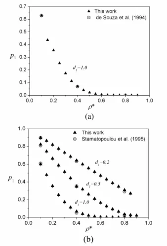
1.0 for hard-sphere systems in order to observe the density-related limitation of the Widom method. We carried out simulations at reduced densities between 0.1 and 0.9. In Figure 5, we show the results in terms of insertion probabilities to highlight the high-density problem. The insertion probabilities, shown in Figure

5a, approach zero as the density increases. This figu

-re illustrates the inc-reasing difficulty of inserting the

solute and, consequently, of obtaining the correct pro-bability if the original Widom method is employed. Quantitatively, the percentage deviation varied from 0.11% at ρ* = 0.1 to almost 60%, at ρ* = 0.9. These values exemplify the large uncertainty in the single--step method for higher density systems, with equal number of cycles. Therefore, we can verify that such a bad sampling takes place even for the simplest

syste-ms. The insertion probability difficulties are going to

be worse for large molecules.

(

)

1

(

2

3

1

)

ln

(

1

)

,

)

1

(

3

)

1

(

3

1

2

2 1 2

2 1 3

3 1 ,

η

η

η

η

η

η

η

µ

−

−

+

−

+

−

−

+

+

−

+

−

=

∞

d

d

d

d

d

d

T

k

R i

(12)

in which η represents the packing fraction, that is,

The single-step insertion of dimers in hard-sphere solvents was simulated and the results were compared to those from Stamatopoulou et al. (1995). In this case, the solute is a diatomic molecule with atomic diameters of 1.75 Å and 1.20 Å, and a bond length of 1.27 Å. The reduced densities of the solvent were 0.1, 0.4, and 0.8. For this system, σ₁ corresponds to the diameter of the largest sphere that composes the dimer, i.e., σ₁ = 1.75 Å. The solvent contained 108 hard-sphere

particles. Again, it can be verified in Figure 4 that a

good agreement occurred between the results obtained in the present work and those from Stamatopoulou et al. (1995).

Figure 3: Residual chemical potential at infinite dilution vs. diameter

ratio for hard sphere-in-sphere mixtures. The simulation results are in good agreement with the de Souza et al. (1994) and BMCSL results. This validates our single-step insertion method for hard sphere systems.

(13)

,

6

*

6

3

πρ

σ

π

η



=























=

V

N

Figure 4: Probability of a successful insertion (p1) vs. diameter ratio (d1)

for dimer-in-sphere mixtures at infinite dilution. The simulation results are

One can verify the same behavior for homonuclear tangent dimers in spheres. We choose three diameter ratios, namely 0.2, 0.5, and 1.0. The reduced density ranged from 0.1 to 0.9. The results, shown in Figure 5b, illustrate a reduction in the probability of insertion with the increase of the system density for all three--diameter ratios. As expected, the lower the diameter ratio the higher is the insertion acceptance frequency for a given density. The percentage deviation for this system varied from 0.06%, at ρ* = 0.1, to 0.9%, at ρ* = 0.85, for d₁ = 0.2. This small variation is related to

the small diameter ratio, which does not present diffi -culties in the insertion process. For d₁ = 0.5, we have deviations of 0.15% at ρ* =0.1 and of 8.37% at ρ* =

0.9. Thus, we observe the insertion difficulty beco -ming problematic for the direct insertion method. The increase of uncertainty with the density increase beco-mes even larger for d₁ = 1.0. In this density, we have

a percentage deviation of 0.15% at ρ* = 0.1 to almost 30% at ρ* = 0.85.

Once we had validated the basic algorithm with one-step movement (insertion), the proposed metho-dology with multiple steps can be tested, as presented hereafter. We validated the proposed stepwise inser-tion Monte Carlo method through the calculainser-tion of residual chemical potentials of highly dilute trimers in spheres. The trimers are composed of identical sphe-res whose centers form an equilateral triangle with side length equal to one spherical diameter, so that we could reproduce the results of Ben-Amotz et al. (1997). The simulation box contained 256 spheres and the diameter ratio d₁ = σ₁/σ_S varied from 0.1 to 0.9 at the reduced densities of 0.1, 0.5, and 0.8.

Results are presented in Figure 6 and were compa-red with those of Ben-Amotz et al. (1997), who

calcu-lated the chemical potential with two different metho -dologies, both based on the Widom insertion method. One can observe an increase of residual chemical po-tential with the increase of the diameter ratio. Again, solutes with smaller diameter ratios require smaller free volume for successful insertions, which then

lo-wer the residual chemical potential. This effect is mo -re important at high densities (liquid phase). From the results, we can only verify that the agreement with the literature and the calculation capacity of our method

were satisfied. To compare the methods we have no

exact information of the chemical potentials and the error values obtained by Ben-Amotz et al (1997).

Figure 5: Probability of successful insertion vs. reduced density (ρ*).

(a) Hard sphere mixtures at infinite dilution. (b) Dimer in hard spheres at high dilution. In both figures, we illustrate the problem of insertion at

high densities: as the reduced density increases, the insertion probabilities approach zero.

Figure 6: Chemical potential of trimers in spheres at infinite dilution vs.

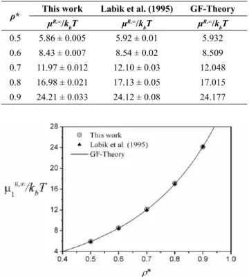
We also applied the proposed method to systems constituted only of dimer molecules. Similar simula-tions were performed by Labìk et al. (1995) for a ho-monuclear, tangent dimer solute at reduced densities of 0.5, 0.6, 0.7, 0.8, and 0.9. They simulated systems with lower diameter solute and extrapolated the results to obtain the chemical potentials for higher diameters. We carried out all simulations with 600 solvent parti-cles for this system. The results presented in Table 1 and Figure 7 show good agreement with those from Labìk et al. (1995) for "n = 3" (polynomial order of the extrapolation equation), considered by the authors as their more accurate results. Table 1 and Figure 7 also contain calculated residual chemical potentials from the Generalized Flory–(r’-mer) Theory (GF-Theory) (Escobedo and de Pablo, 1995; Honnell and Hall, 1989) equation of state, which are also close to

our values. In addition, it can be verified that the calcu -lated errors were smaller than those from Labìk et al. (1995), showing that the use of the proposed methodo-logy can obtain reliable values for chemical potentials with lower uncertainty.

Sphere + dimer mixtures

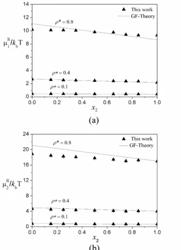
We applied the proposed methodology to mixtures of hard spheres (1) and dimers (2) of varying

concen-trations and at reduced density of mixture (defined as

(

)

(

)

2 3

1 2

1 2

* σ σ

ρ = NHS V + NHS V , in which σ₁ = σ₂ of 0.1,

0.4, and 0.8. For all simulations, the adopted

incre-ment for the scale factor was ∆λ = 0.1. At each density,

sphere+dimer mixtures with different concentrations

were considered as the solvent, while either a dimer or a hard sphere was considered as the solute. Each run contained 107 _{cycles, from which the 500000}

ini-tial ones were discarded, and 475000 transitions were attempted in each stage of solute growth. We tested si-mulation boxes with 300, 500, 800, and 1200 particles

to check for finite-size effects. The chosen number of

particles was equal to 800 for ρ* = 0.8 and 300 for lo-wer densities (0.4 and 0.1). Note that all dimers simu-lated in this mixture were homonuclear and tangent, and we assumed the diameter ratio to be unitary.

We present the obtained residual chemical potentials in Figure 8a for hard spheres and in Figure 8b for dimers. The results were compared with predictions of the GF-Theory as presented by Escobedo and de Pablo (1995). For pure systems, the chemical potential of each component (μᵢR,ͦ_{) was obtained from the}

integration of the equation of state, expressed in terms of compressibility factor (Z) of hard chains as:

Table 1. Residual chemical potential for homonucle-ar, tangent dimer system.

ρ* This work Labìk et al. (1995) GF-Theory μR,∞_/k

bT μ

R,∞_/k

bT μ

R,∞_/k bT 0.5 5.86 ± 0.005 5.92 ± 0.01 5.932

0.6 8.43 ± 0.007 8.54 ± 0.02 8.509

0.7 11.97 ± 0.012 12.10 ± 0.03 12.048

0.8 16.98 ± 0.021 17.13 ± 0.05 17.015

0.9 24.21 ± 0.033 24.12 ± 0.08 24.177

Figure 7: Chemical potential of dimers in dimers at infinite dilution

vs. reduced density. The calculated residual chemical potentials were consistent with those from Labìk et al. (1995) and the GF-Theory model. As expected, we observe an increase of chemical potential as the density increases.

.

)

1

(

1

3 3 3 2 2 1

η

η

η

η

−

+

+

+

=

c

c

c

Z

The constants used for the equation of state model were taken from Escobedo and de Pablo (1995). For a sphere (monomer), they are c₁ = 1.0, c₂ = 1.0, and

c₃ = -1.0, while for dimers they are c₁ = 2.45696, c₂ = 4.10386, and c₃ = -3.75503.

For binary mixtures, an analogy to GF-Theory (Honnell and Hall, 1989; Escobedo and de Pablo, 1995) proposed by Honnell et al. (1989) was applied as a free volume correction. For a two-component sys-tem, we applied the analogy as:

,

2 , 1 , 1

,

x

v

v

v

Y

L L L n

−

=

,

2 , 1 , 2

,

x

v

v

v

Y

L L L n

−

where Y_n corresponds to a correction term based on

free volume differences between dimer and monomer

systems, representing the free volume change with the presence of other components. The term V_L,1 is the free volume of a system constituted only of monomers and the term V_L,2 is the free volume of a system constitu-ted only of dimers. The values used were V_L,1 =4/3 and

V_L,2 = 9/4 (Escobedo and de Pablo, 1995).

When x₁ →0 we have that Y_n,2 → 0 , and the

residual chemical potentials turn into μ₂R,ͦ _{(pure) and}

μ₁R,∞(infinite dilution). In addition, when _x

1 → 1, Y_n,2 becomes the correction for the case in which all solvent particles are replaced by hard-spheres and we have μ₁R,ͦ and μ

2

R,∞_.

In Figure 8 one can observe good agreement be-tween simulation results and equation-of-state calcula-tions regarding residual chemical potentials of

compo-nents 1 and 2 at mixtures with different compositions,

especially at the lowest densities. As expected, the equation of state presented larger deviations at the hi-ghest density, ρ* = 0.8. However, the results followed a similar trend.

In Figure 8 the residual chemical potentials of both spheres and dimers decrease with increasing concen-tration of dimers. We expected this behavior because the arrangement of dimer molecules results in a greater volume of interstices due to their geometric constraint. Thus, a higher concentration of dimer molecules makes it easier to insert the solute and, consequently, lowers the residual chemical potential. Although we have

si-mulated different size boxes, the percentage deviations presented a small variation between the different den -sities, compared with the single-step method. For the hard-sphere residual chemical potential, the percenta-ge deviation was in the ranpercenta-ge of 0.083 to 0.177%. For the dimer residual chemical potential, that range was from 0.02 to 0.20%.

To study the effect of free volume, we calculated the residual chemical potential of dimers with diffe -rent ratios of bond length/sphere diameter (l/σ₁) at

infinite dilution having hard spheres as solvents. In

Figure 9, the l/σ ratio variation for homonuclear dimer

particles is illustrated. Observe that, when l/σ is zero, the dimer is reduced to a sphere, thus identical to the solvent molecules. At the other extreme (l/σ = 1), the dimer becomes a pair of tangent spheres.

In Figure 10, at low densities, there is almost no

di-fference among the curves. This can be assigned to the

largely similar solute structures and a larger interstitial

space present at low densities. Nonetheless, the diffe -rence increases as the reduced density also increases. At high densities, the interstitial space becomes incre-asingly restricted and, accordingly, the bond length becomes an important factor for the insertion probabi-lity. For higher l/σ ratio values, the residual chemical

potential increases. Thus, a dimer with greater bond

length is more difficult to insert. We observe a linear

(

)

2 1 , , 1 1 , ,

1

1

R n R n

R

mix

Y

µ

Y

µ

µ

=

+

+

(

)

1 1 , , 2 2 , ,

2

1

R n R n

R

mix

Y

µ

Y

µ

µ

=

+

+

Figure 8: Residual chemical potential of solute vs. dimer fraction in the solvent, at the reduced densities of 0.1, 0.4 and 0.8. (a) Sphere as solute. (b) Dimer as solute. The residual chemical potential decreases with increasing concentration of dimers for both solutes. This behavior is consistent with the fact that a dimer molecule contains a greater volume of void space.

relationship between the chemical potential and the l/σ ratio at all studied densities. The curve slope increa-ses with increasing density, from 0.2334 at ρ* = 0.1 to 8.3414 at ρ* = 0.8. This quantifies the great influence

of density in calculating the chemical potential in a way that makes other factors such as the bond length

more influential.

CONCLUSIONS

The application of the Widom insertion method is a traditional way to obtain chemical potentials. However, it is limited to simple and low-density syste-ms because its computational demand tends to become impracticable for complex molecules, especially at hi-gh densities. Based on the Widom method, we propo-sed an intermediate path to obtain chemical potentials of rigid molecules with hard-core potential in order to overcome the Widom method’s limitation.

We validated the implemented Monte Carlo algo-rithm by comparing results obtained by the Widom

method for sphere and dimer solutes infinitely diluted in sphere solvents. We verified the proposed metho -dology by comparing simulations of trimers in sphe-res and dimers in dimers with sphe-results from the litera-ture. The proposed method generated similar results with lower uncertainties, especially at high densities. Then, we applied the method to systems constituted of hard-spheres and dimers. We analyzed the behavior of chemical potentials with dimer concentration to in-vestigate the potential use of the proposed method in thermodynamics studies. The calculated residual che-mical potential of each component decreases as the dimer concentration becomes higher. It corresponds

Figure 10: Residual chemical potential of dimers at infinite dilution vs. l/σ

ratio, for different reduced densities ρ*. The influence of l/σ on the residual chemical is linear in all densities studied.

to the expected behavior because dimers systems pre-sent more free space. In turn, the obtained uncertainty is promising for the obtainment of entropic residual chemical potentials even at higher densities, allowing its use in systems in the liquid state. We also obtained

the residual chemical potential at infinite dilution of

a dimer in hard spheres varying its bond length. We

observed that the bond length had a higher influence in

higher density systems.

In general, the methodology of gradual solute

inser-tion was effective for both low and high densities for

all systems studied. The calculated residual chemical potentials were consistent with the expected results. Future work will explore the range of applicability of this method to systems with increased complexity such as hard chain and real systems. In addition, the study of the applied λ increment is necessary.

REFERENCES

Allen, M. P. and Tildesley, D. J., Computer simulation of liquids. Oxford Press, Oxford (1987).

Ben-Amotz, D., Stamatopoulou, A. and Yoon, B.J., Three-body distribution functions in hard sphere

fluids. Comparison of excluded- volume-anisotropy

model predictions and Monte Carlo simulation. The Journal of Chemical Physics, 107, 6831–6838 (1997).

Boulougouris, G. C., Calculation of the Chemical Potential beyond the First-Order Free-Energy Perturbation: From Deletion to Reinsertion. Journal of Chemical and Engineering Data, 55, 4140–4146 (2010).

Boulougouris, G. C., Economou, I. G. and Theodorou, D. N., On the calculation of the chemical potential using the particle deletion scheme. Molecular Physics, 96, 905–913, (1999).

Brannon, R. M., A review of useful theorems involving proper orthogonal matrices referenced to three-dimensional physical space. Albuquerque, Sandia National Laboratories (2002). Available from: <http://www.mech.utah.edu/~brannon/public/ rotation.pdf>

De Souza, L. E. S., Stamatopoulou, A. and Ben-Amotz, D., Chemical potentials of hard sphere solutes in hard sphere solvents. Monte Carlo simulations and analytical approximations. The Journal of Chemical Physics, 100, 1456–1459 (1994).

Dietrick, G. L., Scriven, L. E. and Davis, H. T.,

Efficient molecular simulation of chemical

Earl, D. J. and Deem, M. W., Parallel Tempering : Theory , Applications , and New Perspectives. 1–21 (2008).

Escobedo, F. A. and De pablo, J. J., Chemical potential and equations of state of hard core chain molecules. The Journal of Chemical Physics, 103, 1946–1956, (1995a).

Escobedo, F. A. and De pablo, J. J,. Monte Carlo simulation of the chemical potential of polymers in an expanded ensemble. The Journal of Chemical Physics, 103, 2703–2710, (1995b).

Fay, P. J., Ray, J. R. and Wolf, R. J., Detailed balance methods for chemical potential determination. The Journal of Chemical Physics, 103, 7556, (1995). FrenkeL, D. and Smit, B., Understanding molecular

simulation From algorithms to applications. New York, Academic Press (1996).

Hill, T. L., An introduction to Statistical Thermodynamics. New York: Dover Publications, 1960.

Honnell, K. G. and Hall, C. K. A, new equation of state for athermal chains. The Journal of Chemical Physics, 90, 1841 (1989).

Karney, C. F. F., Quaternions in molecular modeling. 25, 595–604 (2007).

Koda, T. and Ikeda, S., Test of the scaled particle theory for aligned hard spherocylinders using Monte Carlo simulation. The Journal of Chemical Physics, 116, 5825 (2002).

Kofke, D. A. and Cummings, P. T. Precision and accuracy of staged free-energy perturbation methods for computing the chemical potential by molecular simulation. Fluid Phase Equilibria, 150-151, 41–49, (1998).

Kristóf, T. and Rutkai, G., Chemical potential calculations by thermodynamic integration with separation shifting in adaptive sampling Monte Carlo simulations. Chemical Physics Letters, 445, 74–78 (2007).

Labìk, S., Jirásek, V., Malijevský, A. and Smith, W.

R. , Modifications of the SP-MC method for the

computer simulation of chemical potentials: ternary

mixtures of fused hard sphere fluids. Molecular

Physics, 94:2, 385–393 (1998).

Labìk, S. Jirásek, V., Malijevský, A. and Smith, W. R., Computer simulation of the chemical potentials

of fused hard sphere diatomic fluids. Chemical

Physics Letters, 247, 227–231 (1995).

Labík, S. and Smith, W. R., Scaled Particle Theory and

the Efficient Calculation of the Chemical Potential

of Hard Spheres in the NVT Ensemble. Molecular Simulation, 12:1, 23–31, (1994).

Manousiouthakis, V. I. and Deem, M. W., Strict detailed balance is unnecessary in Monte Carlo simulation. The Journal of Chemical Physics, 110, 2753 (1999).

Martínez, L., Andrade, R., Brigin, E. G., Martínez J. M., PACKMOL: A Package for Building

Initial Configurations for Molecular Dynamics

Simulations. Journal of Computational Chemistry, 30, 2157–2164 (2009).

Mehrotra, A. S., PurI, S. and Khakhar, D. V., Field induced gradient simulations: A high throughput method for computing chemical potentials in multicomponent systems. The Journal of Chemical Physics, 136, 134108 (2012).

Mon, K. K. and Griffiths, R. B., Chemical potential

by gradual insertion of a particle in Monte Carlo simulation. Physical Review A, 31, 956–959 (1985).

Ren, R., O’Keeffe, C. J. and Orkoulas, G., Sequential metropolis algorithms for fluid simulations.

International Journal of Thermophysics, 28, 520– 535 (2007).

Stamatopoulou, A., de Souza, L. E. S., Bem-Amotz, D. and Talbot, J., Chemical potentials of hard

molecular solutes in hard sphere fluids. Monte

Carlo stimulations and analytical approximations. The Journal of Chemical Physics, 102, 2109–2112 (1995).

Suwa, H. and Todo, S., Markov Chain Monte Carlo Method without Detailed Balance. Phys. Rev. Lett., 1–5 (2010).

Tej, M. K. and Meredith, J. C., Simulation of nanocolloid chemical potentials in a hard-sphere polymer solution: Expanded ensemble Monte Carlo. The Journal of Chemical Physics, 117, 5443 (2002).

Torrie, G. M. and Valleau, J. P., Nonphysical Sampling Distributions in Monte Carlo Free-energy Estimation: Umbrella Sampling. Journal of Computational Physics, 23, 187–199 (1977). Virnau, P. and Müller, M., Calculation of free energy

through sucessive umbrella sampling. Journal of Chemical Physics, 120, 10925 (2004).

Widom, B. Some Topics in the Theory of Fluid. Journal of Chemical Physics, 39, 2808–28012, (1963).