Licenciado em Ciências da Engenharia Electrotécnica e de Computadores
Context-based Identification of Energy
Consumption in Industrial Plants
Dissertação para obtenção do Grau de Mestre em Engenharia Electrotécnica e de Computadores
Orientador :
Prof. Doutor Rui Neves-Silva, Professor Auxiliar,
Universidade Nova de Lisboa
Júri:
Presidente: Prof. Doutor Paulo José Carrilho de Sousa Gil
Arguente: Prof. Doutora Maria Júlia Fonseca de Seixas
Graduated Studies in Electrical and Computer Engineering
Context-based Identification of Energy
Consumption in Industrial Plants
Dissertation to obtain the Master Degree in Electrical and Computer Engineering
Supervisor:
Prof. Rui Neves-Silva, PhD, Assistant Professor,
Universidade Nova de Lisboa
Evaluation Board:
President: Prof. Paulo José Carrilho de Sousa Gil, PhD
Opponent: Prof. Maria Júlia Fonseca de Seixas, PhD
Copyright cJoão Manuel da Costa e Cruz, Faculdade de Ciências e Tecnologia,
Univer-sidade Nova de Lisboa
A Faculdade de Ciências e Tecnologia e a Universidade Nova de Lisboa têm o direito, perpétuo e sem limites geográficos, de arquivar e publicar esta dissertação através de exemplares impressos re-produzidos em papel ou de forma digital, ou por qualquer outro meio conhecido ou que venha a ser inventado, e de a divulgar através de repositórios científicos e de admitir a sua cópia e distribuição com objectivos educacionais ou de investigação, não comerciais, desde que seja dado crédito ao autor e editor.
Acknowledgements
I take this space to leave my sincere thanks to all who contributed to the accomplish-ment of this work.
To Professor Rui Neves-Silva, who I greatly admire, for his availability, guidance and support through all the stages of this work.
To my Professors Luís Brito Palma and Fernando Coito, from who I learned a lot, for all the knowledge shared.
To my colleagues, André Águas, Daniel Marques, Ricardo Mota and Sérgio Coelho for their continuous motivation, but most of all, for their friendship and all the moments we shared together
To Eng. Tiago Gonçalves, CEO of InnoWave Technologies, for his understanding and motivation given during the last stage of my dissertation
To my family from who I’m eternally grateful, who always give me support and hap-piness. I also take this opportunity to express my sincere apologies, for all the time I was absent.
upon the shoulders of giants.”
Abstract
Nowadays, reducing energy consumption is one of the highest priorities and biggest challenges faced worldwide and in particular in the industrial sector. Given the increas-ing trend of consumption and the current economical crisis, identifyincreas-ing cost reductions on the most energy-intensive sectors has become one of the main concerns among com-panies and researchers.
Particularly in industrial environments, energy consumption is affected by several factors, namely production factors(e.g. equipments), human (e.g. operators experience), environmental (e.g. temperature), among others, which influence the way of how en-ergy is used across the plant. Therefore, several approaches for identifying consumption causes have been suggested and discussed. However, the existing methods only provide guidelines for energy consumption and have shown difficulties in explaining certain en-ergy consumption patterns due to the lack of structure to incorporate context influence, hence are not able to track down the causes of consumption to a process level, where optimization measures can actually take place.
This dissertation proposes a new approach to tackle this issue, by on-line estimation of context-based energy consumption models, which are able to map operating context to consumption patterns. Context identification is performed by regression tree algorithms. Energy consumption estimation is achieved by means of a multi-model architecture using multiple RLS algorithms, locally estimated for each operating context.
Lastly, the proposed approach is applied to a real cement plant grinding circuit. Ex-perimental results prove the viability of the overall system, regarding both automatic context identification and energy consumption estimation.
Keywords: Energy consumption; Context awareness; Regression tree; Multi-models;
Resumo
Atualmente, um dos grandes desafios a nível mundial e em particular no setor indus-trial, é reduzir o consumo energético. Dada a atual crise económica e o contínuo aumento do consumo, a identificação de possíveis situações de redução de custo tem-se tornado uma das principais preocupações entre empresas e investigadores.
Em meio industrial, o consumo energético é afetado por vários fatores, nomeada-mente fatores de produção (e.g. equipamentos), humanos (e.g. experiência do operador), ambientais (e.g. temperatura), entre outros, que influenciam a forma como a energia é usada pela instalação. Com o objetivo de identificar como estes fatores influenciam o consumo, várias metodologias têm sido sugeridas. No entanto, estas apenas fornecem diretrizes, e têm demonstrado dificuldade em explicar determinados padrões de con-sumo devido a não incorporarem uma estrutura que inclua a influência do contexto. Por este motivo, estas técnicas não são capazes rastrear as causas do consumo energético até ao nível do processo, onde efetivamente medidas de otimização podem ser tomadas.
Esta dissertação propõe uma nova abordagem para superar este problema, utilizando modelos de consumo energético baseados em contexto, que relacionam o contexto de operação com os padrões de consumo energético. A identificação de contexto é efetuada através de algoritmos de árvores de regressão e o consumo é estimado através de uma arquitetura baseada em múltiplos modelos locais, por meio de múltiplos algoritmos RLS, um por cada contexto de operação.
Por último, a abordagem proposta é aplicada a um circuito de moagem de cimento. Os resultados experimentais comprovam que a metodologia desenvolvida é viável, tanto na identificação automática de contextos como na estimação do consumo energético.
Palavras-chave: Consumo Energético; Identificação de Contexto; Árvores de regressão;
Contents
1 Introduction 1
1.1 Context and Motivation . . . 1
1.2 Objectives and Original Contributions . . . 2
1.3 Dissertation Organization . . . 2
2 State of Art 5 2.1 Energy Consumption in Industrial Plants . . . 5
2.1.1 Global Energy Use Perspective . . . 5
2.1.2 Energy Consumption Optimization . . . 8
2.1.3 Keeping Track of Energy Consumption . . . 9
2.1.4 Causes and Influences on Energy Consumption . . . 11
2.2 Energy Consumption Models . . . 12
2.2.1 Time-Series Regression Models . . . 13
2.2.2 Artificial Intelligence Models . . . 14
2.3 Summary . . . 17
2.4 Proposed Approach . . . 19
3 Context Identification 21 3.1 Modelling Context Influence . . . 21
3.1.1 Context Variables . . . 21
3.1.2 Operating Context, Regions and Centroids . . . 24
3.1.3 Simulation Example . . . 25
3.2 Automatic Context Identification . . . 26
3.2.1 Regression Tree Algorithm . . . 26
3.2.2 Simulation Example . . . 29
3.3 Multiple Context Variables . . . 31
4.1 Context-based Multi-model Approach . . . 37
4.2 Local Model Estimation . . . 40
4.2.1 Recursive Least Squares Algorithm . . . 40
4.2.2 Simulation Example . . . 41
4.3 Context-Based Multi-model Estimation . . . 43
4.3.1 Bank of Models . . . 43
4.3.2 Model Selection . . . 44
4.3.3 Model Commutation . . . 45
4.3.4 Simulation Example . . . 46
4.3.5 Comparison with Traditional Approach . . . 50
5 Implementation 53 5.1 Developed System . . . 53
5.1.1 Methodology . . . 53
5.1.2 Architecture . . . 54
5.1.3 Functional Steps . . . 55
5.2 Context-Based Identification Simulator . . . 57
5.2.1 Global Overview . . . 57
5.2.2 Block A - Simulation and Experiment Specifications . . . 58
5.2.3 Block B - Context-based Multi-Model Identification Specifications . 60 5.2.4 Block C - Graphical Results . . . 62
5.2.5 Block D - Numerical Results . . . 63
5.2.6 Block E - Menu and Toolbar . . . 65
6 Experimental Results 69 6.1 Cement Manufacturing Process and Grinding Circuit . . . 69
6.2 Cement Mill Data . . . 71
6.3 Context-based Energy Models Results . . . 77
6.3.1 CBEM Initialization . . . 77
6.3.2 CBEM Results of September 2012 . . . 78
6.3.3 CBEM Results of October 2012 . . . 81
6.3.4 CBEM Results of January 2013 . . . 84
6.4 Results Summary and Discussion . . . 86
7 Conclusion and Future Work 89 7.1 Conclusion . . . 89
7.2 Future Work . . . 91
List of Figures
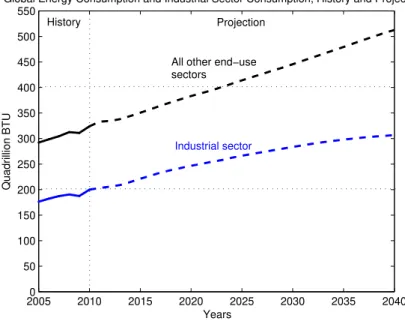
2.1 Global industrial sector and all other end-use energy consumption sectors from 2005 to 2040. . . 6 2.2 Shares of total industrial sector, by the major energy-intensive sectors in
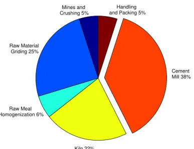
2010. . . 6 2.3 Cement plant energy consumption, divided by the energy-consuming
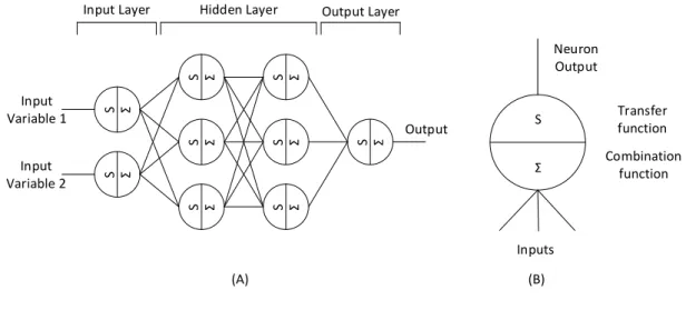
pro-cesses. . . 7 2.4 Basic energy consumption optimization process. . . 8 2.5 Energy track in industrial environments. . . 10 2.6 (A) FFANN configured with 1 input layer, 2 hidden layers and 1 output
layer. (B) Neuron architecture. . . 16
3.1 Representation of a plant from an energy consumption point of view. . . 22 3.2 Representation of a plant from an energy consumption point of view,
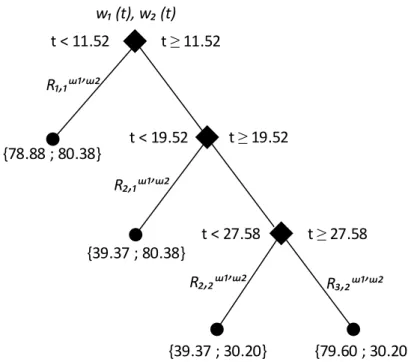
un-der the influence of context. . . 23 3.3 Context influence on energy consumption. The case of a milling unit. . . . 25 3.4 Partition criterion of a regionRrintoRmandRn. . . 28 3.5 Context variable, centroid calculation and region boundaries delimitation 30 3.6 Tree diagram of the LSRT applied tow. . . 30 3.7 Context variablew1 andw2, regions identification and centroid calculation 33
3.8 Tree representation for context variablew1andw2. . . 33
3.9 Context variables overlapped and region intersections. . . 34 3.10 Tree diagram of multiple context variables overlapped and region
inter-sections. . . 35
(C)β = 1(D)β = 5. . . 45 4.6 (A) Plant’s production data. (B) Energy consumption data. (C) Context
variable, regions and centroids. . . 46 4.7 (A) Active model and validity limits. (B) Estimated parameters. . . 48 4.8 Parameter estimation for the upper half and lower half of the context
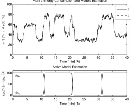
vari-able. . . 48 4.9 (A) Plant energy consumption and CBEM estimation. (B) Local models
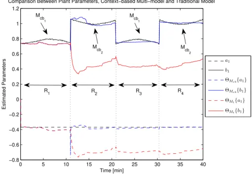
commutation. . . 49 4.10 Comparison between CBEM parameter estimation, tradition approach
es-timation and plant parameter. . . 51 4.11 (A) Comparison between plant energy consumption, CBEM and
tradi-tional approach estimation. (B) Estimation error for both approaches. . . . 52
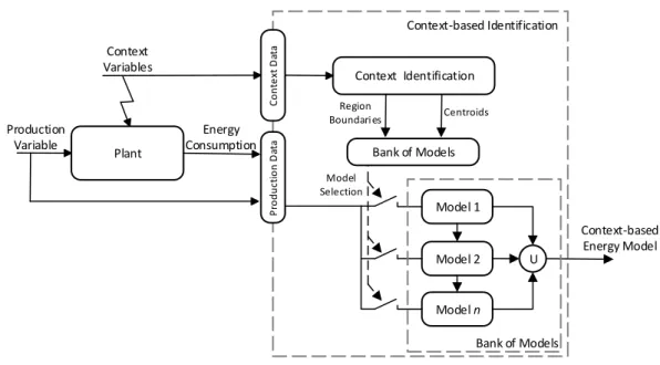
5.1 Schematic illustration of context-based identification stages. . . 54 5.2 Proposed architecture for the context-based energy consumption
identifi-cation system. . . 55 5.3 Functional diagram of the context-based energy consumption system. . . 56 5.4 Context-based energy consumption simulator interface. . . 57 5.5 Simulator interface zoomed on the block A region. . . 58 5.6 Use case UML diagram for (A) simulation and (B) experiment mode. . . . 60 5.7 Simulator interface zoomed on the block B region. . . 60 5.8 Use case UML diagram for context-based mode multi-model identification
specifications. . . 61 5.9 Simulator interface zoomed on the block C region. . . 62 5.10 Use case UML diagram for graphical results. . . 63 5.11 Simulator interface zoomed on the block D region. . . 64 5.12 Use case UML diagram for numerical results. . . 65 5.13 (A) Menu bar and toolbar. (B) File menu options. . . 65 5.14 RLS algorithm specifications. . . 66 5.15 Regression tree viewer. . . 67 5.16 Use case UML diagrams. (A) Application-specific tools. (B) RLS algorithm
specifications and regression tree. . . 67
6.1 Typical cement plant manufacturing process. . . 70 6.2 Cement grinding circuit structure. . . 70 6.3 September 2012 raw data. (A) Flow of input and output materials. (B)
Power consumption. . . 71 6.4 October 2012 raw data. (A) Flow of input and output materials. (B) Power
consumption. . . 73 6.6 September 2012 - Cement specific consumption and cement type. (A)
Spe-cific consumption. (B) Cement type. . . 74 6.7 October 2012 - Cement specific consumption and cement type. (A) Specific
consumption. (B) Cement type. . . 75 6.8 January 2013 - Cement specific consumption and cement type. (A) Specific
consumption. (B) Type of cement. . . 76 6.9 CBEM representation of the milling unit. . . 77 6.10 CBEM context identification results of September 2012 - (A) Type of cement
and centroids zoom on the full month. (B) Active model. . . 78 6.11 CBEM context identification results of September 2012 - (A) Type of cement
and centroids zoom on first cement type A production. (B) Active model. 79 6.12 CBEM prediction results of September 2012 - (A) Specific consumption
prediction. (B) Estimated Parameters. (C) Prediction over a day of operation. 80 6.13 CBEM context identification results of October 2012 - (A) Type of cement
and centroids. (B) Active model. . . 81 6.14 CBEM prediction results of October 2012 - (A) Specific consumption
pre-diction (B) Estimated Parameters. . . 82 6.15 CBEM prediction results of October 2012 zoom on context commutation
-(A) Specific consumption prediction (B) Active model. . . 83 6.16 CBEM context identification results of January 2013 - (A) Type of cement
and centroids. (B) Active model. . . 84 6.17 CBEM prediction results of January 2013 - (A) Specific consumption
pre-diction. (B) Estimated Parameters. (C) Zoom on a type C operating regime. 85
7.1 Future work path: Context-based consumption analysis systems. . . 91 7.2 Future work path: Context-based consumption analysis results. . . 92
A.1 November 2012 raw data. (A) Flow of input and output materials. (B) Power consumption. . . 101 A.2 November 2012 - Cement specific consumption and cement type. (A)
Spe-cific consumption. (B) Type of cement. . . 102 A.3 December 2012 raw data. (A) Flow of input and output materials. (B)
Power consumption. . . 103 A.4 December 2012 - Cement specific consumption and cement type. (A)
Spe-cific consumption. (B) Type of cement. . . 103 A.5 CBEM context identification results of November 2012 - (A) Type of cement
and centroids. (B) Active model. . . 104 A.6 CBEM prediction results of November 2012 - (A) Specific consumption
and centroids. (B) Active model. . . 106 A.8 CBEM prediction results of December 2012 - (A) Specific consumption
List of Tables
3.1 Regions, Centroids and Region Boundaries results. . . 31 3.2 Regions, Centroids and Region Boundaries forw1. . . 34
3.3 Regions, Centroids and Region Boundaries forw2. . . 34
3.4 Regions and Centroids intersection. . . 35
4.1 Estimated Vector of Parameters and Average Absolute Estimation Error . 43 4.2 Regions, Centroids and Region Boundaries. . . 47 4.3 Models, respective centroids and estimated parameters. . . 50 4.4 Comparison between traditional and context-based average absolute
esti-mation error. . . 52
6.1 Data Summary for the months of September, October and January. . . 76 6.2 CBEM system initialization values. . . 78 6.3 Models Estimated in September 2012. . . 80 6.4 CBEM average absolute estimation error for September 2012. . . 80 6.5 Models Estimated in October 2012. . . 83 6.6 CBEM average absolute estimation error for October 2012. . . 83 6.7 Models Estimated in January 2013. . . 85 6.8 CBEM average absolute estimation error for January 2013. . . 85 6.9 Bank of models after 5 months operation. . . 86 6.10 Summary of estimation results. . . 86
List of Symbols
y Energy Consumption.
u Production Variable.
f Mapping Function.
e Disturbances.
w Context Variable.
R Context Region.
c Centroid.
ξ Partition Error.
τ Minimum Period of Steadiness.
κ Quadratic Error Tolerance.
ε Quadratic Error Threshold.
ˆ
f Mapping Function Approximation.
Θ Estimated Vector of Parameters.
tk Discrete Time.
Ts Sampling Period.
ϕ Regression Vector.
ˆ
y Energy Consumption Estimation.
ǫ Estimation Error.
ˆ
ˆ
yM Local Energy Consumption Estimation.
J Cost Function.
PM Local Model Covariance Matrix.
λ Forgetting Factor.
Nλ Forgetting Window.
|∆ǫ| Average Absolute Estimation Error.
N Vector Length.
γ Bank Sensitivity.
Fc Flow of Clinker.
Fg Flow of Gypsum.
Fl Flow of Lime.
Ft Flow of Trass.
Fce Flow of Cement.
Pdrive Drive Power.
ysc Specific Consumption.
Q Ratio of Clinker.
Ftotal Total Flow.
ˆ
Acronyms
FFANN Feed-forward Artificial Neural Network.
LSRT Least Squares Regression Tree.
CBEM Context-based Energy Models.
RLS Recursive Least Squares.
EIA U.S. Energy Information Administration.
SEC Specific Consumption.
EUP Energy Use Parameters.
AI Artificial Intelligence.
SVM Support Vector Machines.
L SVM Linear Support Vector Machines.
NL SVM Non-Linear Support Vector Machines.
LL SVM Locally Linear Support Vector Machines.
LNL SVM Locally Non-Linear Support Vector Machines.
ANN Artificial Neural Network.
GA Genetic Algorithm.
FS Fuzzy Systems.
RT Regression Tree.
1
Introduction
1.1
Context and Motivation
In recent years, competition in the industrial world has become more intense. As a result, the necessity for finding new ways or optimizing energy consumption has in-creased.
To facilitate better planning, companies often maintain databases that store energy consumption measurements along with usage patterns and production data of their ma-jor appliances. These databases are then used to build energy consumption models which help the estimation of energy demand and the identification of possible costs reductions. However, this conventional models, have shown difficulties in explaining certain en-ergy consumption patterns, mostly due to the fact that enen-ergy consumption in industrial plants depend on multiple factors, namely, production factors (e.g. production rates, type of product), human factors (e.g. operator experience), ambient factors (e.g. temperature), among others, and the sum of all of these factors affect the way of how energy is used.
Another driving factor is the recent rapid development of new technologies, which allow the acquisition of information from new sources. Particularly, dispersed contextual information can be acquired by means of dispersed intelligent sensor technology - Am-bient Intelligence (AmI). These new technologies provide the ability of measuring dis-persed contextual information besides the conventional production data, allowing com-panies to build energy consumption models based simultaneously on contextual and production information.
The rise of these new technologies along with the combination of what they provide, will bring companies new opportunities for optimization consumption, driving this work to the study of a method to develop context-based energy consumption models.
1.2
Objectives and Original Contributions
The overall objective of this dissertation is to develop a method to support companies in optimizing their operations and energy savings, by being able to identify how energy is used and employed across the several stages that comprise the company’s production chain.
When process data retrieved from production unit operations is put together with en-ergy consumption information and contextualized into operating contexts, a better un-derstanding of how energy flows through the several production lines is achieved. This work, proposes a new generic and adaptive method for learning energy consumption patterns observed through the production stages, based on the contextual conditions in which production units are operating.
Identifying context-based energy models brings two significant contributions. The first and most evident, is that more accurate estimations of energy consumption can be performed.
The second is the better understanding of how context differently impacts energy consumption, helping companies on finding alternative production strategies.
Both, significantly contribute to better ways of using energy, reducing not only costs but also improving companies overall efficiency.
1.3
Dissertation Organization
This dissertation is organized on 7 chapters (including this one) and 3 appendixes. The rest is organized as follows:
• Chapter 2 - State of Art— It is approached the thematic of energy consumption in
industrial plants, optimization methods and some related works. State of the art consumption models and major applications are also analysed.
• Chapter 3 - Context Identification — It is presented the concept of context
vari-able and how it impacts energy consumption. A regression tree algorithm is pro-posed for context identification followed by computational simulations for theoret-ical demonstration and also for real case scenario framework.
• Chapter 4 - Context-based Energy Models— Is presented the concept of
• Chapter 5 - Implementation — It is depicted the context identification method
incorporated in the multi-model structure and how they play together to build the overall context-based energy models. The description of a simulator developed for demonstration purposes and real case scenarios is also described.
• Chapter 6 - Experimental Results— It is analysed the results of the application
in a real case of a cement plant manufacturing process, focused on the cement mill energy consumption, comprising plant acquired data analysis and results of the developed system. As the experiment was performed for a 5 month mill operation, only 3 months (September 2012, October 2012 and January 2013) with the most relevant data are described in detail. The other 2 months (November and December 2012) are briefly described in Appendix A.1 and A.2.
• Chapter 7 - Conclusion— The main conclusions taken from the developed system
analysis are highlighted and further work paths are suggested.
• Appendix A.1 - Cement Mill Data of November and December 2012— It is
de-picted the acquired data and a brief analysis for the months of November and De-cember 2012.
• Appendix A.2 - CBEM Experimental Results of November and December 2012
— The performance of the developed system is briefly analysed for the months of November and December 2012.
• Appendix A.3 - Publish Paper— Attached the published article resultant from
2
State of Art
In this chapter is performed a brief overview of energy consumption in the industrial sector, starting from current global energy use, narrowing down to the more intensive-energy industrial sectors and main production units.
A top-down approach to keep track of how energy is used across an entire factory is present, along with current methods for optimizing consumption.
Current energy modelling technologies are also described, highlighting its applica-tions, advantages and disadvantages.
Lastly a brief description of this work approach is given, and how it contributes to the overall energy consumption optimization process.
2.1
Energy Consumption in Industrial Plants
2.1.1 Global Energy Use Perspective
According to the U.S. Energy Information Administration (EIA), the industrial sector consumes about 50% of the world’s total delivered energy [1]. (Figure 2.1).
The industrial sector is definitely the most energy-intensive sector when compared to any of the others, and is expected to grow from 200 quadrillion BTU1 in 2010 to 307
quadrillion BTU in 2040, increasing by an average of 1.4% per year [1].
The worldwide industry sector comprises several sub-sectors, namely the manufac-turing industry (e.g. chemical and petrochemical, iron and steel, non-metallic minerals, textile and others), agriculture, mining, etc [2, 3]. Within these industries, the largest part of energy consumption is accounted by the manufacturing sector, in which the chemical
20050 2010 2015 2020 2025 2030 2035 2040 50
100 150 200 250 300 350 400 450 500 550
Years
Quadrillion BTU
Global Energy Consumption and Industrial Sector Consumption, History and Projections
Industrial sector
All other end−use sectors
History Projection
Figure 2.1: Global industrial sector and all other end-use energy consumption sectors from 2005 to 2040. Adapted from [1].
industry comprises a total of nearly 19%. The second largest energy consumer is the iron and steel industry, which accounts for 15%, followed by the non-metallic minerals sector with about 7%. The food and tobacco along with a large number of other categories of industrial energy users, account for the remaining 43.1% as depicted in figure 2.2 [1].
Chemical 19.3%
Iron and Steel 15%
Non−metallic Minerals 6.8%
Textile 3.4% Refining 6.8%
Other 43.1% Shares of Total Industrial Sector by Major Energy−Intensive Industries in 2010
Focusing on the manufacturing sector, a great part of the final energy demand is de-pendent on the processes that are allocated to perform specific materials production. Each industry comprises several unit operations ranging between simple milling pro-cesses to complex multi-phase high-temperature pyroprocessing2[4].
Following this research line and for brevity but without loss of generality, consider an overview of a cement plant energy consumption, highlighting the main energy-consumer processes (figure 2.3), which will be the focus of the practical study performed further on. Grinding and pyroprocessing are the major production unit in a cement plant and are the most energy-intensive and inefficient operations accounting for a significant amount of the total energy consumed. These processes are multi-variable, time-variable and non-linear where complicated physical and chemical reactions take place [5].
Considering such a high energy consumption efficiency drop, particularly in the ce-ment mill grinding circuits, small increases lead to significant reductions of energy con-sumption and obviously production costs. [6] Therefore, optimization of cement grind-ing circuits is much interestgrind-ing and will be the object of study later on this work.
Because of the current global energy crisis and the impact of the industrial sector in the global energy consumption, whose trend is to increasingly use more energy, optimiz-ing consumption has become one of the top research priorities [2].
Hence, this research line drives the current study to the next section, where state of the art methods for optimizing energy consumption are depicted.
Mines and Crushing 5%
Raw Material Griding 25%
Raw Meal Homogenization 6%
Kiln 22%
Cement Mill 38% Handling
and Packing 5% Cement Plant Energy Consumption, Divided by Sections
Figure 2.3: Cement plant energy consumption, divided by the energy-consuming pro-cesses. Adapted from [4].
2Pyroprocessing is a process in which materials are exposed to high temperatures, resulting in chemical
2.1.2 Energy Consumption Optimization
In literature, there are several different approaches for optimizing energy consump-tion, which differ according to industrial sector, processes, equipments, etc. However, they all have in common a basic method to derive decisions on energy optimization mea-sures (Figure 2.4), which comprise the following steps [7]:
1. Gather information about the process;
2. Model and analyse the process energy consumption based on the information gath-ered, finding relations between consumption patterns, production data and other significant variables that may impact consumption;
3. Determine which optimization measures should be taken according to the analysis performed;
4. Implement and validate optimization measurements.
The first step is gathering of information about the process main variables, process behaviour and influences from an energetic context, along with energy consumption pat-terns.
Based on this information, analysis are performed to define the current process op-erating regime from an energy consumption point view. Hence, detailed measurements, ideally acquired for each individual process, should provide enough information so that further energy consumption analysis are able to identify the causes of consumption.
Next is the consumption analysis step. In literature it can be found several ways for analysing consumption, which can be divided into 4 different types of approaches as described in [7, 8]:
• Indicator-based— Energy consumption analysis is based on information regarding
indicators that define the consumption efficiency, namely economic, environmental
Observed Process
Energy Analysis
Energy Optimization Production and
Consumption Data
Optimization Information Optimization Measures
and physical [9]. The most used indicator in the industrial sector is the ration be-tween a unit of final product and the amount of energy used to produce it, defined as specific consumption SEC expressed in kW/t [10];
• Knowledge-based— Energy consumption analysis is made based on knowledge
either by human experts or by specialized automatic systems in a form that ranges between pre-defined lists of steps and by industrial best practices (in case of hu-mans) or diagnostic and fault detection systems [11, 12];
• Resource-based— This approach is focused on the best way to deliver energy from
a source to a consumer system, taking into consideration optimal grid stability, dis-tributed generation, disdis-tributed storage ad demand side load management [13, 14];
• Simulation-based— Energy consumption is analysed by means of models which
simulate plant dynamic. This models are then used to perform simulations that al-low the identification of causes impacting energy consumption or even to examine the structure of the plant and how it behaves when structural changes are made [15].
Independently of the approach taken, the analysis should result in optimization mea-sures that are able to eliminate the cause of consumption. However, sometimes this pro-cess is constraint by implementation costs, technical aspects and external side conditions. Lastly, the solution found is implemented for the observed processes. At this stage, existing consumption models may be used to analyse and validate if the optimized solu-tion is feasible and also help on defining the implementasolu-tion steps.
The overall optimization process is dependent of the information gathered about the process operation and how it is correlated to certain energy consumption patterns so that possible causes that may impact energy consumption are identified. Hence, a structure to keep track of how energy is used is required, which leads us to the next section regarding how energy consumption is monitored in industrial environments.
2.1.3 Keeping Track of Energy Consumption
The well understanding of how and where energy is used across the plant is required, in order to identify possible opportunities to improve/reduce energy consumption, al-lowing a better planning of plant’s operations and even the formulation of alternative production strategies.
This process normally follows a top-down approach as depicted in figure 2.5, com-prising 3 major steps [16]:
with facility information, such as air conditioning, lighting, and heating should be put together in order to produce an energy efficient workflow and resource assign-ment [2];
2. The second step is to monitor each individual process at each stage of the produc-tion chain to keep track of the energy use and main variables of process activity. Within a production chain, processes such as: grinding, milling, pyroprocessing, among others may comprise unique mechanical, chemical procedures. Hence the selection of variables should be carefully selected for each process [2];
3. Lastly, production rate is required to keep track of the specific consumption at each phase of the production. SEC sets a relation between the amount of product pro-duced and the energy consumed, hence allowing comparisons between processes in the same production chain or even across each departments.
It is of extremely importance to keep track of energy consumption at process level, given that an assessment taking only into consideration a department consumption is not accurate enough to derive possible causes of consumption, due to the complexity and overall interactions of some processes [3].
Hence, measurements and on-line monitoring are fundamental for the acknowledge-ment of how processes behave and identification of energy consumption causes, partic-ularly because processes are time varying and highly non-linear. Several technologies
Industry Level
Department Level
Process Level
Production and Consumption
Data
have been used to acquire real-time energy and process variables information, using dis-tributed sensors and meters over wireless networks [10, 17].
The decomposition of the overall consumption into hierarchical level follows a con-cept of Energy Use Parameters (EUP). EUP derives from the acquire data to identify the use of energy as part of the facility, departments and processes, relating energy consump-tion data with producconsump-tion factors, such as: equipment type and use, producconsump-tion contex-tual conditions, production rates, product types under production, human interactions, process tasks, among others. There is no global rule that can be applied to set the number of levels in EUP, hence the several variations of this method [10, 18].
By putting together energy consumption data, process data and other variables that may impact consumption, process operation or even the overall consumption of each department, is possible to derive the causes of excessive consumption, which lead us to next section of this study, concerning main causes and influences on energy consumption in industrial environments.
2.1.4 Causes and Influences on Energy Consumption
In industrial environments, when the plant is performing a specific task, it is often affected by certain operating conditions that are dependent on multiple factors, namely, production factors (e.g. type of machines and equipment, type of product under pro-duced, raw material quality), human factors (e.g. operators experience), ambient factors (e.g. temperature, humidity), among others, which impact the way of how energy is used, leaving certain energy consumption footprints [19].
One type of influence is given by the operators that interact with the plant. These interactions often affect the current task being performed, e.g. due to the operator expe-rience on handling the plant equipment [7].
Another type of influence is the environment. Certain processes (e.g. pyroprocesses, heating, cooling, among others) that comprise thermodynamic and thermochemical re-actions have strict temperature operating points. Thus, environmental conditions (e.g. ambient temperature and humidity) have a strong impact on the energy needed to keep the plant operation under a desirable operating state [20, 21].
In return, certain industrial tasks (e.g. welding) may impact the surrounding environ-ment. In this case, not only temperature may be affected but also air quality and levels of brightness. Hence, for maintaining the work conditions under a normal state, more energy is spent in HVAC, ventilation and lighting systems [19].
Also, materials quality used for production may impact energy consumption. Often, many manufactures tend to replace materials by cheaper ones with similar properties, in order to reduce production costs from an economical point of view. However, this approach sometimes brings consequences at process level. A clear example is the re-placement of clinker3by slag4in the cement industry. From a short-term economic point
3Clinker is the essential ingredient on cement production.
of view the usage of slag instead of clinker makes sense, as it is much cheaper to acquire. However from a long-term point of view, it is clear inefficient as slag is harder to grind, increasing the SEC of the grinding circuit, thus requiring more energy to produce the same amount of cement [22].
Although the diversity of causes and influences on energy consumption, they must be diagnosed so that optimization processes have enough information to determine op-timization measures.
Hence, models structure must account for this external influences, in order to capture and map the impact of all these factors into observed energy consumption patterns. This research line, drives the current study to the next section, where state of the art energy consumption models are described.
2.2
Energy Consumption Models
Energy consumption models have several applications on industrial environments. The first and most obvious is the ability to forecast future energy demand. However, energy models are also a way to understand how energy is used through production chains and main departments or to simulate how a plant would react to certain changes that wouldn’t be possible to assess in real experiments.
Several research lines about modelling energy consumption have been discussed over the years, leading to a wide range of methods and different types of models.
Some are focused on building energy models based on the physical behaviour and process dynamics, extracting mathematical formulations that correlate process behaviour with energy consumption [23, 24].
However, in many cases, the manufacturing process comprises several complex reac-tions through the production chain, making much more difficult or even impossible to derive dynamic models, based only the physics of the problem [25].
Hence, alternative ways based on the observation of processes main variables, ex-ternal influencing variables and energy consumption data, started to be widely used to derive consumption approximations.
An important consideration to be taken into account regarding models, and true for all types, is that models are simplified representations of real behaviours or systems and independently of how accurate they are, information is always lost on the modelling phase. Hence, certain factors as time, effort and cost should weight on the modelling method choice. Particularly, deriving mathematical formulations from the analysis of process dynamics may be a very difficult and long process, whereas deriving the same behaviour through an identification method based on the empirical observation may save time and effort. Furthermore, if a model is stored as a collection of signals, the loss of information and modelling effort is transferred to the computational algorithms used to estimate relations between data.
Another driving factor is that companies often maintain information regarding en-ergy consumption along with usage patterns and process data of their major processes in databases, which combined with the recent rapid evolution of computational algorithms, results in new and better ways to identify causes of energy consumption and determine optimization measures. In fact, many companies have already left traditional statistical5
and averaging models6behind and moved on to regression and time-series or Artificial
Intelligence (AI) models [28].
Hence, the next topic of study is a brief overview about these new types of models, describing its structure, advantages, disadvantages and applications,.
2.2.1 Time-Series Regression Models
Models based on regression analysis methods are the most popular in industrial ap-plications, due to their easy of development and ability to predict consumption over long periods of time. [29]
One of the most used regression methods is Support Vector Machine (SVM). SVM was first introduced to solve pattern recognition and regression problems, however rapidly spread into many others fields, including the main topic of this work: energy consump-tion identificaconsump-tion and forecasting [30].
SVM uses only past and present data of observed systems, requiring no foreknowl-edge of physical properties to forecast energy consumption. The type of data used to build the regression can be either from process main variables and energy consumption or even external influencing variables (e.g. temperature) [31]. In fact, SVM has already been used to forecast energy consumption of a Manhattan skyscraper using only energy consumption data and temperature measurements [32].
In literature, several types of SVM are found, which normally differ on the type of regression. Main derivations are [31]:
• Linear SVM (L SVM)— Uses a single linear regression descriptor, thus the
predic-tion is the result of weighted inputs.
• Non-linear SVM (NL SVM)— Where the regression function is non-linear; • Locally Linear SVM (LL SVM)—Instead of one global linear descriptor, the input
state-space is decomposed into several local linear regressions;
• Locally Non-linear SVM (LNL SVM)— Similarly to LL SVM, but instead of one
global non-linear descriptor, locally non-linear descriptors are used;
Particularly, LL SVM and LNL SVM are often followed with classification algorithms (e.g. K nearest neighbours) to determine when local regressions should be performed
[31].
5Traditional statistical methods simply correlate the energy consumption or a certain energy index to
production factors [26].
SVM has been widely used in several applications, such as: forecasting energy con-sumption of buildings based on weather conditions and season of the year [32, 28] or even occupancy and infrastructure data [29]; Similarly, non-linear dynamic models for HVAC systems have been built using SVM based on temperature and relative humidity [33]. Also, certain complex industrial processes such as furnaces and rotary kilns have been modelled using SVM methods [34].
Regarding another regression method: Recursive Least Squares (RLS) algorithm is commonly used for estimation purposes in a multiple-regression model. Once regression parameters are obtained, a prediction equation can then be derived to predict a contin-uous output as a linear combination of one or more inputs. This method as been used widely and its popularity may be attributed to the interpretation of model parameters and ease of use. [35, 36].
Another regression method commonly used in industrial applications is the regres-sion tree. In the regresregres-sion tree method, data collected from observed systems is decom-posed into branches and leafs, which are created by recursive partitioning of the input variables until a certain stop criterion is met. Hence, the resultant model is a set of rules that can be interpreted as a tree diagram [28].
Furthermore, regression trees can be used for continuous and categorical variables7,
which is a very important feature given that in energy consumption identification, some causes of consumption may be related to categories (e.g. machine operator A). When categorical variables are used, the regression tree is commonly named as decision tree [28].
A major advantage of regression/decision tree over other regression methods is that it produces a model which represent interpretable rules or logic statements very similar to the usual flowcharts used in the industry.
A great advantage on using regression methods, in general, is that the identification of energy consumption is made based only on the measured data without a deep knowl-edge of how the processes work, making this method very easily applicable in different types of plants with few model adjustments.
However, the biggest disadvantage is that although the relation between data may be ascertain, there is no mechanism to identify the underlying cause of consumption.
2.2.2 Artificial Intelligence Models
Models based on artificial intelligence have also been largely used for building energy predictions. Particularly, Artificial Neural Networks (ANN) have earned the consensus among researchers as one of the best estimation and prediction methods. Hence, given the impact of this method on the overall research community a more detailed description follows.
7A categorical variable, also called nominal variable, is a variables that is only allowed to assume a
ANN models are inspired by the biological behaviour of nervous systems, particu-larly the hypothesized process of how the cognitive system of the human brain is able to learn from previous known situations in order to predict results for new situations. Of course, for extrapolating into the future, the human brain, thus also the ANN, has to go through a learning process, often called in ANN as network training [29].
Since it is not well understood how the nervous system works, in particular how a neuron is arranged, several models for ANN were created.
The most commonly used is thefeed-forwardmodel, in which the neurons are arranged
in layers. It is calledfeed-forward(FFANN) as the first layer is the entry point to data from
outside of the network, which then streams through the following layers until it reaches the output layer, where the evaluated result is supplied. Typically, there are several neu-rons on the input layer, one for each variable. However, in the output layer it is normally used only one, since the goal is to learn how multiple input variables are correlated with a single observed result (e.g. how temperature and humidity are related with energy consumption). Between the input and output layers, an ANN may have several layers, often called hidden layers, or not even one. Also, there is no generic rule to specify how many neurons are in each layer, hence the most common method is to train and test the network with several configurations, using the one that has the best prediction result. In the FFANN model, neurons from one layer are only connected to the ones in the next and so on (another reason for thefeed-forwardterm) [37, 38]. Figure 2.6 (A) depicts the
architecture of an ANN with one input layer with two neurons, 2 hidden layers with 3 neurons and 1 output layer.
Each neuron comprises a combination function that weights the inputs, normally by a linear combination and a transfer function. A typical transfer function used is the Sig-moid function8[28]. Figure 2.6 (B) depicts the architecture of a single neuron.
ANN have been widely used for several purposes, namely to forecast energy con-sumption of commercial [37] and residential buildings [40], using information regarding floor area, air conditioning, building grade, year when it was built, among others. ANN are also used to forecast electrical energy consumption for several industrial processes, using external variables that may impact consumption such as temperature and type of day [41, 42]. In control fields, ANN are used to estimate the behaviour of several dynamic processes, namely furnaces and rotary kilns in cement plants, which comprise complex thermodynamic reactions [43, 44], and for forecasting fuel consumption in rotary kilns as well [45].
A disadvantage of ANN is that it does not provide the parameters that correlate the input variables for testing and interpret their significance. Moreover, the ANN has to be trained with a significant amount of data to provide accurate predictions. Also, before the training stage a preliminary step of feature and configuration selection is needed. Hence, although ANN are very powerful in terms of prediction accuracy, its complexity make it hard to derive conclusions of the underlying cause or relation between the input
Input Layer Hidden Layer Output Layer Input Variable 1 Input Variable 2 Output Neuron Output S Σ Transfer function Combination function Inputs (A) (B) S Σ S Σ S Σ S Σ S Σ S Σ S Σ S Σ S Σ
Figure 2.6: (A) FFANN configured with 1 input layer, 2 hidden layers and 1 output layer. Adapted from [37]. (B) Neuron architecture. Adapted from [28].
variables and the output.
Another AI methods that are worth to briefly mention are Genetic Algorithms (GA) and Fuzzy Systems9(FS).
Similarly to ANN, GA are also inspired on biological factors. Particularly, the natural evolution process and adaptation of a specific specie to the surrounding environment [46].
On GA a population of a given specie is called group of chromosomes, which evolve and adapt to the environment by exchanging its characteristics via a crossover operation
10, where two parents are selected to produce an offspring. After the crossover operation,
chromosomes are subjected to mutation11. The participation of each individual
chromo-some in crossover operations is defined by the evaluation of a selection function, which selects the chromosomes that are best fit to the environment, allowing them to participate more times, whereas the others may be deleted, hence turning possible for the popula-tion to evolve. The evaluapopula-tion of fitness is defined by a fitness funcpopula-tion, which takes the chromosome’s characteristics/parameters and puts them in a model. Model’s estimation is compared with the actual data. The chromosome whose characteristics provide the best estimation is then returned to the environment, and passed to the next generation. [47, 48].
9Although some researchers do not consider FS as an AI method as it does not comprise machine
learn-ing, the fact that FS are also inspired on human behaviour, particularly on handling with uncertainty, places them on this section.
10Crossover operation is the process of evolution from one generation of chromosomes to another, similar
to the biological process of reproduction.
11The mutation operator acts by changing a chromosome characteristics at a random place with a certain
GA have been used in energy consumption optimization, namely predicting electrical and water consumption in the iron and steel industry [47, 49]. GA and ANN are often combined as in [50], to predict energy consumption in a commercial building or even at larger scale as the energy consumption of an entire country using variables as industrial structure, total population and technological progress [38].
The best advantage of GA is the ability to use accumulative information about the initial unknown environment, which is one of the reasons why it is often combined with ANN. However, a disadvantage is that it is not guaranteed that the algorithm finds the global minimum that best approximates estimation to the real values. Also, in most of the cases parameters convergence tends to be very slow, which is a significant problem for industrial applications, as most of them rely on on-line monitoring systems [48, 49].
Regarding FS, it was first introduced in an attempt to deal with uncertain and ambigu-ous information, similarly to the behaviour of the human brain and its ability to handle vague information, such as: "low", "high" or "average". Hence, variables go through a so calledfuzzifyingprocess, in which its numerical values are converted into memberships
of certain classes, thus transformed into linguist variables. Afterwards, an inference en-gine, based on knowledge rules such as: if (premiss) then (conclusion), processes the input variables deriving a conclusion, which is still a linguistic variables that has to be
disfuzzifiedinto the final output: a numerical value. This concept offuzzyficationand de-fuzzificationis in contrast with the traditional binary value "1" or "0" [16]
Vagueness and ambiguity are often found in engineering problems, specially when input/output relations exist (e.g. dynamical systems). Hence, FS have been widely used to tackle those problems in several fields, such as: control systems, e.g. FS are used to control plants or production units [51]; decision making systems [52] and on the area of particular interest of this work: forecasting consumption, where FS are associated with data mining techniques to forecast energy consumption [16].
Similarly to GA, ANN and FS are also often combined as in [53], where the member-ship functions of FS are continuously adapted according to ANN learning.
A disadvantage of using FS in industrial applications is that for building the infer-ence engine, knowledge-based rules have to be set, hinfer-ence foreknowledge of processes behaviour is needed.
2.3
Summary
As a summary of the state of the art on existing approaches for energy consumption analysis and optimization, the following conclusions are drawn:
• Indicator-based— Practical in industrial environments, however are based on
can not trace back consumption causes to a process level.
• Knowledge-based — Allows a fast and general optimization, however requires
further knowledge to optimize specific processes, which in industrial plants is a drawback given processes diversity.
• Resource-based— Allows an optimization of the energy supply and storage,
how-ever disregards consumption of the end-consumer;
• Simulation-based— It is able to forecast and identify how energy is used.
How-ever current existing models have shown difficulties in explaining certain energy consumption patterns and underlying causes.
Concerning the state of the art energy models:
• Time-Series and Regression Models — Allows the identification of energy
con-sumption based only on observed process/system behaviour, concon-sumption and other variables that are considered to have impact on the system, without a deep knowledge of how the processes work. Thus, are applicable in different types of plants with only a few model adjustments. Particularly, regression trees have shown a great advantage on being able to handle categorical and continuous vari-ables, and also for providing a tree look-a-like view, very similar to the wide used flowchart. Regarding RLS algorithm, it is a very practical and efficient method for on-line estimation and energy consumption prediction. However, the biggest dis-advantage, and true for the time-series and regression models addressed, is that although the relation between data may be ascertain, there is no structural way to differentiate between inputs/outputs and external factors that may cause con-sumption, thus making difficult to identify the underlying consumption cause.
• Artificial Intelligence Models— Allows a very accurate estimation of energy
As a driving factor for the proposed approached of this dissertation, the existing methods and models do not provide a structural way to incorporate influences or ex-ternal factors on the energy consumption estimation, thus not being able to identify the causes of consumption or to explain certain energy consumption patterns. Hence, this dissertation proposes an approach to tackle this existing gap.
2.4
Proposed Approach
The proposed approach of this dissertation is based on the identification of energy consumption by correlating time-based energy readings with the underlying operating context of a given plant, process or production unit.
The operating context is defined by the influence of external variables on plant oper-ation. Hence, the mapping between operating context and consumption patterns allows the identification of the cause-effect relation. As external variables may be either con-tinuous (e.g. temperature) or categorical (e.g. human operator A), regression trees are particularly suitable for context identification in industrial applications, as this method is able to handle both types. Furthermore, the tree look-a-like representation of external factors which impact consumption is very useful for identifying when and why certain consumption patterns are observed, leading to a better design and implementation of optimization measures. As the decision-making process is shared between process en-gineers and management teams, tree diagrams (due to the similarity with flowcharts) provide a natural support for understanding and explaining to teams that are not accus-tomed with algorithms, the causes of consumption. The context identification method is described on the next chapter - Context Identification.
3
Context Identification
This chapter comprises an approach for modelling external factors (introducing the concept of context variable) and depicts how they impact plants operation. An auto-matic context identification algorithm, based on regression tree is described, along with computational simulations for theoretical demonstration of the concepts involved.
3.1
Modelling Context Influence
3.1.1 Context Variables
In industrial applications the term plant is often used to define a system with certain inputs and outputs that performs a task. This wide definition, mostly used by process engineers, allows a single process (for what the term is most commonly used), a pro-duction unit, the whole factory or in contrast a tiny valve to be represented (regardless of the complexity) in a structured way that puts into perspective how the plant trans-forms inputs into outputs, e.g. in manufacturing processes, an input is normally a flow of raw material, in t/h, and the output also in t/h is the result of chemical, physical or mechanical transformations. This conceptual representation is very suitable for control or production purposes as it puts together the main variables to be taken into consid-eration for the design of production or control system where the understanding of how plant behaves (how it transforms inputs into outputs) is fundamental, in order to keep it under a desirable operating state.
Plant
Production
u(t)
Consumption
y(t)
Figure 3.1: Representation of a plant from an energy consumption point of view.
Hence, for production or control purposes a plant represents a system that performs a transformation of an input into an output, whereas for energy consumption purposes a plant is represented as a system that consumes energy for performing the transforma-tion. For keeping the conceptual representation of a plant as a system without the loss of generality, consider that from an energy consumption point of view a plant is a sys-tem that takes as input, variables related to production (e.g. production rate) and has an output the energy/power required for production (e.g. watt, specific consumption) as depicted in figure 3.1. Following this research line, and to put together production and consumption variables into a structure, a plant can be defined by the following equation:
y(t) =f{u(t)}+e(t) (3.1)
Wherey is the plant’s consumption;uis a production variable; f denote a mapping
function between production and consumption and eis external factors (not related to production, hence not defined byu) that may impact consumption.
However, as depicted on the previous chapter, state of the art energy models have shown difficulties in explaining certain energy consumption patterns based only on the relation between production and consumption. This is mostly due to the fact that, par-ticularly in industrial environments, the plant is strongly exposed to external factors, namely machinery factors(e.g. equipment condition), human factors (e.g. operators de-gree of expertise), ambient factors (e.g. temperature, humidity), among others.
If equation 3.1 would be interpreted from a production or control point of view, e
would be considered as an external factor that undesirable impacts plant’s operation and is not under direct control for maintaining the plant under a desirable operating state, often called a disturbance. In a sense, some external factors (e.g. temperature) can be considered as disturbances, however from an energy consumption point of view these external factors hold significant information regarding the context in which the plant is operating. Hence, ecomprises two different types of variables: context variables and
disturbances.
Plant
Production
u(t)
Consumption
y(t)
Context
w(t)
Figure 3.2: Representation of a plant from an energy consumption point of view, under the influence of context.
plant operating state). Starting from disturbances, although they impact plant’s opera-tion, the consumption observed is due to the plant’s reaction to the disturbance, which means that disturbances occur on a similar time-scales as plant’s time constants, and after they end, the plant is able to return to its original state.
On the other hand, context variables define a context in which the plant is operating (lets call it operating context), which means that they impact consumption on time-scales that goes beyond plant’s time constants. In this way, a plant does not only react to a context variable, but its behaviour (the way inputs are transformed into outputs) is influ-enced by it, which is reflected in certain energy consumption patterns.
Furthermore, the definition of operating context, provides a natural support to simul-taneously correlate energy consumption with production and context variables. Hence, a suitable interpretation is that consumption is not only related to production but also the context in which production takes place as depict in figure 3.2. Hence, the mapping function between production and consumption is context dependent.
Therefore equation 3.1 has to be re-written as follows:
y(t) =f{u(t), w(t)}+e(t) (3.2)
Whereware context variables. According to the this approacheis a disturbance on plant’s operation that cannot be explain in terms of energy consumption by production or context factors. Alsoe may comprise consumption patterns (expected to be almost insignificant) from other influences (either derived from context or not) that are not taken into consideration on the mapping function.
In order to summarize the variables at stake, it is proposed the following description:
• Production variables— Variables related to plant’s operation;
• Consumption variables— Variables that depict consumption or performance
• Context variables— Variables that define an operating context and which impact
plant’s operation for periods of time that goes beyond plants time constants. By this definition, although brisk changes are allowed, a minimum period of steadiness must be followed;
• Disturbances — External variables that have impact on plant’s operation, in the
same time-range as of the process time constants, whose consumption cannot be explained either by production or context factors.
Following this research line, the next step is to determine how context variables define the operating context, driving this study to the next section.
3.1.2 Operating Context, Regions and Centroids
Context variables, similarly to any other time-varying variables, change as time goes by. For instance, temperature may have brisk changes at sunrise and sunset, but tends to become spatially uniform around a nearly constant value between those boundaries of abrupt change, hence is in accordance with the definition of context variables introduced in the previous section, which states that although brisk changes are allowed, a minimum period of steadiness must be followed. Another example is a context variable that iden-tifies which operator is controlling a plant on a certain period (in this case the context variable is categorical). When the working shift ends, operators switch (which is a binary commutation), thus the operating context changes. In this case the minimum period of steadiness is defined by the duration of a working shift, whereas in case of temperature it may be defined by season of the year and/or time of the day (morning, afternoon and night).
Hence, the period of steadiness vary from one context variable to another. Further-more, it may not even be uniformly spaced.
Hence, for maintaining the degree of generalization, a suitable approach is to state that an operating context at a given time, is identified by the nearly constant value of a context variable (lets call it centroid), between the boundaries (lets call it region) of the period of steadiness. As time goes by, obviously the operating context changes.
By this approach, if a model is to be estimated to identify energy consumption based on context variables, it is possible to track down in which operating context (represented by the centroid) a certain energy consumption pattern/footprint was observed. Hence, causes (context) are mapped into effects (consumption), providing a structured way to correlate production, context and consumption.
To summarize the concepts involved, consider the following description:
• Context region— A period of steadiness where the context variable is kept nearly
constant;
• Operating context— Plant operation when influenced by a certain context,
identi-fied by a centroid.
Henceforward consider the nomenclature to define a context region asR, and in the case of a specific regionnbelonging to a specific context variable w, the nomenclature
isRw
n. If the context variable is implicit, then a nomenclature asRn may be used. Simi-larly, a centroid is represented asc, and in the case of a centroid in a specific region, the nomenclature iscRn.
For better depicting what regions, centroids and operating context represent, consider a simple simulation example described in the following section.
3.1.3 Simulation Example
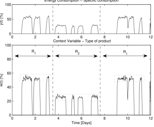
The purpose of this simulation is to illustrate de context identification concepts, ap-plied to an industrial plant, e.g. a milling unit, as depicted in figure 3.3.
In industrial milling units the different mixture of materials to be ground define the type of product under production. Depending on the mixture, the resulted blended ma-terial is more or less hard, which may require the re-circulation of mama-terial within the milling circuit in order to achieve a desirable level of narrowness, consuming more en-ergy in this process.
0 2 4 6 8 10 12
0 50 100
Energy Consumption − Specific consumption
y(t) [%]
0 2 4 6 8 10 12
0 20 40 60 80 100
Context Variable − Type of product
Time [Days]
w(t) [%]
R 2 R
1 R1
Therefore, in this case, the type of product being milled may be considered as a con-text variable. The flow of ground material a production variable and as a consumption measurement, consider the mill specific consumption1.
During the mill production time, two different types of product were produced. Prod-uct type 1, represented by an approximate constant value of 50%, was milled during the first 3 days, whereas product type 2, represented by approximately 25%, was milled be-tween the end of the 3th and the end of the 7th day. Afterwards, product type 1 was
under production again. Context regionR1defines the operating context when product
1 is under production, and context regionR2 for product type 2.
As it is depicted specific consumption shows quite different patterns when the oper-ating context changes. This is due to the type of product being produced. As the mixture of materials needed to mill product type 1 is harder that the mixture for product type 2, more energy is required for the milling process per unit of mass, as materials need to be re-circulated.
In order to carry out dynamically (while the plant is operating) the context and con-sumption identification, it is required a computational method able to automatically identify context regions, by finding its boundaries and calculate the average value of the context variable within the region, thus the centroid. Which drives this work to the next step: automatic context identification.
3.2
Automatic Context Identification
A way to define regions is by successively sub-divide, or partition, the context vari-able space into smaller groups until the resultant chunks are nearly steady constant over an average value or a certain period of steadiness is guaranteed. This method is called recursive partitioning. A well known and studied algorithm - Regression Trees (RT) is a suitable method for the partition of both continuous or categorical variable, which repre-sents the partition on a tree diagram.
3.2.1 Regression Tree Algorithm
The issue of finding structural breaks can be briefly described as follows [54, 55]. Consider that a context variablew(t)(either categorical or not), is characterized byL
context regions withL−1breaks, in whichw(t)can be approximated by a mean value. Hence, the partition ofw(t)is defined as:
w(t) =cRl+ξ(t), l= 1,· · ·, L (3.3)
Whereclis the centroid’s region,ξis the error term of the partition andtis the parti-tion of the time vector into regions as follows:
t=Tl−1+ 1 · · · Tl, l= 1,· · · , L (3.4) Assuming the conventionT0 = 0andTLis the series length.
The problem is to identify the set of unknown commutation points (i.e. boundaries) that best partition the context variable:
P(L) ={(1,· · · .T1),· · ·,(Tl−1+ 1,· · ·, Tl),· · · ,(TL−1+ 1,· · · , TL)} (3.5) Hence,P(L)defines the partition ofwintoLregions:
P(L) ={R1,· · · , Rl,· · ·, RL} (3.6) Where a regionRlis given by:
Rl= (Tl−1+ 1· · ·Tl) (3.7) One way to solve the problem is to use the least squares principle, so that the esti-mated regions:
ˆ
P(L) = ( ˆR1,· · · ,Rˆl,· · ·,RˆL) (3.8)
are such that:
ˆ
P(L) =argminPˆ(L)SSR(P(L)) (3.9)
Where the objective function SSR(P(L)), is the sum of squares residual (SSR),
de-fined by:
SSR(P(L)) = L X
l=1
X
t∈Rl
(w(t)−cRl)2 (3.10)
Andclis the mean value (centroid) ofw(t)over a regionRl.
cRl = X
t∈Rl
w(t)
Tl−(Tl−1+ 1)
(3.11)