Radiocarbon age offsets between two surface dwelling planktonic foraminifera
2
species during abrupt climate events in the SW Iberian margin
3
Blanca Ausín1, Negar Haghipour1, Lukas Wacker1, Antje H. L. Voelker2, 3, David Hodell4, 4
Clayton Magill5, Nathan Looser1, Stefano M. Bernasconi1, Timothy I. Eglinton1 5
1
Geological Institute, ETH Zürich, Zurich 8092 Switzerland 6
2
Centre of Marine Sciences (CCMAR), Universidade do Algarve, Faro 8005-139 Portugal 7
3
Instituto Português do Mar e da Atmosfera, 1495-006 Lisboa, Portugal 8
4
Department of Earth Sciences, University of Cambridge, Cambridge CB2 3EQ United 9
5
Lyell Centre, Heriot-Watt University, Edinburgh EH14 4AS United Kingdom 10
Kingdom 11
Corresponding author: Blanca Ausín (blanca.ausin@erdw.ethz.ch) 12
13
Key Points: 14
Leaching of the outer shell is a powerful diagnostic for external subtle contamination and 15
an effective tool to obtain more reliable radiocarbon dates. 16
Co-occurring planktonic foraminifera species sampled across abrupt climatic events show 17
radiocarbon age offsets of up to 1030 yr. 18
Differential bioturbation coupled with species abundance changes is invoked to explain 19
such temporal discrepancies. 20
Abstract 22
This study identifies temporal biases in the radiocarbon ages of the planktonic foraminifera 23
species Globigerina bulloides and Globigerinoides ruber (white) in a sediment core from the SW 24
Iberian margin (so-called ‘Shackleton site’). Leaching of the outer shell and measurement of the 25
radiocarbon content of both the leachate and leached sample enabled us to identify surface 26
contamination of the tests and its impact on their 14C ages. Incorporation of younger radiocarbon 27
on the outer shell affected both species and had a larger impact down-core. Inter-species 28
comparison of the 14C ages of the leached samples reveal systematic offsets with 14C ages for G. 29
ruber being younger than G. bulloides ages during the last deglaciation and part of the Early and
30
mid-Holocene. The greatest offsets (up to 1030 yr) were found during Heinrich Stadial 1 (HS1), 31
the Younger Dryas (YD), and part of the Holocene. The potential factors differentially affecting 32
these two planktonic species were assessed by complementary 14C, oxygen and carbon isotopes, 33
and species abundance determinations. The coupled effect of bioturbation with changes in the 34
abundance of G. ruber is invoked to account for the large age offsets. Our results highlight that 35
14
C ages of planktonic foraminifera might be largely compromised even in settings characterized 36
by high sediment accumulation rates. Thus, a careful assessment of potential temporal biases 37
must be performed prior to using 14C ages for paleoclimate investigations or radiocarbon 38
calibrations (e.g. marine calibration curve Marine13 (Reimer et al., 2013)). 39
1 Introduction 40
For decades, fossil planktonic foraminifera have been a valuable source of paleoceanographic 41
information, providing proxies for variations in ice-volume, sea level, salinity, temperature, and 42
nutrients (e.g. Pearson, 2012). Since the discovery of the radiocarbon (14C) dating technique in 43
the late forties (Libby et al., 1949), radiocarbon age determination of planktonic foraminifera has 44
become a cornerstone for paleoclimate investigations spanning the last 50,000 years. Most 45
studies rely on this method to build chronostratigraphic frameworks for marine sediment 46
sequences and constrain changes in thermohaline circulation by estimating radiocarbon 47
ventilation ages. However, prior works have demonstrated that planktonic foraminifera 14C ages 48
might not always be a reliable indicator of their depositional ages due to numerous causes, as 49
summarized by Mekik (2014). For instance, contamination trough radiocarbon addition by 50
secondary calcite precipitation or adhesion of atmospheric carbon, which can go unnoticed 51
during visual sample inspection under an optical microscope, can lead to large deviations in 14C 52
ages (Wacker et al., 2014; Wycech et al., 2016). Other possible causes of temporal biases include 53
bioturbation along with differential dissolution and fragmentation (Barker et al., 2007, and 54
references therein), differential bioturbation coupled with species abundance gradients (e.g. Bard 55
et al., 1987b), transport and deposition of reworked specimens (Broecker et al., 2006), and 56
distinct calcifying habitats (Lindsay et al., 2015). All these might differentially affect 57
foraminifera species and their influence on foraminifera 14C ages might be largely overlooked if, 58
as in most paleo-investigations, only samples of one species are analyzed per sediment horizon. 59
Thus, a more thorough assessment of the potential temporal biases between co-occurring 60
foraminifera species is required prior conducting investigations primarily based on climate 61
signals derived from foraminifera tests. Given age discrepancies might exceed the duration of 62
abrupt climate events (> 1,000 yr) (Mekik, 2014), important questions arise in relation to the 63
applicability of the latter approach in regions where marine sediments have a unique potential to 64
unravel rapid climate and environmental changes. 65
In this regard, The so-called Shackleton sites, MD95-2042 and IODP Site U1385, on the SW 66
Portuguese margin constitute benchmark cores for paleocenographic studies. For instance, Bard 67
et al. (2004) produced a down-core sequence of G. bulloides 14C ages in core MD95-2042, which 68
was incorporated into IntCal09/Marine09 (Reimer et al., 2009) and subsequent updates (Reimer 69
et al., 2013). This location has also emerged as one of the few regions in the world where direct 70
correlation of marine signals with both Greenland and Antarctic ice-core signals are feasible 71
(Shackleton et al., 2000), detailed chronostratigraphies have been developed (e.g. Bard et al., 72
1987a; Shackleton et al., 2004), and where ventilation and reservoir ages have been studied 73
(Skinner & Shackleton, 2004; Skinner et al., 2014), all these based on 14C ages of one species of 74
planktonic foraminifera per sediment horizon. 75
Despite the importance attached to this location and prior works posing severe pitfalls to 76
the latter approach, assessment of potential temporal biases trough 14C determinations on paired 77
species-specific samples has not yet been conducted. Consequently, potential temporal biases 78
might have been disregarded in derived paleoclimate interpretations from this key study area. We 79
aimed at identifying possible temporal biases in the 14C ages of planktonic foraminifera species, 80
analyzed in samples from a sediment core retrieved close to the location of IODP Site U1385, 81
and assessing the potential causes for age deviations. To accomplish this, we investigated paired 82
14
C ages of two of the most commonly used planktonic foraminifera species: Globigerina 83
bulloides and Globigerinoides ruber (white) and measured complementary oxygen (δ18O) and
84
carbon (δ13
C) isotopes, and species abundance data to elucidate possible reasons why 85
radiocarbon ages may diverge for different foraminifera species from the same sample. 86
2 Study area 87
The SW Iberian margin (NE Atlantic Ocean) is a transitional region where the Portugal Current 88
(PC), a branch of the North Atlantic Current, flows southward year-round (Fig. 1a) (Brambilla et 89
al., 2008; Pérez et al., 2001). From October to March, the Iberian Poleward Current (IPC), a 90
branch from the Azores Current, flows poleward along the W Portuguese margin (Haynes & 91
Barton, 1990). This shift in the near-shore surface circulation is linked to the seasonal changes in 92
the regional atmospheric circulation, which determine two well-differentiated oceanographic 93
regimes. From March/April to September/October, prevailing northeasterly winds may induce 94
Ekman transport offshore and subsequent upwelling of sub-surface waters. During the rest of the 95
year, coastal downwelling occurs under prevailing southwesterly winds (Peliz et al., 2005). 96
Upwelled sub-surface (100-500 m) waters consist in North Atlantic Central Water of either 97
subtropical (NACWst; 100-250 m) or subpolar (NACWsp; 250-500 m) origin. The warmer and 98
nutrient-poor NACWst overlies the colder, nutrient-richer NACWsp, which only upwells during 99
strong upwelling events. Below the NACW, the denser Mediterranean Outflow Water (MOW) 100
flows poleward between 500 and 1700 m. Below the intermediate waters, the Northeast Atlantic 101
Deep Water (NEADW) flows southward (van Aken, 2000), along with varying contributions of 102
the Upper Circumpolar Deep Water (UCDW), the Upper Labrador Sea Water (ULSW), and the 103
Antarctic Bottom Water (AABW) (Jenkins et al., 2015). 104
3 Materials and Methods 105
We analysed down-core sediment samples from kasten core SHAK06–5K (37°34′N, 10°09′W, 106
2,646 m), recovered by RSS James Cook during the cruise JC089 in 2013 in the vicinity of the 107
Shackleton Sites (Hodell et al., 2014). 108
3.1. Radiocarbon determinations 109
The majority of the organic matter contained in the initial sediment was extracted with organic 110
solvents following Ohkouchi et al. (2005) to use the organic fraction in a follow-up investigation. 111
To assess the possible influence of this procedure on the foraminifera contained in the solvent-112
extracted residue, we also analysed five samples of G. bulloides tests selected from non-113
extracted sediments. Between 15-30 g of dry sediment were diluted in MiliQ® water and 114
sonicated for only 15 seconds for disaggregation while avoiding shell fragmentation. The 115
solution was then wet-sieved through 300 µm and 250 µm mesh sieves and thoroughly washed 116
using a high-pressure stream of MiliQ® water. The resulting 250-300 µm size fraction was 117
immediately dried at 60°C overnight, prior to collecting 45-100 well-preserved shells of G. 118
bulloides or G. ruber from each sample. In some intervals, only 7-20 specimens of G. ruber were
119
available, limiting the amount of measured carbon (Tables S1 and S2). Radiocarbon 120
determinations (14C/12C) were performed with a gas ion source in a Mini Carbon Dating System 121
(MICADAS) at the Laboratory of Ion Beam Physics, ETH Zürich with an automated method for 122
acid digestion of carbonates whose sensitivity allows for less than10 µg of total carbon to be 123
measured (Wacker et al., 2013). The method is outlined as follows: vials (septa sealed 4.5 ml 124
exetainers vials from Labco Limited, UK) containing the samples were purged for 10 min with a 125
flow of 60 ml/min He to remove atmospheric CO2. Later, samples were briefly leached by 126
adding 100 µL of ultrapure HCl (0.02 M) with an automated syringe to remove possible surface 127
contaminants. The CO2 released from the leachate, referred to as “leachate” was transported by 128
helium to a zeolite trap and automatically injected into the ion source to be measured for 129
radiocarbon. The remaining sample, containing 12 µg C and referred to as “leached sample” was 130
subsequently acidified by adding 100 µL of ultrapure H3PO4 (85%) that was heated to 60°C for 131
at least 1 h. The released CO2 was loaded in a second trap and injected into the ion source to be 132
analyzed for radiocarbon (Wacker et al., 2014). Bard et al. (2015) showed that the F14C (fraction 133
modern according to Reimer et al. (2004)) of leachates from sequential leaching of discrete 134
samples converge towards a comparable value to that of the F14C of the leached sample (Bard et 135
al., 2015). Thus, we propose differences < 5 % between the two values as an indication of near-136
complete removal of surface contaminants. Five replicates of G. bulloides samples, referred to as 137
“untreated”, were directly measured without leaching the outer shell to assess the necessity of 138
this method. This gas ion source AMS system has a background 14C/12C value of F14C 0.0020+-139
0.0010 (50000 BP), determined on marble (IAEA-C1). Radiocarbon determinations were 140
corrected for isotopic fractionation via 13C/12C isotopic ratios and are given in conventional 141
radiocarbon ages. Radiocarbon ages and errors were not rounded to avoid artificial increments of 142
age offsets and propagated errors. 143
3.2. Age-depth model 144
The age depth model for core SHAK06–5K is a depositional model (P_Sequence type) based on 145
41 14C ages of monospecific samples of G. bulloides (Table 1) built with the calibration package 146
Oxcal(Bronk Ramsey, 2009). Conventional radiocarbon ages were calibrated to incorporate a 147
static marine reservoir effect using Marine13 curve (Reimer et al., 2013). The resulting age-148
depth model spans the last 28,000 years. 149
3.3. Scanning Electron Microscope (SEM) imagery 150
Representative well-preserved specimens were selected from discrete intervals to assess surface 151
preservation and possible early diagenetic overgrowth. Samples were graphite coated and SEM 152
images were generated using a JEOL JSM-6390LA digital SEM with a W filament. 153
3.4. Oxygen and carbon stable isotope analyses 154
Oxygen and carbon stable isotope analyses were determined every 2 cm when possible. In total, 155
164 samples of G. bulloides and 140 samples of G. ruber were considered. Between 6 and 12 156
specimens of each species were measured with a Gas Bench II connected to a Delta V Plus 157
isotope ratio mass spectrometer at the Stable Isotope Laboratory of Climate Geology, ETH 158
Zurich (Breitenbach & Bernasconi, 2011). Calibration to the VPDB scale was accomplished 159
using two in-house standards previously calibrated against the NBS-18 and NBS-19 international 160
standards. The associated long-term standard deviation is < 0.07‰. 161
3.5. Species abundance 162
Representative aliquots of the 250-300 µm size fraction, containing at least 300 planktonic 163
foraminifera shells, were obtained with a splitter. The relative and absolute abundances of G. 164
bulloides and G. ruber were analysed in 33 samples spaced every 10 cm. Absolute abundances
165
were calculated using the dry weight of the initial sieved sample. 166
4 Results 167
Radiocarbon ages of. G. bulloides samples from both extracted and non-extracted sediments 168
show younger leachates (up to 2000 yr) compared to the corresponding leached samples (Fig. 2, 169
Table 2). The leached samples from both types of sediments agree very well within their 1- σ 170
error. 171
The 5 untreated samples are younger than the paired leached samples and older than the leachate 172
(Fig. 3a). Age discrepancies among these three types of material measurements increase down-173
core. 174
Radiocarbon determinations generally reveal younger ages for the leachate in relation to the 175
corresponding leached samples for both species (Fig. 3a-b, Table 3). Leached samples display a 176
systematic aging down-core with few reversals of minimal magnitude. By contrast, 14C ages of 177
the leachate deviate from this trend, showing increasing variability down-core. While many of 178
the age offsets between leached samples and paired leachates within the top 90 cm fall into their 179
associated 1-σ uncertainty envelope, they show an apparent increase in magnitude down-core (up 180
to 1595-1660 yr for both species at 260 cm, and up to 4015 yr for G. bulloides at the bottom of 181
the core) (Fig. 3c, Table 3). Differences < 5 % between the F14C of leachates and corresponding 182
leached samples indicate near-complete removal of surface contaminants for all the samples 183
(Tables S1 and S2). Inter-species age differences of the leached sample reveal age offsets of up 184
to 1030 yr, and only three of them overlap within their associated 1-σ uncertainty (Fig. 3d, Table 185
3). G. bulloides ages are generally older than G. ruber ones, a pattern that is reversed for two 186
samples of the last glacial maximum, and within the top 20 cm of the core. The largest offsets 187
coincide with the occurrence of three abrupt climate events: the Heinrich Stadial 1 (HS1), 188
Younger Dryas (YD), and part of the Holocene (approximately 9-6 kyr). Limited material 189
prevented some samples to be leached and were measured as untreated samples. Three of these 190
G. ruber samples (280 cm, 270 cm, and a replicate of the latter) strongly deviate towards
191
younger ages. 192
4.1. SEM imagery 193
Overall, tests of both species exhibit good preservation with minor overgrowth (i.e., secondary 194
calcite) on the original base of the spines (Fig. S1). Such features are consistently observed in all 195
samples, irrespective of their depth interval. Both, G. bulloides and G. ruber show variable 196
amounts of coccoliths glued on the outer wall. Nevertheless, this feature does not affect all the 197
samples nor all the specimens, and there is no relationship between the presence nor the amount 198
of coccoliths and sample depth. 199
4.2. Isotopic composition of G. bulloides and G. ruber 200
Carbon isotopes of G. bulloides range between -0.4 and -1.8 ‰, and show higher values during 201
the cold intervals associated to the HS2, HS1 and YD, and part of the Holocene (Fig. 4b). The 202
δ13
C data of G. ruber vary between 1.4 and -0.4 ‰ and show relatively constant values for the 203
first half of the record (340-170 cm) and an increasing trend towards more positive values 204
thorough the Holocene. Oxygen isotopes of G. bulloides range between 0.1-3.0 ‰ and record 205
short-term isotopic changes associated with HS2, HS1 and YD (Fig. 4c). The δ18O data of G. 206
ruber range between -0.1 and 2.2 ‰. This record shows a smoother profile than that of G.
207
bulloides and lacks samples for part of HS1. Both isotopic curves are out-of-phase by at least 10
208
cm for most of the last deglaciation (70-140 cm). The oxygen isotopic difference between both 209
species (Δδ18
Ob-r) ranges from –0.3 ‰ to 1.7 ‰ and shows highest values during the HS2, HS1, 210
and YD (Fig. 3c). 211
4.3. Variation in species abundances 212
Average absolute and relative abundances of G. bulloides are 6 specimens g-1 and 24%, 213
respectively, and show large increases during the cold intervals HS2, HS1, and the YD (up to 25 214
specimens g-1 and 72%) (Fig. 4e). G. ruber shows average absolute and relative abundances of 1 215
specimens g-1 and 4%. This species is almost absent during HS2, HS1 and YD, and increases to 216
up to 8 specimens g-1 and 13% during the late Holocene (top 30 cm). 217
5 Discussion 218
5.1. Contamination through secondary radiocarbon addition: the need for a leaching step 219
Age discrepancies between paired leached samples and leachates highlight the secondary 220
addition of younger carbon and subsequent contamination on the outer shell (Fig. 3a and b, Table 221
3), as observed by previous authors when applying similar leaching steps (Bard et al., 2015). 222
Such contamination was not introduced by using organic solvents for lipid extraction, as the 223
leachates were always younger than corresponding leached samples, regardless of whether 224
foraminifera come from solvent-extracted or non-extracted sediments (Fig. 2, Table 2). The 225
magnitude of such age discrepancy does not always agree for both methods, but this can be 226
explained by the varying and small amounts of C measured from the leachate (Table S1). 227
Moreover, comparison of 14C ages of leached samples from both types of sediments show 228
negligible differences (Fig. 2). These results are in line with previous findings of Ohkouchi et al. 229
(2005), who concluded that tests from solvent-extracted sediments can be reliably used for 14C 230
determinations. Additional influence of other sample preparation steps cannot be fully discarded. 231
For instance, soaking of foraminifera during wet sieving can activate their reactive surface and 232
enable adhesion of ambient carbon. However, we minimized the potential influence of this 233
process by drying the samples in the oven right after sieving. Another possibility to consider is 234
the influence of early diagenesis. Minor signs of secondary calcite precipitation are apparent by 235
SEM imagery in all the tests (Fig. S1), regardless of sample depth and species. Diagenetic 236
alteration of shells through ∑CO2 exchange with pore waters with a younger 14C signature might 237
explain the negligible impact of secondary calcite precipitation on samples from the top 60 cm 238
and the more variable and larger effect observed down-core (Fig. 3c). These results highlights 239
the need of a leaching step to remove surface contaminants, especially for older samples, for 240
which age biases can be greater than 1000 yr (Fig. 1a, Table 3). 241
Regarding the untreated samples of G. ruber, two large deviations toward younger-than-expected 242
ages are also evident at the bottom of the core (Fig. 3b). Within single depth horizons of a core 243
retrieved from the Portuguese margin, Löwemark and Grootes (2004) found large intra-species 244
age discrepancies (up to 2590 years) when comparing sediments affected and unaffected by trace 245
fossils indicating bioturbating organisms (e.g., Zoophycos). Because ichnofossils occur 246
throughout the sediments of IODP Site U1385 (Tovar & Dorador, 2014; Rodríguez-247
Tovar et al., 2015), they most certainly also affect the sediments of core SHAK06–5K. Their 248
influence would imply that discrete samples from the same sediment horizon would consist of a 249
mixture in different proportions of foraminifera tests from both bioturbated and non-bioturbated 250
material. The excellent agreement between the two replicates of G. ruber samples from depth 251
horizon 270 cm excludes bioturbation as the reason for such age deviations. Addition of younger 252
secondary calcite might also explain these age deviations, although lack of material prevented 253
further assessment. 254
5.2. Inter-species radiocarbon age differences 255
Assuming removal of the majority of external contamination by the leaching step (Table S1), 256
secondary radiocarbon addition does not account for the 14C age differences between the leached 257
samples of the two species (Fig. 3d), and mechanism(s) differentially affecting foraminifera 258
species must be sought to explain the systematic younger-than-G. bulloides 14C ages for G. 259
ruber. Ideally, such mechanism(s) should also explain changes in the magnitude of the observed
260
age offsets with abrupt climate events. In the following, we discuss four possible mechanisms. 261
5.2.1. Contrasting calcifying habitats 262
Differences in calcifying depth and season of the two species might have also played a role in 263
14
C age discrepancies. Mollenhauer (1999) demonstrated that inter-species differences of 540 264
years are possible in upwelling settings, where deep, less-ventilated, “older” waters are upwelled 265
to the surface. Currently in the study area, the average living depths (ALD) of G. ruber and G. 266
bulloides are 58±6 and 102±21 m, respectively (Rebotim et al., 2017). While G. ruber is
267
characteristic of winter hydrographic conditions, G. bulloides is more abundant during the 268
upwelling season (i.e., summer) (Salgueiro et al., 2008). Figure 5 shows the natural radiocarbon 269
content (Δ14
C) depth profile from a station corresponding to the water column overlying the 270
depositional area of the study site, extracted from the Global Ocean Data Analysis Project 271
(GLODAP) (Key et al., 2004). Corresponding natural Δ14C values for ALD of G. ruber and G. 272
bulloides are -59 ‰ and ~ -65 ‰, respectively, equivalent to an age discrepancy of ~50 yr,
273
which is insufficient to explain age offsets between species. As seasonality also impacts on the 274
optimal conditions for G. ruber and G. bulloides proliferation, we calculated the winter and 275
summer natural Δ14
C for the upper 500 m of the water column. We applied the linear relationship 276
between natural Δ14C and dissolved silicate for North Atlantic latitudes (equation (1)) proposed 277
by Broecker et al. (1995), using summer and winter dissolved silicate estimates (García et al., 278
2014) averaged at 100 and 60 m water depth, respectively, from the 2013 World Ocean Atlas 279
(WOA13). 280
Natural Δ14C = –60 – dissolved silicate in µmol/kg (1) 281
Yet, the estimated seasonal difference in Δ14C is minimal (-3.2 ‰) and negligible in relation to 282
the large uncertainty derived from the silicate method (±15 ‰) (Rubin & Key, 2002). 283
However, it is still possible that the associated radiocarbon reservoirs (or at least one of them) 284
varied in the past during HS1, YD, and part of the Holocene related to the large hydrographic 285
changes that occurred during abrupt climate events in the study area (Voelker & de Abreu, 286
2011). This argument was put forward by Löwemark and Grootes (2004) to explain the large age 287
discrepancy they found between G. bulloides and G. ruber during the YD on the Portuguese 288
margin. In this regard, the incursion of intermediate, extremely 14C–depleted waters 289
characterized by high nutrient content has been suggested to reach latitudes as far as 60°N in the 290
Atlantic during the abrupt cold intervals HS1 and YD (Pahnke et al., 2008; Rickaby & 291
Elderfield, 2005; Thornalley et al., 2011). The authors pointed to Antarctic Intermediate Water 292
(AAIW), which would have extended northward as a consequence of Atlantic Meridional 293
Overturning Circulation (AMOC) weakening or collapse. Indeed, such drastic reductions of 294
AMOC during HS1 and YD prevented the formation of new North Atlantic Deep Water 295
(NADW) (McManus et al., 2004), which would have then been replaced by AAIW. However, 296
the hypothesis of markedly different radiocarbon reservoirs affecting each of the species is not 297
fully supported by other data. G. ruber δ13C values give no clear indication of upwelling of 298
nutrient-rich waters occurring during HS2 or YD, and lack of G. ruber during HS1 prevents 299
further interpretation (Fig. 4b). More positive δ13C values of G. bulloides rather suggest that 300
upwelling had decreased at those times. Although less negative δ13C values could also be the 301
result of upwelling and subsequent nutrient consumption by primary producers, resulting in a 302
13
C-enrichment of surrounding waters, this scenario disagrees with previous studies. Estimates of 303
export production by (Salgueiro et al., 2010) and of primary productivity and upwelling 304
occurrence by (Incarbona et al., 2010) are best explained with the arrival of freshwater during 305
HS1 and YD resulting in water column stratification, decreased upwelling and a large drop in 306
productivity. Moreover, assuming that the general ecological preferences of each species 307
remained constant during the last deglaciation, upwelling of AAIW would preferentially affect 308
G. bulloides. Yet, radiocarbon ages corresponding to the δ18O excursions of G. bulloides 309
associated with HS2, HS1 and YD are in very good agreement with the established age ranges 310
for these abrupt climate events (Fig. S2), which underpins the notion that G. bulloides 14C ages 311
are not, at least severely, biased in relation to their depositional ages. Additionally, we believe 312
this mechanism fails to explain temporal discrepancies during the Holocene. Even though a 313
relative increase of AAIW influence in higher northern latitudes can be recognized from 314
neodymium isotope ratios (Pahnke et al., 2008), there is no evidence of a large reduction of 315
AMOC at that time, which is believed to have been relatively strong during the Holocene 316
(Gherardi et al., 2005; Thornalley et al., 2011). Although we cannot completely refute that the 317
influence of water masses with distinct radiocarbon content (Δ14C) contributed to the observed 318
age offsets during HS1 and YD, an additional mechanism is needed to explain the smoothed 319
δ18
O curve of G. ruber in relation to that of G. bulloides (Fig. 4c) a feature typical of bioturbated 320
sediment (Bard et al., 1987a). 321
5.2.2. The Barker effect 322
The Barker effect (first proposed by Andree et al. (1984), Peng & Broecker (1984), Broecker 323
et al. (1984), and Broecker et al. (2006) and coined by Broecker and Clark (2011), refers to the 324
differential effect of partial dissolution and subsequent fragmentation of shells along with 325
bioturbation on the 14C ages of different species planktonic foraminifera (Barker et al., 2007; 326
Broecker & Clark, 2011). Given that different species may dissolve at different rates, fragile and 327
dissolution-prone species (i.e., G. ruber) will fragment in the sediment mixed layer more easily 328
than more robust, dissolution-resistant species (i.e., G. bulloides) (Berger, 1968; 1970). This 329
translates into shorter residence times in the sediment for G. ruber relative to G. bulloides. 330
Consequently, the pool of non-fragmented shells of G. ruber at a given horizon will be biased 331
towards younger specimens, because specimens that reside in the bioturbated layer for longer 332
periods are more likely to be fragmented. As only well-preserved whole tests were picked for 14C 333
analyses, monospecific samples of G. ruber will be, on average, younger than G. bulloides. 334
This effect was invoked to account for age discrepancies among planktonic foraminifera 335
species of up to several thousand years especially in cores characterized by low sediment 336
accumulation rates (< 3 cm/kyr) (Barker et al., 2007; Broecker et al., 2006; Broecker & Clark, 337
2011; Peng & Broecker, 1984). The latter is an important factor to be taken into account since 338
the lower the sedimentation rate, the longer the exposure time to the effect of bioturbation. High 339
sedimentation rates of core SHAK06–5K only decrease to a minimum of 6 cm/kyr for the 340
interval from 80 to 50 cm (Fig. 4a). However, the observed apparent increase in the inter-specific 341
14
C age offset is not exclusive to this horizon and visual inspection of nannofossils confirmed 342
their excellent preservation thorough the Holocene. 343
Yet, highly productive settings may have favored acidification of underlying waters and pore 344
waters through CO2 release by respiration. Despite being part of a major upwelling system, total 345
organic content in core SHAK06–5K and broader region (Baas et al., 1997; Magill et al., 2018) 346
ranges from only 0.2 to 0.7 % for the whole studied period, suggesting that substantial 347
dissolution by organic carbon oxidation is unlikely. Similarly, changes in the depth of the calcite 348
lysocline are also assumed to have had a negligible effect, because the water depth of the core 349
(2578 m) is located well above that level. Influence of more corrosive water masses could have 350
promoted increased dissolution of G. ruber. However, incursion of southern sourced water-mass 351
was mostly limited to glacial periods (Skinner & Shackleton, 2004), characterized by relatively 352
high sedimentation rates. Therefore, we consider it is unlikely that the Barker effect had a major 353
influence in the observed 14C age discrepancies between foraminifera species. 354
5.2.3. Lateral and along-slope transport 355
Introduction of reworked specimens by advection and along-slope sedimentary processes could 356
also contribute to radiocarbon age discrepancies, a mechanism proposed in cores from the 357
Eastern Equatorial Pacific, the Mid-Atlantic Ridge, and the South China Sea (Broecker et al., 358
2006). Addition of reworked calcareous nannofossils by lateral transport has been observed in 359
the study area (Incarbona et al., 2010) and in core SHAK06–5K (Magill et al., 2018), especially 360
during HS1. Simulated bottom velocities in the study area might locally exceed 10 cm/s, able to 361
transport dense, 250-300 µm sized grains of foraminifera when locally reaching >40 cm/s 362
(Hernández-Molina et al., 2011). To explain the observed older-than-G. ruber ages for G. 363
bulloides by any of these mechanisms, transport and deposition of large numbers of reworked
364
(old) G. bulloides would be necessary, along with preferential fragmentation of G. ruber during 365
transport. This might be a feasible scenario, albeit it would imply that samples of G. bulloides 366
are the ones affected by a temporal bias between biosynthesis and deposition. We thus discard 367
this hypothesis based on: (i) the good agreement of G. bulloides δ18O excursions during short-368
term climate changes and their associated established age ranges (Fig. S2) and (ii) the smoothed 369
δ18
O curve of G. ruber that hardly resolves the major abrupt climate events occurred the last 370
deglaciation (Fig. 4c). Such results suggest that G. ruber, rather than G. bulloides, accounts for 371
the age offsets between the two species. 372
5.2.4. Differential bioturbation coupled with changes in species abundances 373
The joint effect of downward mixing of foraminifera due to bioturbation and changes in their 374
abundance might promote 14C offsets between species (Andree et al., 1984; Bard et al., 1987a; 375
Broecker et al., 1999; Broecker et al., 1984; Peng & Broecker, 1984). Foraminifera will always 376
be mixed from a horizon of high abundance to low abundance. Given an increase (decrease) in 377
the abundance of a certain species in a sediment horizon, bioturbation is expected to down-mix 378
(up-mix) some of these “young” (“old”) foraminifera. As a result, the horizon underneath (above 379
it) will be enriched in younger (older) specimens, leading to corresponding deviations in their 380
expected 14C ages. The clear aging trend with depth gives no indication of homogenization by 381
bioturbation > 10 cm (Figs. 2a and b). However, the δ18O record of G. ruber lags that of G. 382
bulloides by 10 cm during the HS1, last deglaciation, and YD (Fig. 4d). This shift is more
383
apparent when comparing samples at lower resolution (every 10 cm only) (Figure S3) and 384
suggests a mixed layer depth equivalent to ≤ 10 cm. Similar out-of-phase relationships between 385
species-specific isotopic records have previously been explained through this mechanism (Bard 386
et al., 1987a; Bard et al., 1987b; Hutson, 1980). Löwemark and Grootes (2004) also invoked it to 387
account for differences of 75-350 years between G. bulloides and G. ruber in a nearby core from 388
the SW Portuguese margin. According to these authors, and given the large changes in the 389
abundance of G. bulloides relative to those of G. ruber (Fig. 4e), a larger impact on the 14C ages 390
of the former species would be expected. This hypothesis is difficult to reconcile with the 391
smoothed δ18O curve of G. ruber. We would expect G. ruber to be the species more affected by 392
differential bioturbation than G. bulloides. Indeed, and with the exception of the sample at 60 393
cm, each large increase in Δδ18O is followed by a rise in G. ruber absolute abundance (Figs. 3c 394
and d) that, despite their moderate magnitude, also follow periods of extremely low abundance or 395
near absence. Our data is a faithful reproduction of previous mathematical simulations of Trauth 396
(2013) and Bard et al. (1987a), who demonstrated the effects of bioturbation coupled with 397
abundance changes in the oxygen isotopic record of a “warm” species (i.e., G. ruber) during 398
deglaciation (see figure 4 in Bard et al., 1987a). Our results do not agree well with their model 399
for the “cold” species (i.e., G. bulloides) because they are permanently present, and 400
“authoctonous” specimens can make up for the radiocarbon addition from foraminifera 401
belonging to adjacent sediment horizons. 402
6 Conclusions 403
Radiocarbon dates of paired monospecific samples of G. bulloides and G. ruber (white) were 404
determined in marine sediments retrieved from the SW Iberian Margin. 14C age differences of 405
several thousands of years between paired leachates and leached samples indicate addition of 406
younger radiocarbon in both species. This process is attributed to precipitation of younger 407
secondary calcite by ∑CO2 exchange with 14C-rich pore waters and/or ambient carbon adhesion 408
during sample sieving, thus having a more variable and greater impact down-core. Leaching of 409
the outer shell has proven to be a powerful diagnostic for external contamination, and more 410
importantly, a tool to obtain more reliable radiocarbon dates, especially when dealing with older 411
samples (>10 kyr). Our findings underscore the need to properly leach foraminiferal samples 412
prior to radiocarbon dating. 413
Inter-species age discrepancies of the leached samples ranged between 60 and 1030 years. G. 414
ruber yielded younger ages than paired G. bulloides in the same sample throughout most of the
415
record. Larger age discrepancies were found during HS1, YD, and part of the Holocene, and 416
were attributed to the effects of bioturbation coupled with species abundance changes. This 417
mechanism has a greater impact if the species in question has periods of absence (i.e., G. ruber) 418
rather than greater abundance changes (i.e., G. bulloides) because the population of rarer species 419
is more affected by the addition of asynchronous foraminifera compared to a more abundant 420
species. This process alone appears to provide a satisfactory explanation for the observed age 421
offsets, although additional influences such as past variations in the 14C reservoirs of the 422
respective calcifying habitats cannot be fully ruled out. 423
After a careful evaluation of potential 14C age anomalies in these two species, we conclude that, 424
unlike G. ruber, G. bulloides can be reliably used to develop foraminifera-based 14C age 425
chronostratigraphies and to assess ocean ventilation ages in the study area. 426
427
Author contribution 428
B.A. and T.I.E. planned this investigation. N.H. and L.W. assisted with radiocarbon analyses. 429
N.L. assisted with SEM imagery. B.A. prepared the samples, analyzed the results and wrote the 430
manuscript with contributions by all co-authors. 431
432
Acknowledgements and Data 433
We thank two anonymous reviewers for their valuable contribution to improve this manuscript. 434
We would like to thank M. Jaggi for her assistance during isotope analyses. This study was 435
supported by an ETH Zurich Postdoctoral Fellowship from the Swiss Federal Institute of 436
Technology in Zurich (ETHZ) and the project 200021_175823 funded by Swiss National 437
Science Foundation, both granted to B.A. A.H.L.V. acknowledges financial support from the 438
Portuguese FCT through grants IF/01500/2014 and CCMAR (UID/Multi/04326/2013). The core 439
for this study was collected during Cruise 089 aboard the RSS James Cook that was made 440
possible with support from the UK Natural Environmental Research Council (NERC Grant 441
NE/J00653X/1). 442
All original data used in this study, necessary to understand, evaluate and replicate this research 443
is presented and available in tables within the main text and supporting information and it will be 444
equally available in the public repository PANGAEA®. 445
446
References 447
Andree, M., Beer, J., Oeschger, H., Broecker, W., Mix, A., Ragano, N., . . . Wölfli, W. (1984). 448
14C measurements on foraminifera of deep sea core V28-238 and their preliminary 449
interpretation. Nuclear Instruments and Methods in Physics Research Section B: Beam 450
Interactions with Materials and Atoms, 5(2), 340-345. doi:
https://doi.org/10.1016/0168-451
583X(84)90539-1
452
Baas, J. H., Mienert, J., Abrantes, F., & Prins, M. A. (1997). Late Quaternary sedimentation on 453
the Portuguese continental margin: climate-related processes and products. 454
Palaeogeography, Palaeoclimatology, Palaeoecology, 130(1), 1-23.
455
doi:https://doi.org/10.1016/S0031-0182(96)00135-6
456
Bard, E., Arnold, M., Duprat, J., Moyes, J., & Duplessy, J.-C. (1987a). Reconstruction of the last 457
deglaciation: deconvolved records of δ18O profiles, micropaleontological variations and 458
accelerator mass spectrometric14C dating. Climate Dynamics, 1(2), 101-112. 459
doi:10.1007/bf01054479 460
Bard, E., Arnold, M., Duprat, J., Moyes, J., & Duplessy, J. C. (1987b). Bioturbation Effects on 461
Abrupt Climatic Changes Recorded in Deep Sea Sediments. Correlation between δ18O 462
Profiles and Accelerator 14C Dating. In W. H. Berger & L. D. Labeyrie (Eds.), Abrupt 463
Climatic Change: Evidence and Implications (pp. 263-278). Dordrecht: Springer
464
Netherlands. 465
Bard, E., Rostek, F., & Ménot-Combes, G. (2004). Radiocarbon calibration beyond 20,000 14C 466
yr B.P. by means of planktonic foraminifera of the Iberian Margin. Quaternary Research, 467
61(2), 204-214. doi:https://doi.org/10.1016/j.yqres.2003.11.006
468
Bard, E., Tuna, T., Fagault, Y., Bonvalot, L., Wacker, L., Fahrni, S., & Synal, H. A. (2015). 469
AixMICADAS, the accelerator mass spectrometer dedicated to C-14 recently installed in 470
Aix-en-Provence, France. Nucl Instrum Meth B, 361, 80-86. 471
Barker, S., Broecker, W., Clark, E., & Hajdas, I. (2007). Radiocarbon age offsets of foraminifera 472
resulting from differential dissolution and fragmentation within the sedimentary 473
bioturbated zone. Paleoceanography, 22(2). doi:doi:10.1029/2006PA001354 474
Berger, W. H. (1968). Planktonic Foraminifera: selective solution and paleoclimatic 475
interpretation. Deep Sea Research and Oceanographic Abstracts, 15(1), 31-43. 476
doi:https://doi.org/10.1016/0011-7471(68)90027-2
477
Berger, W. H. (1970). Planktonic Foraminifera: Selective solution and the lysocline. Marine 478
Geology, 8(2), 111-138. doi:https://doi.org/10.1016/0025-3227(70)90001-0
479
Brambilla, E., Talley, L. D., & Robbins, P. E. (2008). Subpolar Mode Water in the northeastern 480
Atlantic: 2. Origin and transformation. Journal of Geophysical Research: Oceans, 481
113(C4). doi:doi:10.1029/2006JC004063
482
Breitenbach, S. F. M., & Bernasconi, S. M. (2011). Carbon and oxygen isotope analysis of small 483
carbonate samples (20 to 100 µg) with a GasBench II preparation device. Rapid 484
Communications in Mass Spectrometry, 25(13), 1910-1914. doi:doi:10.1002/rcm.5052
485
Broecker, W., Barker, S., Clark, E., Hajdas, I., & Bonani, G. (2006). Anomalous radiocarbon 486
ages for foraminifera shells. Paleoceanography, 21(2). doi:doi:10.1029/2005PA001212 487
Broecker, W., & Clark, E. (2011). Radiocarbon‐age differences among coexisting planktic 488
foraminifera shells: The Barker Effect. Paleoceanography, 26(2). 489
doi:doi:10.1029/2011PA002116 490
Broecker, W., Matsumoto, K., & Clark, E. (1999). Radiocarbon age differences between 491
coexisting foraminiferal species. Paleoceanography, 14(4), 431-436. 492
doi:doi:10.1029/1999PA900019 493
Broecker, W., Mix, A., Andree, M., & Oeschger, H. (1984). Radiocarbon measurements on 494
coexisting benthic and planktic foraminifera shells: potential for reconstructing ocean 495
ventilation times over the past 20 000 years. Nuclear Instruments and Methods in Physics 496
Research Section B: Beam Interactions with Materials and Atoms, 5(2), 331-339.
497
doi:https://doi.org/10.1016/0168-583X(84)90538-X
498
Broecker, W. S., Sutherland, S., Smethie, W., Peng, T. H., & Ostlund, G. (1995). Oceanic 499
radiocarbon: Separation of the natural and bomb components. Global Biogeochemical 500
Cycles, 9(2), 263-288. doi:doi:10.1029/95GB00208
501
Bronk Ramsey, C. (2009). Bayesian Analysis of Radiocarbon Dates. Radiocarbon, 51(1), 337-502
360. doi:10.1017/S0033822200033865 503
García, H. E., Locarnini, R. A., Boyer, T. P., Antonov, J. I., Baranova, O. K., Zweng, M. M., . . . 504
Johnson, D. R. (2014). World Ocean Atlas 2013, Volume 4: Dissolved Inorganic 505
Nutrients (phosphate, nitrate, silicate). In S. Levitus & A. Mishonov (Eds.), NOAA Atlas 506
NESDIS 76 (pp. 25).
507
Gherardi, J. M., Labeyrie, L., McManus, J. F., Francois, R., Skinner, L. C., & Cortijo, E. (2005). 508
Evidence from the Northeastern Atlantic basin for variability in the rate of the meridional 509
overturning circulation through the last deglaciation. Earth and Planetary Science 510
Letters, 240(3–4), 710-723. doi:http://dx.doi.org/10.1016/j.epsl.2005.09.061
511
Haynes, R., & Barton, E. D. (1990). A poleward flow along the Atlantic coast of the Iberian 512
peninsula. Journal of Geophysical Research: Oceans, 95(C7), 11425-11441. 513
doi:10.1029/JC095iC07p11425 514
Hernández-Molina, F. J., Serra, N., Stow, D. A. V., Llave, E., Ercilla, G., & Van Rooij, D. 515
(2011). Along-slope oceanographic processes and sedimentary products around the 516
Iberian margin. Geo-Marine Letters, 31, 315-341. 517
Hodell, D. A., Elderfield, H., Greaves, M., McCave, I. N., Skinner, L., Thomas, A., & White, N. 518
(2014). The JC089 scientific party, JC089 cruise report - IODP site survey of the 519
Shackleton sites, SW iberian margin, British ocean data Centre.
520
https://www.bodc.ac.uk/data/information_and_inventories/cruise_inventory/report/13392
521
/. Retrieved from
522
Hutson, W. H. (1980). Bioturbation of deep-sea sediments: oxygen isotopes and stratigraphic 523
uncertainty. Geology, 8, 127-130. 524
Incarbona, A., Martrat, B., Di Stefano, E., Grimalt, J. O., Pelosi, N., Patti, B., & Tranchida, G. 525
(2010). Primary productivity variability on the Atlantic Iberian Margin over the last 526
70,000 years: Evidence from coccolithophores and fossil organic compounds. 527
Paleoceanography, 25(2), PA2218, doi:2210.1029/2008PA001709.
528
Jenkins, W. J., Smethie, W. M., Boyle, E. A., & Cutter, G. A. (2015). Water mass analysis for 529
the U.S. GEOTRACES (GA03) North Atlantic sections. Deep Sea Research Part II: 530
Topical Studies in Oceanography, 116, 6-20.
531
Key, R. M., Kozyr, A., Sabine, C. L., Lee, K., Wanninkhof, R., Bullister, J. L., . . . Peng, T. H. 532
(2004). A global ocean carbon climatology: Results from Global Data Analysis Project 533
(GLODAP). Global Biogeochemical Cycles, 18(4). doi:doi:10.1029/2004GB002247 534
Libby, W. F., Anderson, E. C., & Arnold, J. R. (1949). Age Determination by Radiocarbon 535
Content: World-Wide Assay of Natural Radiocarbon. Science, 109, 227-228. 536
doi:10.1126/science.109.2827.227 537
Lindsay, C. M., Lehman, S. J., Marchitto, T. M., & Ortiz, J. D. (2015). The surface expression of 538
radiocarbon anomalies near Baja California during deglaciation. Earth and Planetary 539
Science Letters, 422, 67-74. doi:https://doi.org/10.1016/j.epsl.2015.04.012
Löwemark, L., & Grootes, P. M. (2004). Large age differences between planktic foraminifers 541
caused by abundance variations and Zoophycos bioturbation. Paleoceanography, 19(2). 542
doi:doi:10.1029/2003PA000949 543
Magill, C. R., Ausín, B., Wenk, P., McIntyre, C., Skinner, L., Martínez-García, A., . . . Eglinton, 544
T. I. (2018). Transient hydrodynamic effects influence organic carbon signatures in 545
marine sediments. Nature Communications, 9(1), 4690. doi:10.1038/s41467-018-06973-546
w 547
McManus, J. F., Francois, R., Gherardi, J. M., Keigwin, L. D., & Brown-Leger, S. (2004). 548
Collapse and rapid resumption of Atlantic meridional circulation linked to deglacial 549
climate changes. Nature, 428, 834. doi:10.1038/nature02494 550
https://www.nature.com/articles/nature02494#supplementary-information
551
Mekik, F. (2014). Radiocarbon dating of planktonic foraminifer shells: A cautionary tale. 552
Paleoceanography, 29(1), 13-29. doi:doi:10.1002/2013PA002532
553
Mollenhauer, G. (1999). Einfluß von Bioturbation, Produktivität und Zirkulation auf 14C-554
Datierungen an planktonischen Foraminiferen. (M.S.), University of Bremen.
555
Ohkouchi, N., Eglinton, T. I., Hughen, K. A., Roosen, E., & Keigwin, L. D. (2005). Radiocarbon 556
Dating of Alkenones from Marine Sediments: III. Influence of Solvent Extraction 557
Procedures on 14C Measurements of Foraminifera. Radiocarbon, 47(3), 425-432. 558
doi:10.1017/S0033822200035207 559
Pahnke, K., Goldstein, S. L., & Hemming, S. R. (2008). Abrupt changes in Antarctic 560
Intermediate Water circulation over the past 25,000 years. Nature Geoscience, 1, 870. 561
doi:10.1038/ngeo360 562
https://www.nature.com/articles/ngeo360#supplementary-information
563
Pearson, P. N. (2012). Oxygen Isotopes in Foraminifera: Overview and Historical Review. The 564
Paleontological Society Papers, 18, 1-38. doi:10.1017/S1089332600002539
565
Peliz, Á., Dubert, J., Santos, A. M. P., Oliveira, P. B., & Le Cann, B. (2005). Winter upper ocean 566
circulation in the Western Iberian Basin—Fronts, Eddies and Poleward Flows: an 567
overview. Deep Sea Research Part I: Oceanographic Research Papers, 52(4), 621-646. 568
doi:http://dx.doi.org/10.1016/j.dsr.2004.11.005
569
Peng, T.-H., & Broecker, W. S. (1984). The impacts of bioturbation on the age difference 570
between benthic and planktonic foraminifera in deep sea sediments. Nuclear Instruments 571
and Methods in Physics Research Section B: Beam Interactions with Materials and
572
Atoms, 5(2), 346-352. doi:https://doi.org/10.1016/0168-583X(84)90540-8
573
Pérez, F. F., Castro, C. G., Álvarez–Salgado, X. A., & Rı́os, A. F. (2001). Coupling between the 574
Iberian basin — scale circulation and the Portugal boundary current system: a chemical 575
study. Deep Sea Research Part I: Oceanographic Research Papers, 48(6), 1519-1533. 576
doi:https://doi.org/10.1016/S0967-0637(00)00101-1
577
Rebotim, A., Voelker, A. H. L., Jonkers, L., Waniek, J. J., Meggers, H., Schiebel, R., . . . Kucera, 578
M. (2017). Factors controlling the depth habitat of planktonic foraminifera in the 579
subtropical eastern North Atlantic. Biogeosciences, 14(4), 827-859. doi:10.5194/bg-14-580
827-2017 581
Reimer, P. J., Baillie, M. G. L., Bard, E., Bayliss, A., Beck, J. W., Blackwell, P. G., . . . 582
Weyhenmeyer, C. E. (2009). IntCal09 and Marine09 radiocarbon age calibration curves, 583
0-50,000 years cal BP. Radiocarbon, 51, 1111-1150. 584
Reimer, P. J., Bard, E., Bayliss, A., Beck, J. W., Blackwell, P. G., Bronk Ramsey, C., . . . van der 585
Plicht, J. (2013). IntCal13 and Marine13 Radiocarbon Age Calibration Curves 0-50,000 586
Years cal BP. Radiocarbon. Radiocarbon, 55. 587
Reimer, P. J., Brown, T. A., & Reimer, R. W. (2004). Discussion: Reporting and Calibration of 588
Post-Bomb 14C Data. Radiocarbon, 46(3), 1299-1304. doi:10.1017/S0033822200033154 589
Rickaby, R. E. M., & Elderfield, H. (2005). Evidence from the high-latitude North Atlantic for 590
variations in Antarctic Intermediate water flow during the last deglaciation. 591
Geochemistry, Geophysics, Geosystems, 6(5). doi:doi:10.1029/2004GC000858
592
Rodríguez-Tovar, F. J., & Dorador, J. (2014). Ichnological analysis of Pleistocene sediments 593
from the IODP Site U1385 “Shackleton Site” on the Iberian margin: Approaching 594
paleoenvironmental conditions. Palaeogeography, Palaeoclimatology, Palaeoecology, 595
409, 24-32. doi:https://doi.org/10.1016/j.palaeo.2014.04.027
596
Rodríguez-Tovar, F. J., Dorador, J., Grunert, P., & Hodell, D. (2015). Deep-sea trace fossil and 597
benthic foraminiferal assemblages across glacial Terminations 1, 2 and 4 at the 598
“Shackleton Site” (IODP Expedition 339, Site U1385). Global and Planetary Change, 599
133, 359-370. doi:https://doi.org/10.1016/j.gloplacha.2015.05.003
600
Rubin, S. I., & Key, R. M. (2002). Separating natural and bomb‐produced radiocarbon in the 601
ocean: The potential alkalinity method. Global Biogeochemical Cycles, 16(4), 52-51-52-602
19. doi:doi:10.1029/2001GB001432 603
Salgueiro, E., Voelker, A., Abrantes, F., Meggers, H., Pflaumann, U., Lončarić, N., . . . Wefer, 604
G. (2008). Planktonic foraminifera from modern sediments reflect upwelling patterns off 605
Iberia: Insights from a regional transfer function. Marine Micropaleontology, 66(3–4), 606
135-164. doi:http://dx.doi.org/10.1016/j.marmicro.2007.09.003
607
Salgueiro, E., Voelker, A. H. L., de Abreu, L., Abrantes, F., Meggers, H., & Wefer, G. (2010). 608
Temperature and productivity changes off the western Iberian margin during the last 609
150 ky. Quaternary Science Reviews, 29(5–6), 680-695. 610
doi:http://dx.doi.org/10.1016/j.quascirev.2009.11.013
611
Schlitzer, R. (2014). Ocean Data View, http://odv.awi.de (last access: 22 August 2018). 612
Shackleton, N. J., Fairbanks, R. G., Chiu, T.-c., & Parrenin, F. (2004). Absolute calibration of 613
the Greenland time scale: implications for Antarctic time scales and for Δ14C. 614
Quaternary Science Reviews, 23, 1513-1522.
615
doi:http://dx.doi.org/10.1016/j.quascirev.2004.03.006
616
Shackleton, N. J., Hall, M. A., & Vincent, E. (2000). Phase relationships between millennial-617
scale events 64,000–24,000 years ago. Paleoceanography, 15, 565-569. 618
doi:10.1029/2000pa000513 619
Skinner, L. C., & Shackleton, N. J. (2004). Rapid transient changes in northeast Atlantic deep 620
water ventilation age across Termination I. Paleoceanography, 19(2). 621
doi:doi:10.1029/2003PA000983 622
Skinner, L. C., Waelbroeck, C., Scrivner, A. E., & Fallon, S. J. (2014). Radiocarbon evidence for 623
alternating northern and southern sources of ventilation of the deep Atlantic carbon pool 624
during the last deglaciation. Proceedings of the National Academy of Sciences, 111(15), 625
5480-5484. doi:10.1073/pnas.1400668111 626
Thornalley, D. J. R., Barker, S., Broecker, W. S., Elderfield, H., & McCave, I. N. (2011). The 627
Deglacial Evolution of North Atlantic Deep Convection. Science, 331(6014), 202-205. 628
doi:10.1126/science.1196812 629
Trauth, M. H. (2013). TURBO2: A MATLAB simulation to study the effects of bioturbation on 630
paleoceanographic time series. Computers & Geosciences, 61, 1-10. 631
doi:https://doi.org/10.1016/j.cageo.2013.05.003
632
van Aken, H. M. (2000). The hydrography of the mid-latitude Northeast Atlantic Ocean: II: The 633
intermediate water masses. Deep Sea Research Part I: Oceanographic Research Papers, 634
47(5), 789-824. doi:https://doi.org/10.1016/S0967-0637(99)00112-0
635
Voelker, A. H., & de Abreu, L. (2011). A Review of Abrupt Climate Change Events in the 636
Northeastern Atlantic Ocean (Iberian Margin): Latitudinal, Longitudinal, and Vertical 637
Gradients. In H. Rashid, L. Polyak, & E. Mosley‐Thompson (Eds.), Abrupt Climate 638
Change: Mechanisms, Patterns, and Impacts.
639
Wacker, L., Fahrni, S., & Moros, M. (2014). Advanced gas measurements of foraminifera: 640
Removal and analysis of carbonate surface contamination Ion Beam Physics, ETH Zurich 641
Annual report, 23.
642
Wacker, L., Lippold, J., Molnár, M., & Schulz, H. (2013). Towards radiocarbon dating of single 643
foraminifera with a gas ion source. Nuclear Instruments and Methods in Physics 644
Research Section B: Beam Interactions with Materials and Atoms, 294, 307-310.
645
doi:https://doi.org/10.1016/j.nimb.2012.08.038
646
Wycech, J., Kelly, D. C., & Marcott, S. (2016). Effects of seafloor diagenesis on planktic 647
foraminiferal radiocarbon ages. Geology, 44(7), 551-554. doi:10.1130/G37864.1 648
649
Figure 1. Location of core SHAK06–5K and age-depth model. Study area and surface 650
circulation. PC: Portugal Current. IPC: Iberian Poleward Current. Modified from Voelker and de 651
Abreu (2011). 652
Figure 2. Influence of the sample preparation method on radiocarbon ages. a) 14C ages of the 653
leachate (open circle) and the leached samples (dot) of G. bulloides picked from sediments 654
extracted with organic solvents (light blue) and non-extracted sediments (dark blue). b) Age 655
differences between paired leachates and leached samples from extracted (light blue) and non-656
extracted (dark blue) sediments, and between paired leached samples (black diamonds). 657
Figure 3. Radiocarbon ages and related offsets of planktonic foraminifera. (a) Radiocarbon ages 658
of G. bulloides and (b) G. ruber. (c) 14C-age discrepancies between the leached sample and the 659
leachate of each species. (d) 14C-age discrepancies between leached samples of both species 660
calculated as G. bulloides - G. ruber. Open diamonds and dots in (c) and (d) indicate age offsets 661
that fall within the 1-σ uncertainty envelope of the two 14C dates, respectively. Grey bars mark 662
periods or maximum age offsets, coinciding with the Heinrich Stadials (HS) 2 and 1, the 663
Younger Dryas (YD), and part of the Early and mid-Holocene (E/M-H). 664
Figure 4. Oxygen isotopic records and abundances. (a) Sedimentation rate of core SHAK06–5K 665
based on 14C ages of leached samples of G. bulloides. (b) Carbon and (c) Oxygen isotope record 666
of G. bulloides and G. ruber. (d) Oxygen isotopic difference between G. bulloides and G. ruber. 667
(e) Species absolute and relative abundances. Grey bars mark periods or maximum age offsets 668
shown in figure 3, coinciding with the Heinrich Stadials (HS) 2 and 1, the Younger Dryas (YD), 669
and part of the Early and mid-Holocene (E/M-H). 670
Figure 5. Modern estimated natural Δ14C data at station ID15364 from GLODAP (Key et al., 671
2004) corresponding to the overlying water column of SHAK06–5K core location. Data was 672
plotted with ODV (Schlitzer, 2014). 673
674
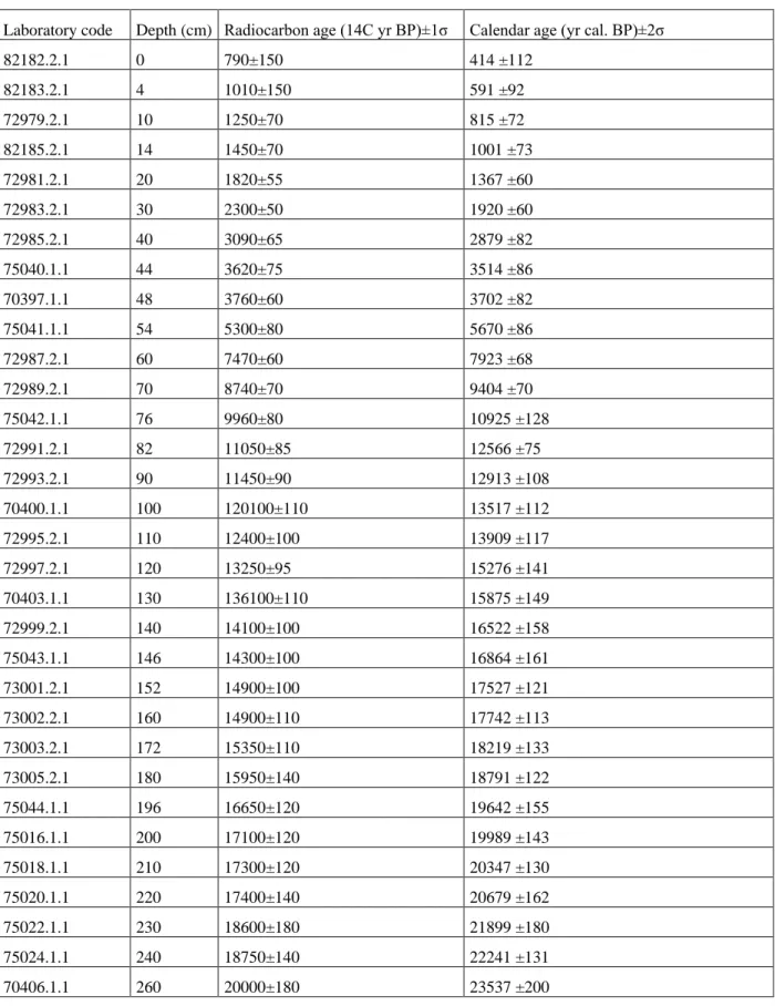
Laboratory code Depth (cm) Radiocarbon age (14C yr BP)±1σ Calendar age (yr cal. BP)±2σ
82182.2.1 0 790±150 414 ±112 82183.2.1 4 1010±150 591 ±92 72979.2.1 10 1250±70 815 ±72 82185.2.1 14 1450±70 1001 ±73 72981.2.1 20 1820±55 1367 ±60 72983.2.1 30 2300±50 1920 ±60 72985.2.1 40 3090±65 2879 ±82 75040.1.1 44 3620±75 3514 ±86 70397.1.1 48 3760±60 3702 ±82 75041.1.1 54 5300±80 5670 ±86 72987.2.1 60 7470±60 7923 ±68 72989.2.1 70 8740±70 9404 ±70 75042.1.1 76 9960±80 10925 ±128 72991.2.1 82 11050±85 12566 ±75 72993.2.1 90 11450±90 12913 ±108 70400.1.1 100 120100±110 13517 ±112 72995.2.1 110 12400±100 13909 ±117 72997.2.1 120 13250±95 15276 ±141 70403.1.1 130 136100±110 15875 ±149 72999.2.1 140 14100±100 16522 ±158 75043.1.1 146 14300±100 16864 ±161 73001.2.1 152 14900±100 17527 ±121 73002.2.1 160 14900±110 17742 ±113 73003.2.1 172 15350±110 18219 ±133 73005.2.1 180 15950±140 18791 ±122 75044.1.1 196 16650±120 19642 ±155 75016.1.1 200 17100±120 19989 ±143 75018.1.1 210 17300±120 20347 ±130 75020.1.1 220 17400±140 20679 ±162 75022.1.1 230 18600±180 21899 ±180 75024.1.1 240 18750±140 22241 ±131 70406.1.1 260 20000±180 23537 ±200
Table 1. Age model for core SHAK06–5K, based on monospecific samples of the planktonic 675
foraminifera Globigerina bulloides. Convention radiocarbon ages and associated 1σ uncertainties 676
have been rounded according to convention. 677 678 679 680 681 682 683 684 685 686 687 688 689 690 691 692 693 694 695 696 697 698 699 700 701 702 75028.1.1 270 20400±150 24012 ±156 75030.1.1 280 20700±150 24482 ±179 75048.1.1 284 201000±160 24781 ±215 75032.1.1 290 21300±160 25245 ±186 75033.1.1 300 22100±170 25936 ±125 75034.1.1 310 22600±180 26416 ±184 75036.1.1 320 23000±180 26974 ±210 75038.1.1 329 24100±200 27800 ±163
703 704 705 706
Table 2. Influence of the sample preparation method on radiocarbon ages. 14C ages and 707
associated 1-σ confidence level (68.2% probability), and corresponding age discrepancies, shown 708
in figure 2. Age offsets that can be explained within the 1-σ confidence level of the associated 709
dates are indicated in bold. 710
G. bulloides from non-extracted sediments G. bulloides from sediments extracted with organic
solvents
G. bulloides- G. bulloides
Leached sample Leachate
Leached sample- Leachate
Leached sample Leachate
Leached sample-Leach fraction Leached Sample (Extracted sediment)-Leached sample (non-extracted sediment) Depth (cm) Lab code ETH- 14C age (yr)± 1 σ Lab code ETH- 14C age (yr)± 1 σ Age difference (yr) Lab code ETH- 14C age (yr)±1 σ Lab code ETH- 14C age (yr)± 1 σ Age difference (yr) Age difference (yr) 120 90559. 1.1 12901±86 90559 .2.1 12846±135 55±160 72997. 2.1 13228±93 72997 .1.1 12328±190 900±211 327±126 172 90557. 1.1 15262±100 90557 .2.1 13377±134 1885±167 73003. 2.1 15346±115 73003 .1.1 13730±202 1616±232 84±152 210 90555. 1.1 17303±109 90555 .2.1 16651±167 652±199 75018. 1.1 17292±123 75018 .2.1 15468±242 1824±271 -11±164 240 90553. 1.1 18529±119 90553 .2.1 16378±162 2151±201 75024. 1.1 18735±134 75024 .2.1 16214±256 2521±288 206±179 300 90552. 1.1 22171±152 90552 .2.1 21509±237 662±281 75033. 1.1 22110±172 75033 .2.1 20832±342 1278±382 -61±229 711 712
Table 3. Radiocarbon ages and associated 1-σ confidence level (68.2% probability), and 713
corresponding age discrepancies. * Stands for untreated samples. Numbers in bold indicate age 714
offsets that can be explained within the 1-σ confidence level of the associated dates. 715 G. bulloides G. ruber G. bulloides- G. ruber G. bulloides- G. bulloides
Leached sample Leachate
Leached sample- Leachate
Leached sample Leachate
Leached sample-Leach fraction Leached sample-Leached sample Leached sample-Untreated sample Depth (cm) Lab code ETH-14C age (yr)± 1 σ Lab code ETH-14C age (yr)± 1 σ Age difference (yr) Lab code ETH-14C age (yr)±1 σ Lab code ETH-14C age (yr)± 1 σ Age difference (yr) Age difference (yr) Age difference (yr) 0 *82182. 2.1 788±151 4 *82183. 2.1 1012±153 10 82184.2 .1 1253±71 82184. 1.1 1373±77 120±105 72980.2 .1 1463±45 72980. 1.1 1216±108 247±117 -210±84
*72979. 1.1 1458±110 -205±131 14 *82185. 2.1 1451±70 20 72981.2 .1 1820±55 72981. 1.1 2078±124 -258±136 72982.2 .1 1884±46 72982. 1.1 1930±113 -46±122 -64±72 30 72983.2 .1 2301±47 72983. 1.1 2229±120 72±129 72984.2 .1 2471±75 72984. 1.1 2349±123 122±144 -170±88 40 72985.2 .1 3087±64 72985. 1.1 2927±117 160±133 *72986. 1.1 2628±185 44 75040.1 .1 3619±74 75040. 2.1 3823±124 -204±144 48 70397.1 .1 3762±62 70397. 2.1 3848±122 -86±137 70399.1 .1 3389±63 70399. 2.1 3137±123 252±138 373±88 54 75041.1 .1 5295±80 75041. 2.1 5343±122 -48±146 60 72987.2 .1 7470±63 72987. 1.1 6556±149 914±162 72988.2 .1 6705±60 72988. 1.1 6964±207 -259±215 765±87 220±90 *90560. 1.1 7250±64 70 72989.2 .1 8744±69 72989. 1.1 8731±156 13±171 72990.2 .1 8482±89 72990. 1.1 8261±157 221±180 262±113 76 75042.1 .1 9957±76 75042. 2.1 9338±160 619±177 82 72991.2 .1 11056±84 72991. 1.1 10351±180 706±199 72992.2 .1 10204±75 72992. 1.1 10130±175 74±190 852±113 90 72993.2 .1 11437±86 72993. 1.1 11191±178 246±198 72994.2 .1 10806±104 72994. 1.1 10854±174 -48±203 631±135 100 70400.1 .1 12077±107 70400. 2.1 11261±193 816±221 70402.1 .1 11900±105 70402. 2.1 11442±201 458±227 177±150 110 72995.2 .1 12385±103 72995. 1.1 12413±187 -28±213 *72996. 1.1 12318±210 120 72997.2 .1 13228±93 72997. 1.1 12328±190 900±211 72998.2 .1 12198±91 72998. 1.1 12688±198 -490±218 1030±130 130 70403.1 .1 13615±109 70403. 2.1 12794±204 821±231 70405.1 .1 13193±109 70405. 2.1 12905±304 288±323 422±154 336±140 *90558. 1.1 13279±88 140 72999.2 .1 14090±104 72999. 1.1 13535±199 555±224 73000.2 .1 13252±596 73000. 1.1 11980±272 1272±655 838±605 146 75043.1 .1 14290±101 75043. 2.1 13079±225 1211±247 152 73001.2 .1 14884±105 73001. 1.1 14160±216 724±240 160 73002.2 .1 14924±108 73002. 1.1 14334±210 590±236 172 73003.2 .1 15346±115 73003. 1.1 13730±202 1616±232 *73004. 1.1 14572±328 191±154 *90556. 1.1 15155±102 180 73005.2 .1 15977±138 73005. 1.1 14560±207 1417±249 73006.2 .1 15261±230 73006. 1.1 15071±339 190±410 716±268 190 73007.2 .1 15916±206 73007. 1.1 16179±247 -263±322 *73008. 1.1 15513±260 196 75044.1 .1 16636±120 75044. 2.1 15351±270 1285±295 200 75016.1 .1 17066±120 75016. 2.1 16105±238 961±266 75017.1 .1 16786±134 75017. 2.1 16599±267 187±299 280±180 210 75018.1 .1 17292±123 75018. 2.1 15468±242 1824±271 *75019. 1.1 17064±161 214 75045.1 .1 17242±122 75045. 2.1 16159±279 1083±304
220 75020.1 .1 17427±142 75020. 2.1 16248±270 1179±305 75021.1 .1 17511±137 75021. 2.1 16493±260 1018±294 -84±197 230 75022.1 .1 18634±176 75022. 2.1 17495±259 1139±313 *75023. 1.1 18146±170 234 75046.1 .1 18305±130 75046. 2.1 17318±278 987±307 240 75024.1 .1 18735±134 75024. 2.1 16214±256 2521±289 75025.1 .1 18301±177 75025. 2.1 17803±280 498±331 435±222 1154±182 *90554. 1.1 17581±123 250 75026.1 .1 18726±150 75026. 2.1 18314±288 412±325 75027.1 .1 19231±141 75027. 2.1 18481±289 750±322 -506±206 260 70406.1 .1 19979±181 70406. 2.1 18387±301 1592±351 70408.1 .1 19831±180 70408. 2.1 18166±307 1665±356 148±255 264 75047.1 .1 19776±143 75047. 2.1 17717±276 2059±311 270 75028.1 .1 20361±152 75028. 2.1 17665±287 2696±325 *75029. 1.1 18348 ±172 270 r *82186. 2.1 18310±320 280 75030.1 .1 20684±155 75030. 2.1 17045±257 3639±300 *75031. 1.1 15814±166 284 75048.1 .1 20991±159 75048. 2.1 18691±319 2300±356 290 75032.1 .1 213487±161 75032. 2.1 20247±338 1100±374 300 75033.1 .1 22110±172 75033. 2.1 20832±342 1278±383 310 75034.1 .1 22573±178 75034. 2.1 20153±339 2420±383 *75035. 1.1 21912±278 314 75049.1 .1 23133±189 75049. 2.1 21020±484 2113±519 320 75036.1 .1 22984±185 75036. 2.1 19376±305 3608±357 *75037. 1.1 22763±286 1419±242 *90551. 1.1 21565±157 329 75038.1 .1 24126±203 75038. 2.1 20116±317 4010±376 *75039. 1.1 23166±329 716 717 718 719 720