An integrated approach for the measurement of inequality, poverty, and richness

(1)

PANOECONOMICUS, 2015, Vol. 62, Issue 5, pp. 531-555

Received: 21 October 2012; Accepted: 17 May 2015.

UDC 330.564:330.59] (469) DOI: 10.2298/PAN1505531C Original scientific paper

Nuno Crespo

Business School Economics Department,

Lisbon University Institute (ISCTE-IUL); ISCTE-IUL,

Business Research Unit, Portugal

 [email protected]

Sandrina B. Moreira

Department of Economics and Management,

Polytechnic Institute of Setúbal; ISCTE-IUL,

Business Research Unit, Portugal

 [email protected] Nadia Simoes

ISCTE-IUL, Business School Economics Department; ISCTE-IUL, Business Research Unit, Portugal

 [email protected]

Acknowledgement: We are grateful to

the Office of National Statistics (INE) for kindly providing us with the survey data, and we acknowledge the financial support from Fundação para a Ciência e para a Tecnologia

(PEst-OE/EGE/UI0315/2011). The usual disclaimer applies.

An Integrated Approach for the

Measurement of Inequality,

Poverty, and Richness

Summary: The goal of the paper is to propose a new and integrated approach

to the measurement of inequality in income distribution, poverty, and richness. The proposed set of indicators is easy to calculate and is based on a neutral inequality concept. The method allows an objective interpretation of the values for each measure, a decomposition according to households’ characteristics, and an immediate comparison of the results between countries and time pe-riods, thereby offering important conclusions for policy action. We illustrate the application of the measures with data from Portugal, finding that: (i) 17.78% of the individuals belong to households classified as poor while 7.03% are rich and 75.19% are classified as middle class; (ii) it is necessary to redistribute 23.78% of the total income of the economy to obtain perfect equality; (iii) 2.09% of the total income in the economy is enough to eradicate poverty.

Key words: Income inequality, Poverty, Richness, Measurement. JEL: D30, D31.

Income inequality and poverty are well established research fields in the economic literature. Apart from a multiplicity of other empirical and theoretical contributions, several recent books address the state of the art of the research about inequality and poverty, including Frank A. Cowell (2011) and Wiemer Salverda, Brian Nolan, and Timothy M. Smeeding (2011). This analysis can be justified on several grounds. On the one hand is the natural wish to address an issue seen as socially unfair. On the other hand, economic policy concerns have brought the issue of poverty and inequal-ity to the center of public debate, intensifying the research into their determinants. A full knowledge of the real dimension and characterization of these phenomena is thus of widespread interest, seeking the definition of effective socio-economic policies (Anthony B. Atkinson 2015).

From a methodological point of view, several measures are commonly used to assess the quantitative importance of these phenomena. In the specific case of pov-erty, three dimensions are considered, covering different perspectives of this topic, namely its incidence, intensity and severity.

(2)

532 Nuno Crespo, Sandrina B. Moreira and Nadia Simoes

Three reasons justify the analysis of the “rich”: their command over resources, their command over people (income and wealth as sources of power) and their global significance (Atkinson 2007). Central to all this literature has been the discussion of the procedures and indicators for measuring income inequality, poverty, and rich-ness. The present paper contributes to this line of research by proposing a new meth-odology that allows an integrated approach for measuring inequality, poverty, and richness. This is accomplished through the consideration of a common conceptual framework that allows the derivation of a range of measures to quantify different dimensions of these phenomena.

Our approach starts from an inequality measure that is based on a concept of inequality characterized by its neutrality, seeking to quantify the phenomenon with-out value judgments on the distribution of inequality. The approach has the following characteristics: (1) simplicity in application; (2) an objective interpretation of the values obtained for each indicator; (3) a straightforward comparison of the results between different economic spaces and time periods; (4) decomposability (i.e. the possibility of knowing the contribution of population’s sub-groups).

The paper is structured as follows. Section 1 summarizes the main methodo-logical issues and indicators used in the literature. Section 2 presents the approach in which new measures of inequality, poverty, and richness are advanced. Section 3 illustrates the application of the proposed measures using data for Portugal. Section 4 presents some final remarks.

1. Methodological Issues and Indicators

For the empirical analysis of inequality, poverty, and richness, it is necessary to as-sume some methodological choices as well as to select the indicator(s) that will be used. In this section, we summarize the main options available.

1.1 Methodological Issues

Measuring income inequality, poverty, and richness implies making choices concern-ing some methodological issues. Four of these issues are common to the analysis of the three phenomena while a fifth is specific to the analysis of poverty and richness. The first group involves choices concerning: (a) the indicator of resources; (b) the demographic unit; (c) equivalence scales; (d) the weighting of the demographic unit. In order to measure poverty / richness, it is also necessary to define a poverty / rich-ness line.

In relation to the indicator of resources, Cowell (2011) suggests that wealth, lifetime income, and income are in that order the most adequate ones, even though none of them covers completely the command over resources for all goods and ser-vices in society. The ease of calculation and, mainly, data availability usually justify income as the favored option. Regarding the concept of income, the most common option - given the availability of statistical information - is the monetary disposable income. This choice is subject to criticism because of the exclusion of non-monetary forms of income and also of the past accumulation effect through savings and indeb-tedness.

(3)

533 An Integrated Approach for the Measurement of Inequality, Poverty, and Richness

The second methodological choice relates to the demographic unit, usually be-tween the individual and an aggregate (family or household, the latter also including individuals at the same address who are not part of the nuclear family). The option for households is mainly followed in the literature because of the income sharing phenomenon within the household.

Directly related to the previous option is the issue of comparing unlike units. Households with different compositions and dimensions have different needs and thus require different levels of income to achieve similar levels of well-being. The use of equivalence scales allows calculating equivalent adults for each household. A frequently used equivalence scale is the OECD modified scale, which gives a weight of 1 to the first adult, 0.5 to each of the remaining adults, and 0.3 for children under 14 years of age. The income adjusted by the composition and dimension of the household - the adult equivalent income - represents therefore a refinement of the income per capita, not neglecting the existence of economies of scale due to the share of housing and expenses. Disregarding inequality within the household is the main limitation of this concept. Therefore, it implies the under-estimation of the ac-tual degree of inequality existing in society.

Concerning the weighting of the demographic unit, the usual choice is to take the number of a household’s individuals.

The fifth methodological issue - the poverty / richness line - is exclusive to the analysis of poverty and richness. The main methodological question in this context is the choice between absolute or relative lines. In the first case the threshold is defined without reference to the standard of living prevailing in society. In the second case that reference is taken into account.

1.2 Indicators

1.2.1 Inequality Indicators

Four main groups of inequality indicators can be considered. The first refers to measures that compare the income share of the top x% of the income distribution with that of the bottom x%. Frequent values for x are 5, 10, and 20. The main advan-tage of this type of indicator is the ease of calculation and interpretation. However, evaluating inequality through these measures is limited because the income distribu-tion inside each income group is not considered (Jonathan Haughton and Shahidur R. Khandker 2009).

The most widely used measure of income inequality is the well-known Gini coefficient, which varies between 0 (total equality) and 1 (maximum inequality). However, this index is not (easily) decomposable.

A third way to measure inequality is the Atkinson index. Its most important characteristic is making the value judgments involved in the measurement of inequa-lity explicit, by taking into account a parameter that captures the degree of inequainequa-lity aversion. That parameter can vary between 0 (inequality indifference) and + (cor-responding to the Rawlsian criterion that values only the income of the poorest).

A last group of inequality indicators corresponds to the Generalized entropy (GE) measures, including the Theil indices and the mean log deviation measure

(4)

(Cowell and Kiyoshi Kuga 1981a, b). Similar to the Atkinson index, GE measures clearly assume the incorporated value judgments through a parameter representing the weight attributed to income differences in different parts of the distribution. The most common values for that parameter are 0, 1, and 2. The inexistence of inequality implies that GE measures assume a value of 0. The increase of the value of such in-dicators corresponds to an increase in inequality.

1.2.2 Poverty Indicators

Several poverty measures are available in the literature, capturing the different di-mensions of this phenomenon (incidence, intensity, and severity). The headcount index (P0) captures the first dimension, measuring the proportion of individuals

clas-sified as poor (i.e. with an income lower than the poverty line) in the total population. An important weakness of P0 is the fact that it is only an accounting of the poor, with

no sensibility regarding the magnitude of the problem.

In its turn, the poverty gap index (P1) measures the mean deviation of income

from the poverty line, capturing the intensity of poverty. Thus P1 overcomes the

main limitation of P0.

The poverty severity index (P2) is a third poverty indicator, which measures

the inequality among the poor by calculating the sum of poverty gaps weighted by the gaps themselves (Haughton and Khandker 2009). Thus, P2 is especially affected

by extreme poverty situations.

A particularly appealing way to present the three above measures of poverty is through the class of poverty measures proposed by James Foster, Joel Greer, and Erik Thorbecke (1984): , 1 N Z i G P N i















    (1)

in which N is the total number of individuals in the population, Z the poverty line, and Gi the poverty gap associated with individual i. Gi will be zero if the income of i

(Yi) is greater than or equal to Z and (Z - Yi) in the opposite case (i.e. when i is poor).

The parameter  (  0) represents the sensitivity of the index to poverty. When  is 0, 1, and 2, one obtains the poverty measures mentioned above, that is, the headcount index, the poverty gap index, and the poverty severity index, respectively. Decompo-sability is an interesting property of Pα.

1.2.3 Richness Indicators

The analysis of top incomes has emerged in the last decade and is today a well-established field of literature (Thomas Piketty 2005; Piketty and Emmanuel Saez 2006; Jesper Roine and Daniel Waldenström 2008; Atkinson and Piketty 2010; Fa-cundo Alvaredo et al. 2013; Atkinson and Andrew Leigh 2013). There is a more re-cent research line that looks into the distribution of income and wealth using a

(5)

dy-535 An Integrated Approach for the Measurement of Inequality, Poverty, and Richness

namic approach seeking to assess how the share of top wealth / income decile in total wealth / income has evolved over a long period of time and to identify the causes for the observed patterns by focusing and comparing the role of national institutions and historical circumstances (for the most important contribution in this area see Piketty 2014; for other contributions see also Piketty and Saez 2014; Saez and Gabriel Zuc-man 2014).

While the methodologies used to analyze inequality and poverty are well con-solidated in the literature, this is not so for the evaluation of richness (Andreas Peichl, Thilo Schaefer, and Christoph Scheicher 2010). In that context, the most commonly applied measures are the income share of the top x% of the income distri-bution and headcount measures. As stated above, both measures have serious limita-tions however, and thus give only a partial indication of the richness phenomenon. An important contribution is given by Peichl, Schaefer, and Scheicher (2010), who have suggested a class of richness measures analogous to those existing for the po-verty measures.

2. An Integrated Approach for the Measurement of Inequality,

Poverty, and Richness

2.1 On the Concept(s) of Income Inequality

In the previous section we synthesized the most common methodological options for the measurement of inequality, poverty, and richness, as well as the main indicators available, stressing their specificities and (implicit or explicit) value judgments.

In this section we propose a new and integrated approach for measuring these phenomena. We start by considering a new measure of income inequality. Consider-ing a common conceptual framework, we then derive poverty and richness measures, capturing their different dimensions (incidence, intensity, and severity).

However, “before trying to quantify anything one must first be clear about the concept to be measured” (Martin Ravallion 2003, p. 740). We therefore start the analysis by discussing the concept of inequality underlying the indicator that serves as our point of departure.

As argued by Lorenzo G. Bellù and Paolo Liberati (2006, p. 2), “inequality is not a self-defining concept, as its definition may depend on economic interpretations as well as ideological and intellectual positions”. Although an explicit discussion about the different concepts of inequality underlying the measures available does not exist in the literature, one can distinguish four main concepts.

A first - the simplest - associates inequality with the difference, in absolute terms, between the current distribution and the egalitarian one (concept of inequality 1). The second and third concepts of inequality are relative measures of inequality. While the first one - concept of inequality 2 - measures the deviation from the benchmark distribution in relative terms, the concept of inequality 3 also takes into account the distribution of inequality among the different receiving units. The last concept - concept of inequality 4 - explicitly incorporates welfare considerations in the measurement of inequality (e.g. Amartya Sen 1976), arguing that the level of in-come should also be considered in the assessment of this phenomenon. A distribution

(6)

B obtained from a distribution A by doubling all incomes, corresponds to a better situation since it ensures a higher level of welfare.

This conceptual discussion is critical because the inequality indices used for empirical purposes should reflect the specific concept considered. The measures that correspond to each of the concepts presented above can be distinguished by their compliance with the principles proposed by Gary Fields and John C. H. Fei (1978), which are usually applied in the analysis of inequality indicators, namely: (i) symme-try; (ii) population size independence; (iii) mean independence; (iv) Pigou-Dalton transfers principle.

The principle of symmetry requires that any measure of inequality should be invariant to swaps of income among individuals. According to the principle of popu-lation size independence, the inequality measure should not change in response to a replication of the original population. The principle of mean independence requires that the index must not vary when all the original incomes are multiplied by a con-stant. Finally, according to the Pigou-Dalton transfers principle, any transfer of in-come from a richer to a poorer individual that does not reverse their positions, reduc-es inequality.

Table 1 synthesizes the principles verified by the measures included in each of the four concepts of inequality.

Table 1 Inequality Concepts and the Principles Proposed by Fields and Fei (1978) Principles

Symmetry Population size _independence _independenceMean _{transfers principle}Pigou-Dalton

Concept 1 Yes Yes No No

Concept 2 Yes Yes Yes No

Concept 3 Yes Yes Yes Yes

Concept 4 Yes Yes No Yes

Source: Own elaboration. Given the notable differences between the various concepts of inequality it is important: (1) to discuss which ones seem more appropriate for a proper measure-ment of the phenomenon; (2) to justify the option assumed in the present study.

In the context of concept 1, a distribution B derived from a distribution A by multiplying all incomes by a positive constant reveals a greater degree of inequality than the original distribution. This breach of the mean independence principle makes this concept difficult to accept as an adequate basis for empirical measures of inequa-lity.

According to the concept of inequality 4, the comparison of distributions A and B leads to the opposite conclusion. In this case, B is preferable because it pro-vides a higher level of welfare. This concept is subject to criticism, however, because it captures more than what the concept of inequality is intended to measure.

In this study we argue that the indicators that fulfil the proprieties of the con-cepts of inequality 2 and 3 are the most interesting for measuring inequality. It is

(7)

im-537 An Integrated Approach for the Measurement of Inequality, Poverty, and Richness

portant to note, however, that these concepts capture different perspectives of the phenomenon and should therefore not be seen as alternatives, but rather as comple-ments.

Concept 3 is the framework of the inequality measures most frequently used in the literature, such as those generally discussed in Section 1. Indicators that belong to this concept assume the simultaneous verification of the four principles suggested by Fields and Fei (1978). The Pigou-Dalton principle is not, however, immune to criti-cism, as noted, for example, by Alain Chateauneuf and Patrick Moyes (2006) in a study entitled “measuring inequality without the Pigou-Dalton condition”. Discuss-ing the inclusion of this principle in most measures of inequality, the authors argue that “one may however raise doubts about the ability of such a condition to capture the very idea of inequality in general” (Chateauneuf and Moyes 2006, p. 2). Further discussion on this issue is provided by Brice Magdalou and Moyes (2009) and Mag-dalou and Richard Nock (2011). Some experimental studies also confirm that the principle of transfers is not universally accepted, as shown, for instance, by Yoram Amiel and Cowell (1992) and Wulf Gaertner and Ceema Namezie (2003).

Based on these considerations, in this study we assume the concept of inequa-lity 2. As a result, our inequainequa-lity index does not verify the Pigou-Dalton principle. The reason for this choice stems directly from the main distinguishing feature of this concept in comparison to concept 3 - its neutrality (i.e. the exclusion of any kind of distribution sensitivity). The measures based on this concept seek only the quantifica-tion of the phenomenon. Following this perspective, the measure that we suggest below aims to quantify the distance between the current distribution and the egalita-rian one, without any value judgment on the distribution of inequality. This index measures the proportion of the total income that would be necessary to redistribute in order to obtain equality.

In addition to the neutrality that characterizes the measure of inequality and the full range of indicators of poverty and richness derived from it, the approach de-veloped throughout this section has other appealing features: (a) it is an integrated perspective of inequality, poverty, and richness; (b) the simplicity of calculation of the suggested indicators; (c) their decomposability, allowing the identification of the contribution of population’s sub-groups; (d) the specific economic interpretation of the values obtained, as opposed to most available measures, whose values can only be interpreted by comparison with figures for other countries or periods. The latter is an important feature to the extent that the several indices provide useful information for the definition of policy interventions.

Regarding the methodological questions presented in the previous section, we assume the most common choices concerning the second and third issues - house-holds as recipient units of income and an equivalence scale (namely the OECD mod-ified scale) to account for the existence of economies of scale - while following a different approach in relation to the fourth and fifth questions previously mentioned. The first option is unnecessary for the present section. We will return to that subject in Section 3.

(8)

2.2 Income Inequality

Taking into account the discussion of the previous section, our inequality index (I) is defined as: , 1



   N i i i I    (2) in which: , 1



  _N i i i i Y Y  (3) and . 1



  _N i i i i D D



(4)

N is the total number of households, Yi represents the total income of

house-hold i, and Di expresses the number of equivalent adults in that household. Thus, i

is the weight of household i in the total income of the society and _i_{its weight in}

terms of dimension (evaluated through the concept of equivalent adults). There will be an equality situation in the income distribution when all households have an in-come share equal to their share in terms of equivalent adults, that is, when

i i

i    , _.

When we set  = 0.5, the possible values for I are in the range [0, 1. The val-ue 0 is obtained when all the households have a share of the total income of the economy equal to their share in terms of dimension (evaluated through equivalent adults). The other extreme case, leading I to converge to 1, occurs when the full amount of income in the society belongs to a very small household. It should be noted that the admissible range is open at right because the value of 1 corresponds to a situation where the full amount of income is held by households of a zero dimen-sion, an impossible case since we cannot have households of zero dimension. Setting

 = 0.5 allows a more intuitive interpretation of the results - which is its only purpose - being therefore more adequate than alternatives such as  = 1, according to which I would vary between 0 and 2.

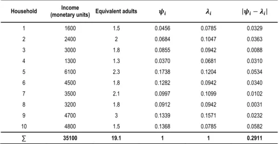
In order to illustrate the main point of our inequality measure, let us consider a very simple example by assuming a society composed of only ten households, with the incomes and equivalent adults presented in Table 2.

Considering this simple example, we obtain I = 0.1456 (in the range [0, 1 where 0 means perfect equality and 1 maximum inequality).

(9)

Table 2 An Illustrative Example

Household _{(monetary units)}Income Equivalent adults | − |

1 1600 1.5 0.0456 0.0785 0.0329 2 2400 2 0.0684 0.1047 0.0363 3 3000 1.8 0.0855 0.0942 0.0088 4 1300 1.3 0.0370 0.0681 0.0310 5 6100 2.3 0.1738 0.1204 0.0534 6 4500 1.8 0.1282 0.0942 0.0340 7 3500 2.1 0.0997 0.1099 0.0102 8 3200 1.8 0.0912 0.0942 0.0031 9 4700 3 0.1339 0.1571 0.0232 10 4800 1.5 0.1368 0.0785 0.0582 ∑ 35100 19.1 1 1 0.2911

Source: Own elaboration. Taking into account the inequality measure, I, we can now deepen the analy-sis, proposing poverty and richness measures. The first step is to set criteria to define if household i is poor (P), rich (R), or if it is in an intermediate situation, which we will call middle class (MC). These criteria are based on the comparison between what the household has in terms of income with what it should have, considering its di-mension and composition, in order to obtain an equal distribution of resources:

, 1 if 1 if if i i i i i i                           P MC R S_i (5) in which , _{≥ 1.}

A specific household i will be classified as rich when the share that it holds in terms of income is significantly higher than its share in terms of dimension. As pre-sented in Equation (5), this is the case when > ⇔ > , with ≥ 1. For each empirical application, the researcher needs to define the value of the parameter . Higher values for reduce the range in which the household is classified as rich and amplifies the middle class range.

A similar reason is valid for the definition of the poor. In this case, a house-hold will be classified as poor if its share in terms of income is significantly lower

(10)

than its share in terms of dimension. This occurs when > . This corresponds, as presented in Equation (5), to < with ≥ 1.

Once we classify each household according to its position in the income dis-tribution, we can obtain aggregated measures of poverty and richness.

2.3 Poverty

As seen above, a detailed analysis of poverty should take into account three dimen-sions: incidence, intensity, and severity. Following the approach presented in the previous section, we now propose poverty measures that focus on each of these di-mensions. Additionally, we discuss the case of the near-poor.

We start by defining a measure of poverty incidence (POV). Defining Hi as the

number of individuals of household i, then:

. 1 ) ( 1



    _N i i N P Si i H H POV i (6)

POV is a headcount index, indicating the percentage of individuals that belong to poor households in relation to the total number of individuals.

Following, we define an index of poverty intensity (POVʹ). Let us start by cal-culating . If household i is classified as poor then < ⇔ − > 0. ex-presses the percentage of the total income in the economy that household i would have to receive to become non-poor:

.

i i i _ 

   (7)

Summing up for all the poor households, we obtain POVʹ. This measure cor-responds to the percentage of the total income in the economy that needs to be trans-ferred from the non-poor to the poor in order to eradicate poverty:

. ' 1



   N P Si i i POV  ₍₈₎

If we divide POVʹ by the number of poor households, we obtain an indicator of the average intensity of poverty.

The third dimension of poverty that needs to be taken into account is its sever-ity. To capture this dimension, we consider a set of indicators that aim to reflect dif-ferent aspects of the phenomenon. For this the first step of our analysis is the defini-tion of a new poverty threshold reflecting a higher degree of resource privadefini-tion. Therefore, a situation of extreme poverty is defined as:

(11)

, 1 if    _  i i i SP S (9)

in which

ζ

> 1. By multiplying by

ζ

(with

ζ

> 1), we define (see the discussion above) that a household i is classified as extremely poor when the difference between the share of that household in the total economy in terms of dimension and its share in terms of income is higher than in the case of poverty.

With reference to this line of extreme poverty, we can quantify the incidence and intensity of severe poverty. The incidence of severe poverty is defined as in the case of POV (Equation (6)) but considering now the households classified as ex-tremely poor. It can be defined in relation to either the total population or the poor population, being expressed, respectively, as follows:



     _N i i N SP Si i H H POV S i 1 ) ( 1 ) 1 ( (10) and . ) 2 ( ) ( 1 ) ( 1



     _N P Si i N SP Si i i i H H POV S (11)

In a similar vein, the intensity of severe poverty can be calculated by reference to either the poverty line or the severe poverty line, being measured, respectively, as:









N SP Si i i

POV

S

) ( 1

)

1 (

'



₍₁₂₎ and

,

)

2 (

'

) ( 1



 





N SP Si i i

POV

S



₍₁₃₎

in which corresponds to its expression in (7) and:

.

i i i

_











(14)

(12)

The measures of severe poverty intensity express the percentage of the total income in the economy that would be necessary to transfer to the extremely poor in order to take them out of poverty (in the case of S-POVʹ(1)) or severe poverty (in the case of S-POVʹ(2)).

To complement the analysis of the severity of poverty, we adopt an alternative perspective, following the method most commonly applied in the literature. To that end, we calculate an inequality index among poor (IP):

,

) ( 1



 





N P Si i i P i

k

I





₍₁₅₎ in which: , ) ( 1



   _N P Si i i i i Y Y



(16) and . ) ( 1



   _N P Si i i i i D D



(17)

This inequality index among the poor (IP) is defined following the same basic

principle as our baseline measure of inequality (I), meaning that we are comparing the share of each household i in the total of the economy in terms of income and in terms of dimension. The only difference is the fact that in the case of we are re-stricting the analysis to the households previously classified as poor (Si = P) while I

considers all the households.

As , the most obvious value for the parameter k is 0.5. In that case our meas-ure of inequality among the poor will range between 0 and 1.

This indicator quantifies the percentage of the total income of poor households that has to be redistributed among them in order to obtain an equal intensity of pover-ty. An increase in IP reflects higher levels of poverty severity.

Finally, let us consider the case of the near-poor. An effective poverty policy cannot focus only on the poor, but should, in line with the analysis of poverty vulne-rability (Lant Pritchett, Asep Suryahadi, and Sudarno Sumarto 2000; Ricardo Gui-marães 2007; Indranil Dutta, Foster, and Ajit Mishra 2011; Martina Celidoni 2013; Nancy Birdsall, Nora C. Lustig, and Christian J. Meyer 2014), also give special at-tention to those who are very near to being poor in order to avoid new poverty cases. Accordingly, we propose measures to capture the importance of this phenomenon. Defining Si = P+ as meaning near-poverty, we have:

(13)

,

1 if















 i i i

P

S

(18) in which 11  .

Near-poverty incidence, representing the percentage of individuals that belong to near-poor households in relation to total population, is given by:

. 1 1



   _  N i i N ) P (S i i H H POV i (19)

In this context, it is also interesting to know the safety net of the near-poor population. For household i, that safety margin is given by the symmetric of i. In

overall terms, we quantify this as:

, ) ( ) ( 1 ) ( 1

'



  _   _ _         N P S i i N P S i i i i i

POV

    ₍₂₀₎

expressing the percentage of the total income in the economy by which the near-poor are above the poverty line. The average safety margin of near-poor can be obtained by dividing POVʹ+ by the number of near-poor households.

2.4 Other Dimensions

The indicators used in the analysis of poverty can be adapted for the measurement of the corresponding richness dimensions. We thus conceive incidence, intensity, and severity measures of richness (on the definition of the richness line, see Marcelo Me-deiros 2006). For terminological reasons, we opt to designate the last case as “rich-ness depth”.

Additionally, we consider that, although less explored, the topic of inequality in the middle class is also an important dimension of analysis, capturing the degree of countries’ economic and social cohesion. For a discussion on the quantitative lim-its and socio-economic characteristics of this income group see, for instance, Atkin-son and Andrea Brandolini (2011).

In the Appendix, we present the measures of richness and middle class inequa-lity.

(14)

3. Inequality, Poverty, and Richness - An Application with

Evidence from Portugal

3.1 Data and Empirical Evidence

In order to illustrate the application of the set of measures presented in the previous section, we consider data from Portugal, since it is among the European countries with the highest levels of inequality and poverty. According to the European Union Statistics on Income and Living Conditions (EU-SILC), in 2013, Portugal was the fifth country in the EU-28 with the highest level of inequality and the fourth country in the EU-15 with the highest level of poverty (9th position considering the EU-28).

We use micro-data on the income and structure of households living in Por-tugal from the Office of National Statistics (INE)’s Household Budget Survey (IDEF) of 2005/2006. The results are based on a representative sample of the Portu-guese economy with 10,403 households and a total of 28,359 individuals. The IDEF is a large-dimension survey associated with a questionnaire filled in by households with detailed information on the whole set of collective and individual expenditures. It also includes demographic data, income data, and data on non-frequently con-sumed goods and services.

The subsequent analysis takes into account not only monetary income but also total income. The comparison of the results is particularly important for two reasons: (i) the relative weight of non-monetary income (approximately 19% of total income); (ii) the asymmetry in the non-monetary income distribution. In the case of total in-come, the following items are also considered: the value of goods produced for own consumption, inputted rents, and remuneration in kind. Alari Paulus, Holly Suther-land, and Panos Tsakloglou (2010) provide a discussion on the importance of non-monetary income.

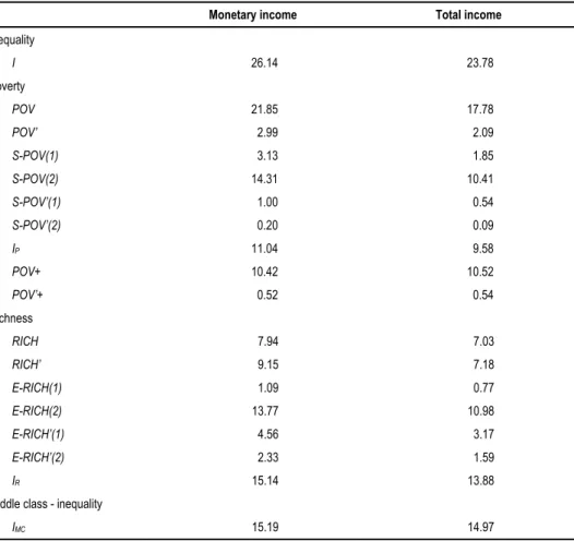
Table 3 presents the results of the application of the proposed indicators taking as a reference the following values for the parameters:  = 0.5,  = 2,  = 2,  = 2,

 = 0.5,  = 0.6,  = 2,  = 0.5, and  = 0.5.

Focusing on the results based on total income, we find the need to redistribute 23.78% of the total income in the economy to reach a situation of equality in income distribution. It is important to note, however, that such an overall value presupposes an adequate redistribution of income, that is, one that does not waste resources.

Regarding the distribution of individuals by income groups, we conclude that 17.78% are poor, 7.03% are rich, and the remaining 75.19% are from the middle class. Concentrating on the bottom of the income distribution, we see that 10.41% of the poor (corresponding to 1.85% of the total population) face a situation of severe poverty. Additionally, individuals who can be classified as near-poor comprise 10.52% of the total population. This value is not surprising as it is well-known that the income distribution is asymmetric with a strong concentration in the lowest val-ues of the distribution. Finally, when focusing on the top of the income distribution, we identify 10.98% of the rich (0.77% of the total population) exhibiting an extreme richness situation.

(15)

Table 3 Inequality, Poverty, and Richness Indicators for Portugal (%)

Monetary income Total income

Inequality I 26.14 23.78 Poverty POV 21.85 17.78 POV’ 2.99 2.09 S-POV(1) 3.13 1.85 S-POV(2) 14.31 10.41 S-POV’(1) 1.00 0.54 S-POV’(2) 0.20 0.09 IP 11.04 9.58 POV+ 10.42 10.52 POV’+ 0.52 0.54 Richness RICH 7.94 7.03 RICH’ 9.15 7.18 E-RICH(1) 1.09 0.77 E-RICH(2) 13.77 10.98 E-RICH’(1) 4.56 3.17 E-RICH’(2) 2.33 1.59 IR 15.14 13.88

Middle class - inequality

IMC 15.19 14.97

Source: Own calculations based on IDEF. The analysis of poverty intensity allows us to conclude that a value equivalent to 2.09% of the total income in the economy is necessary to eliminate it. That amount includes a fraction of 0.54% of the total income in the economy corresponding to what is necessary to eliminate severe poverty situations, raising those households to the poverty line level. These values are extremely interesting because they provide concrete guidelines and give a quantified measure of the amount of resources that are necessary to redistribute in order to achieve equality. In fact, this is one of the most remarkable advantages of our method. From it, we can verify that a value as small as 2.09% of total income of the economy is the amount of resources that is needed to increase the income of the poor in such a way that they become non-poor. Only 0.09% of the total income in the economy would be needed to improve the situation of these households to the level of the severe poverty line. A complementary way of analyzing the level of inequality among the poor population is to apply an inequality measure exclusively to the poor. In that case, we observe a need to redistribute (at least) 9.58% of the poor income to remove that inequality and thus have the different

(16)

poor households at the same distance from the poverty line. In addition, the near-poor possess, as a whole, a safety net equivalent to 0.54% of the total income.

Concerning the evaluation of richness, the income surplus from the richness line equals 7.18% of the total income. A value equivalent to 3.17% of that total in-come is the amount needed to reduce the inin-come of the extremely rich to the richness line level. It is interesting to note for example that this value is enough to eliminate poverty. That income reduction to the level of the extreme richness line implies the movement of 1.59% of the total income in the economy. The measurement of rich-ness inequality indicates the need to redistribute 13.88% of the total income of the rich population in order to eliminate that inequality.

Finally, looking at the middle class, we find that 14.97% of the income in middle class households would have to be redistributed among them to ensure total income equality for the middle class.

The concrete results obtained naturally depend on the values assumed for the different parameters, which are explicitly and subjectively defined by the researcher. Therefore sensitivity analyses based on alternative values are welcomed in order to test the robustness of the conclusions. We take a first step in this direction by con-ducting a preliminary analysis considering other values for , , and . The results are presented in Table 4.

Table 4 Inequality, Poverty, and Richness Indicators for Portugal Using Both Monetary and Total

Income - Sensitivity Tests

 = 2.1;  = 2.1;  = 0.6  = 1.9;  = 1.9;  = 0.6  = 2.1;  = 1.9;  = 0.55 Monetary

income income Total Monetary income income Total Monetary income income Total

Inequality I 26.14 23.78 26.14 23.78 26.14 23.78 Poverty POV 19.43 15.46 24.54 20.45 19.43 15.46 POV’ 2.49 1.69 3.62 2.59 2.49 1.69 S-POV(1) 2.69 1.60 3.58 2.22 2.69 1.60 S-POV(2) 13.87 10.33 14.58 10.85 13.87 10.33 S-POV’(1) 0.82 0.43 1.21 0.68 0.82 0.43 S-POV’(2) 0.16 0.07 0.24 0.12 0.16 0.07 IP 10.96 9.50 11.11 9.66 10.96 9.50 POV+ 12.84 12.84 7.73 7.85 2.45 2.40 POV’+ 0.80 0.82 0.29 0.30 0.16 0.15 Richness RICH 7.18 6.22 8.96 8.08 8.96 8.08 RICH’ 8.39 6.51 9.99 7.94 9.99 7.94 E-RICH(1) 0.94 0.67 1.29 0.92 1.29 0.92

(17)

R-RICH(2) 13.07 10.82 14.36 11.35 14.36 11.35

E-RICH’(1) 4.12 2.90 5.08 3.55 5.08 3.55

E-RICH’(2) 2.13 1.45 2.57 1.77 2.57 1.77

IR 15.01 13.77 15.35 14.05 15.35 14.05

IMC 15.98 15.72 14.27 14.10 15.16 14.90

Source: Own calculations based on IDEF.

3.2 Decomposition by Households’ Characteristics - An Example

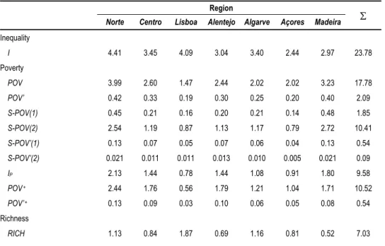
As emphasized above, the measures proposed in Section 2 allow their decomposition by any household’s characteristic, such as type of household (dimension and compo-sition), region of residence, or variables associated with the individual of reference of that household (i.e. the individual with the largest proportion of the annual net total income of the household), such as age, gender, educational level, labor market state, among others. We have conducted a decomposition by region of residence to illu-strate that possibility. This exercise allows focusing on the existence of regional in-equalities in Portugal for the dimensions analysed in this paper.

Table 5 illustrates the decomposition by region of all the measures calculated in Table 3. Additionally, the last row presents evidence in relation to



  N i 1 i i ) (  , allowing us to emphasize the regions where households’ weight in terms of income exceeds their respective weight in terms of dimension.

Table 5 Regional Decomposition of Inequality, Poverty, and Richness Indicators Region



Norte Centro Lisboa Alentejo Algarve Açores Madeira

Inequality I 4.41 3.45 4.09 3.04 3.40 2.44 2.97 23.78 Poverty POV 3.99 2.60 1.47 2.44 2.02 2.02 3.23 17.78 POV’ 0.42 0.33 0.19 0.30 0.25 0.20 0.40 2.09 S-POV(1) 0.45 0.21 0.16 0.20 0.21 0.14 0.48 1.85 S-POV(2) 2.54 1.19 0.87 1.13 1.17 0.79 2.72 10.41 S-POV’(1) 0.13 0.07 0.05 0.07 0.06 0.04 0.13 0.54 S-POV’(2) 0.021 0.011 0.011 0.013 0.010 0.005 0.021 0.09 IP 2.13 1.44 0.78 1.44 1.08 0.91 1.80 9.58 POV+ _{2.44 1.76 0.56 1.79 1.21 1.04 1.71 10.52} POV’+ _{0.13 0.09 0.03 0.10 0.06 0.05 0.08 0.54} Richness RICH 1.13 0.84 1.87 0.69 1.16 0.81 0.52 7.03

(18)

548 Nuno Crespo, Sandrina B. Moreira and Nadia Simoes RICH’ 0.97 1.00 2.54 0.47 0.99 0.85 0.38 7.18 E-RICH(1) 0.13 0.09 0.31 0.04 0.09 0.09 0.03 0.77 E-RICH(2) 1.81 1.30 4.36 0.50 1.30 1.30 0.40 10.98 E-RICH’(1) 0.41 0.48 1.32 0.11 0.30 0.46 0.08 3.17 E-RICH’(2) 0.16 0.27 0.69 0.04 0.11 0.28 0.03 1.59 IR 2.10 1.81 4.33 1.05 1.96 1.90 0.73 13.88

IMC 2.85 2.21 1.96 2.21 2.29 1.40 2.05 14.97    N i 1 i i ) (  -1.74 -0.72 4.37 -1.22 0.96 0.34 -1.99 0

Source: Own calculations based on IDEF. The reading of both incidence and intensity indicators is immediate. The value corresponding to each region should be interpreted in the same way as the overall indicator, though applied exclusively to the given region. Let us consider the poverty indicators as examples. Regarding POV, we found a poverty incidence at the national level of 17.78%. A disaggregation by regions reveals that 3.99% of the individuals from the sample are poor living in the Norte region, 2.60% in the Centro, 1.47% in the region of Lisboa, etc. Adding up the values of the different regions we obtain the incidence of poverty at the national level. We should note, however, that this concept differs from the measurement of poverty incidence within the context of each given region.

In the same vein, regarding POV’, we can say for instance that the amount ne-cessary to eradicate poverty in the Algarve corresponds to (at least) 0.25% of the to-tal income in the economy, while for Madeira that value is equivalent to 0.40% of the total income in the economy. In the national total, as has been seen, a mobiliza-tion of 2.09% of the total income in the economy is needed to overcome poverty. The interpretation made for the values of POV and POVʹ is also valid for the other inci-dence or intensity indicators: S-POV(1), S-POV(2), S-POVʹ(1), S-POVʹ(2), POV+_,

POVʹ+, RICH, RICHʹ, E-RICH(1), E-RICH(2), E-RICHʹ(1), and E-RICHʹ(2). Concerning the inequality indicators (I, IP, IR, and IMC), the value for each

re-gion expresses half of the deviation assigned to households of that rere-gion in relation to an egalitarian situation (having the same weight in terms of income and equivalent adults). So, for instance, taking into account the overall indicator of inequality (I), the deviation from the egalitarian situation of households living in the Norte region equals 8.82% of the total income in the economy.

The percentage of the total income in the economy needed to eradicate inequa-lity within each region cannot, in this case, be identified, because there are inter-regional transfers of income apart from intra-inter-regional transfers. The transfers be-tween regions are net positive amounts transferred to other regions when

0 ) ( 1  



 N i i i 

 and net positive amounts received from other regions in the opposite case.

(19)

Finally, looking at the last row of Table 5, we can identify three regions (Lis-boa, Algarve, and Açores) in which the weight in overall income is greater than the corresponding weight in equivalent adults. Lisboa - the most developed region in the country - has the greatest difference. On the contrary, Madeira shows the most sig-nificant negative deviation.

4. Final Remarks

The main contribution of this paper is the proposal of an integrated approach for the measurement of inequality, poverty, and richness that allows us to derive measures for all these phenomena from a common conceptual framework. We have proposed a set of indicators characterized by their simplicity in application, neutrality, and de-composability. Another important characteristic of the measures proposed in this study is that they allow a concrete economic interpretation of the results, thereby contributing to a more adequate definition of social policies.

The proposed measures were applied, for illustrative purposes, to the Portu-guese economy. Taking total income as a reference, that application has identified 17.78% of individuals in poor households, 7.03% in rich households, and the remain-ing 75.19% in the middle class. A severe poverty situation was found in 1.85% of the individuals analyzed (10.41% of the poor). Particularly important in quantitative terms is the near-poverty phenomenon, accounting for 10.52% of the population which is in accordance with the well-known asymmetric distribution of income. Concerning inequality, we have calculated the need to redistribute (at least) 23.78% of the total income in the economy to reach a full equality situation. With a focus on poverty intensity and providing a very strong policy message, we conclude that 2.09% of the total income in the economy is the amount needed to be transferred from the non-poor to the poor in order to eradicate poverty. Additionally, the com-parison between the results obtained with monetary income and total income stresses significant differences, highlighting the importance of taking into account this last concept of income.

The proposed measures can be decomposed with reference to a given charac-teristic of the household. We have illustrated that property by considering a regional decomposition that includes the seven Portuguese NUTS II regions. In that analysis we found the region of Lisboa (the most developed region in the country) to be the most favorable in terms of poverty and richness.

Regarding the topics developed in this paper, important research avenues re-main. In methodological terms, the main challenge resides in testing the robustness of the results based on alternative values for the parameters in order to check the sen-sitivity of these results. This is especially important for the parameters that distin-guish the main income categories (, , , , and ), that is, poor, rich, middle class, severely poor, extremely rich, and near-poor.

In applied terms, there are several promising areas of research, calling for new contributions. First, cross-country comparative studies would raise the knowledge on the phenomena under examination for a wide range of countries with differing characteristics. Second, the same comparative analysis could be conducted at the regional level, emphasizing and characterizing the specific traits of regional

(20)

inequalities prevailing within a given country. Our results suggest that regional asymmetries have a considerable and significant expression and if this is the case for a small country such as Portugal, it deserves attention in similar and larger territories. Third, an issue that has some contact points with the former is the decomposition of the proposed set of indicators using other household characteristics. Some of the most interesting would be the main source of income of the household (capital, labor, or social benefits) or the level of education of the individual of reference of the household. This is closely related to the understanding of the determinants of poverty and richness, which is crucial knowledge for policy makers to be able to assess the most effective allocation of resources in this area and make a comparative assessment of the impact of alternative policy measures. A fourth important research line that can also be explored taking this paper as departure point is the analysis of a multidimensional concept of poverty and richness. The analysis of these phenomena gains from using a broader lens, going beyond the monetary dimension and also at-tending to other dimensions such as education and health, among others. This could be complemented with national surveys to assess how persons from a given country / society value and therefore rank this set of issues, giving the researcher the informa-tion that is needed to weight and summarize the different aspects considered.

(21)

References

Alvaredo, Facundo, Anthony B. Atkinson, Thomas Piketty, and Emmanuel Saez. 2013.

“The Top 1% in International and Historical Perspective.” Journal of Economic

Perspectives, 27(3): 1-21.

Amiel, Yoram, and Frank A. Cowell. 1992. “Measurement of Income Inequality:

Experimental Test by Questionnaire.” Journal of Public Economics, 47(1): 3-26.

Atkinson, Anthony B. 2007. “Measuring Top Incomes: Methodological Issues.” In Top

Incomes over the Twentieth Century: A Contrast between European and English-Speaking Countries, ed. Anthony B. Atkinson and Thomas Piketty, 18-42. Oxford:

Oxford University Press.

Atkinson, Anthony B., and Thomas Piketty. 2010. Top Incomes: A Global Perspective.

Oxford: Oxford University Press.

Atkinson, Anthony B., and Andrea Brandolini. 2011. “On the Identification of the ‘Middle

Class’.” Society for the Study of Economic Inequality Working Paper 2011-217.

Atkinson, Anthony B., and Andrew Leigh. 2013. “The Distribution of Top Incomes in Five

Anglo‐Saxon Countries over the Long Run.” Economic Record, 89(S1): 31-47.

Atkinson, Anthony B. 2015. Inequality: What Can Be Done? Cambridge, MA: Harvard

University Press.

Bellù, Lorenzo G., and Paolo Liberati. 2006. “Inequality and Axioms for Its Measurement.”

http://www.fao.org/docs/up/easypol/447/inqulty_axms_msrmnt_054en.pdf.

Birdsall, Nancy, Nora C. Lustig, and Christian J. Meyer. 2014. “The Strugglers: The New

Poor in Latin America?” World Development, 60(C): 132-146.

Celidoni, Martina. 2013. “Vulnerability to Poverty: An Empirical Comparison of Alternative

Measures.” Applied Economics, 45(12): 1493-1506.

Chateauneuf, Alain, and Patrick Moyes. 2006. “Measuring Inequality without the

Pigou-Dalton Condition.” In Inequality, Poverty and Well-Being, ed. Mark McGillivray, 22-65. New York: Palgrave Macmillan.

Cowell, Frank A., and Kiyoshi Kuga. 1981a. “Additivity and the Entropy Concept: An

Axiomatic Approach to Inequality Measurement.” Journal of Economic Theory, 25(1): 131-143.

Cowell, Frank A., and Kiyoshi Kuga. 1981b. “Inequality Measurement: An Axiomatic

Approach.” European Economic Review, 15(3): 287-305.

Cowell, Frank A. 2011. Measuring Inequality. 3rd ed. Oxford: Oxford University Press. Dutta, Indranil, James Foster, and Ajit Mishra. 2011. “On Measuring Vulnerability to

Poverty.” Social Choice and Welfare, 37(4): 743-761.

Fields, Gary, and John C. H. Fei. 1978. “On Inequality Comparisons.” Econometrica, 46(2):

303-316.

Foster, James, Joel Greer, and Erik Thorbecke. 1984. “A Class of Decomposable Poverty

Measures.” Econometrica, 52(3): 761-776.

Gaertner, Wulf, and Ceema Namezie. 2003. “Income Inequality, Risk, and the Transfer

Principle: A Questionnaire-Experimental Investigation.” Mathematical Social Science, 45(2): 229-245.

Guimarães, Ricardo. 2007. “Searching for the Vulnerable: A Review of the Concepts and

Assessments of Vulnerability Related to Poverty.” European Journal of Development

(22)

Haughton, Jonathan, and Shahidur R. Khandker. 2009. Handbook on Poverty and

Inequality. Washington, DC: World Bank.

Magdalou, Brice, and Patrick Moyes. 2009. “Deprivation, Welfare and Inequality.” Social

Choice and Welfare, 32(2): 253-273.

Magdalou, Brice, and Richard Nock. 2011. “Income Distributions and Decomposable

Divergence Measures.” Journal of Economic Theory, 146(6): 2440-2454.

Medeiros, Marcelo. 2006. “The Rich and the Poor: The Construction of an Affluence Line

from the Poverty Line.” Social Indicators Research, 78(1): 1-18.

Paulus, Alari, Holly Sutherland, and Panos Tsakloglou. 2010. “The Distributional Impact

of In-Kind Public Benefits in European Countries.” Journal of Policy Analysis and

Management, 29(2): 243-266.

Peichl, Andreas, Thilo Schaefer, and Christoph Scheicher. 2010. “Measuring Richness and

Poverty: A Micro Data Application to Europe and Germany.” Review of Income and

Wealth, 56(3): 597-619.

Piketty, Thomas. 2005. “Top Income Shares in the Long Run: An Overview.” Journal of the

European Economic Association, 3(2-3): 382-392.

Piketty, Thomas, and Emmanuel Saez. 2006. “The Evolution of Top Incomes: A Historical

and International Perspective.” American Economic Review, 96(2): 200-205.

Piketty, Thomas. 2014. Capital in the Twenty-First Century. Cambridge, MA: Harvard

University Press.

Piketty, Thomas, and Emmanuel Saez. 2014. “Inequality in the Long Run.” Science,

344(6186): 838-843.

Pritchett, Lant, Asep Suryahadi, and Sudarno Sumarto. 2000. “Quantifying Vulnerability

to Poverty: A Proposed Measure, Applied to Indonesia.” World Bank Policy Research Working Paper 2437.

Ravallion, Martin. 2003. “The Debate on Globalization, Poverty and Inequality: Why

Measurement Matters.” International Affairs, 79(4): 739-753.

Roine, Jesper, and Daniel Waldenström. 2008. “The Evolution of Top Incomes in an

Egalitarian Society: Sweden, 1903-2004.” Journal of Public Economics, 92(1-2): 366-387.

Saez, Emmanuel, and Gabriel Zucman. 2014. “Wealth Inequality in the United States since

1913: Evidence from Capitalized Income Tax Data.” National Bureau of Economic Research Working Paper 20625.

Salverda, Wiemer, Brian Nolan, and Timothy M. Smeeding. 2011. The Oxford Handbook

of Economic Inequality. Oxford: Oxford University Press.

Sen, Amartya. 1976. “Poverty: An Ordinal Approach to Measurement.” Econometrica,

(23)

Appendix

Richness and Middle Class Inequality

Let us define RICH as the ratio between the number of individuals in rich households and the total number of individuals:

. 1 ) ( 1



    _N i i N R Si i H H RICH i (21)

To obtain a measure of richness intensity, we define: .

i i

i  

   (22)

Then, richness intensity is given by:

,

'

) ( 1



 



N R Si i i

RICH



₍₂₃₎

representing the percentage of the total income in the economy according to which the rich are above the richness line. Dividing RICHʹ by the number of rich house-holds we can obtain the average intensity of richness.

Finally, we attend to richness depth. We do so using the same approach we have applied in the poverty case. As a first step, we define an extreme richness line, above which households are classified as extremely rich:

,

if







_



i i i

ER

S

(24)

in which > 1. The logic behind the definition of this threshold is very similar to that presented in the main text for the case of poverty.

The incidence of extreme richness can be expressed in relation to either the to-tal population or the rich population. In each case we have, respectively:

, ) 1 ( 1 ) ( 1



    _N i i N ER Si i H H RICH E i (25) and

(24)

554 Nuno Crespo, Sandrina B. Moreira and Nadia Simoes . ) 2 ( ) ( 1 ) ( 1



     _N R Si i N ER Si i i i H H RICH E (26)

In turn, taking as reference either the richness line or the extreme richness line, the intensity of extreme richness can be defined respectively as:

, ) 1 ( ' ) ( 1



    N ER Si i i RICH E  ₍₂₇₎ and , ) 2 ( ' ) ( 1



    N ER Si i i RICH E  ₍₂₈₎

where



_i is expressed in (22) and:

.

i i

i  

   (29)

As in the case of the severity of poverty, we can also calculate an inequality measure applied exclusively to the rich population, aiming to determine the amount of income that it is necessary to redistribute among the rich in order to equalize the distance of each rich individual to the richness line:

,

) ( 1



 





N R Si i i R i

I







₍₃₀₎ in which: , ) ( 1



   _N R Si i i i i Y Y



(31) and . ) ( 1



  _N R Si i i i i D D  (32)

Regarding the evaluation of the middle class inequality, we start by focusing on households in which Si_{= MC, calculating:}

(25)

,

) ( 1









N MC Si i i MC i

I







₍₃₃₎ in which: , ) ( 1



   _N MC Si i i i i Y Y



(34) and . ) ( 1



  _N MC Si i i i i D D



(35)

τ takes value 0.5, as in the cases of  and k.

IMC is an income inequality measure for the middle class, indicating the

per-centage of the total income of the middle class that, if adequately redistributed among middle class households, would eliminate the inequality in this income group.

(26)