Calibration of the VISSIM truck performance model using GPS data

Calibra on of the VISSIM truck performance model

using GPS data

Luan Guilherme Staichak Carvalho1, José Reynaldo Se#2

1_{Departamento de Engenharia de Transportes, EESC-USP, lgscarvalho@usp.br} 2_{Departamento de Engenharia de Transportes, EESC-USP, jrase0@usp.br}

Recebido:

6 de maio de 2019

Aceito para publicação:

4 de setembro de 2019 Publicado: 12 de novembro de 2019 Editor de área: Flávio Cunto ABSTRACT

Traffic simulators can be used to perform safe, low cost scenario evalua on. However, their mathema cal models are calibrated to scenarios commonly found in the simula-tors’ country of origin. VISSIM truck accelera on func ons were created for trucks with be:er power/mass ra os than typical Brazilian trucks. This paper presents the

calibra-on of VISSIM truck accelera calibra-on func calibra-ons using the difference between real and simu-lated speed profiles as goodness-of-fit measures. Using GPS, speed profiles were ob-tained for 57 trucks travelling over a segment of 18 km, four-lane freeway situated on rolling terrain, under low traffic flow. The calibra on procedure was automated and based on a gene c algorithm. Several calibra on runs were performed using different numbers of genera ons and popula on size. The resul ng accelera on func ons are presented and discussed.

RESUMO

Simuladores de tráfego permitem avaliar cenários de maneira segura e com baixo custo. Todavia, os modelos matemá cos que os regem são ajustados para cenários frequentes no país de origem do simulador. No VISSIM, os modelos referentes ao deslocamento de caminhões simulam veículos com melhor desempenho, se comparados aos caminhões brasileiros. Este trabalho apresenta a calibração das funções de aceleração para cami-nhões do VISSIM, u lizando a diferença entre perfis de velocidade simulados e reais como medidas de ajuste. Usando GPS, foram ob dos perfis individuais para 57 cami-nhões que trafegaram por cerca de 18 km ao longo de uma rodovia de pista dupla em relevo ondulado, sob baixo fluxo de tráfego. A calibração foi automa zada por meio de um algoritmo gené co. Diversas execuções do algoritmo foram realizadas, variando nú-mero de gerações e tamanho populacional. As funções de aceleração ob das são apre-sentadas e discu das.

Keywords:

Traffic stream simula on, VISSIM, GPS, Vehicular performance, Calibra on of microsimula on models, Trucks. Palavras-chaves:

Simulação de Correntes de Tráfego, VISSIM, GPS, Desempenho veicular, Calibração de microssimuladores de tráfego, Caminhões. DOI:10.14295/transportes.v27i3.2042

1. INTRODUCTION

Computional simulation models are used in different areas of science because they can predict, reproduce and assess real and hypothetical scenarios. In traf ic studies, widespread use of these tools can be explained by the low cost, the fact that they are risk-free and the speed in which data are obtained (Park and Qi, 2005). By combining different mathematical models, simulators are able to reproduce real phenomena of great complexity. This ability leads to the study and evaluation of the theories behind these phenomena by comparing them with simulated scenar-ios (Heermann, 1990).

Simulators present one or more default setting sets for each of their mathematical models. Each set is made in such a way that the reproduction of speci ic traf ic scenarios – usually con-sistent with the leet and the drivers of the simulator’s country of origin – reproduces the real traf ic low with a satisfactory degree of idelity. However, the vehicles’ characteristics and be-havior can vary not only from one country to another, but also between regions within the same country. Therefore, simulators should be calibrated according to the conditions of the place of study in order to ensure the reliability of the simulated data (Hourdakis et al., 2003).

In Brazil, most efforts made to calibrate simulators focus on models that govern interactions among vehicles (Egami et al., 2004; Medeiros et al., 2013; Bethonico et al., 2016), and there are few studies actually addressing vehicle performance calibration (Cunha et al., 2009). Therefore, the aim of this paper is to calibrate the VISSIM vehicle performance model for Brazilian trucks. To do this, a real freeway segment of rolling terrain, approximately 18 km long, was used. The calibration was carried out by comparing the speed pro iles of real and simulated trucks trav-elling along the segment under study, where the real instantaneous speeds were obtained from GPS data processing. The calibration was automated using a genetic algorithm as this technique is widely cited in the literature concerning traf ic simulator calibration (Kim & Rilett, 2001; Ma & Abulhai, 2002; Egami et al., 2004; Cunha et al., 2009; Medeiros et al., 2013; Chiappone et al., 2016).

2. TRAFFIC SIMULATORS AND THE NEED TO CALIBRATE THEM

Computational simulators are often cited in the literature and have appeared as both objects and tools for studies in different areas of science for over 50 years (Shumate and Dirksen, 1965). Despite the long history of studies on traf ic simulators, the need to calibrate them has become a recurrent topic only since the late 1990s. The 30-year time lag of this topic in relation to the beginning of when these tools were used in the transport sector can be explained by the way these programs were developed. The irst traf ic simulators were created and validated to sim-ulate one or a few speci ic scenarios, whereas their successors were designed to reproduce in-creasingly broader conditions (Kotusevski and Hawick, 2009). As current simulators are cre-ated and validcre-ated to simulate generic networks, calibration has become necessary to better represent behaviors observed in local scenarios (Jayakrishnan et al., 2001; Hourdakis et al., 2003).

Among the various attempts to calibrate simulator models, the most frequent ones are the car-following and lane-change models (Chu et al., 2003). However, the large number of variables and the high computational costs required for calibration mean that, generally, models are not calibrated regularly. Therefore, the frequent use of simulators occurs only by adjusting the origin-destination matrices and changing a few behavioral variables based on the user’s expe-rience (Balakrishna et al., 2007).

In traf ic microsimulators, the models involved recreate the traf ic low by generating vehi-cles with individual behaviors. Thus, using aggregate traf ic measurements to calibrate these models is not appropriate since aggregate measurements are affected by the combination of several models simultaneously (Toledo et al., 2004). On the other hand, disaggregate data is dif icult to collect and costly (Balakrishna et al., 2007), making it complex to calibrate simula-tors. Despite this dif iculty, Li et al. (2015) carried out the calibration of the VISSIM desired ac-celeration function for passenger cars using GPS data obtained for individual vehicles travelling on urban roads. Hence, it is expected that this approach can be applied for freeway segments.

In order to calibrate vehicle performance models, common procedures include simulating segments comprising a long ramp preceeded by a lat section in which the truck’s speed stabi-lizes (Cunha et al., 2009). Although this approach makes it possible to compare the equilibrium speed, such a combination of ramps rarely occurs since the rolling terrain, characterized by the constant alternation between up grades and down grades, is the most common scenario.

In this research, these shortcomings were avoided by collecting data in a more realistic way, using a GPS device installed on a sample of trucks that travelled along a divided multilane high-way during periods of low traf ic low. With the set of instantaneous speed pro iles thus ob-tained, the truck performance model used by VISSIM was recalibrated using a genetic algorithm.

3. VISSIM TRUCK PERFORMANCE MODEL

In VISSIM, vehicles can change speed through acceleration functions, which in turn are created for each vehicle based on their category from pre-con igured functions, as shown in Figure 1. These functions represent a region of possible acceleration values in relation to the vehicle’s instantaneous speed. For heavy vehicles, these regions are delimited by acceleration functions that correspond to the limits for the power/mass ratio. For the VISSIM default setting, the upper and lower limits are 7 and 30 kW/t, respectively (PTV, 2016).

Figure 1. Default maximum acceleration and desired acceleration functions for heavy vehicles in VISSIM 9 [Adapted

from PTV (2016)].

In order to de ine the acceleration versus the available speed values for a simulated truck, VISSIM calculates the power/mass ratio of that vehicle the moment it is generated. The obtained value is then compared with the upper and lower limits of the power/mass ratio set for the simulation. If the truck’s power/mass ratio is not within the limits, the calculated value is re-placed by the nearest limit; for example, in the setting shown in Figure 1, the power/mass ratio of a truck with 4 kW/t will be rounded up to 7 kW/t as that is the limit closest to the calculated value. In this case, the vehicle’s maximum acceleration and desired acceleration values will be equal to the respective limit-curves for its new power/mass value.

If the truck’s power/mass is within the limits, its acceleration values will be obtained by lin-ear interpolation between the limit-curves, using the truck’s power/mass as a measure of dis-tance for interpolation. In Figure 1, the "median" curves correspond to the interpolated accel-erations for a truck with 18.5 kW/t, whereas the limit-curves are the accelaccel-erations used by trucks outside the stipulated power/mass range.

Apart from the differences in mass and power among trucks, VISSIM also varies the possible acceleration based on the slope of the ramps. Whenever a vehicle is travelling on steep grades, its maximum acceleration curve is displaced vertically, changing each point through the relation

av,G = (av – 0.1G), where av is the acceleration (in m/s²) at speed v on a lat stretch; and av,G is the

acceleration (in m/s²) at speed v in an ascending grade of magnitude G (in m/100 m).

Another important aspect of this simulator is that all the vehicles receive a desired speed value when they are created. The desired speed determines the highest speed the vehicle will reach, even when the interpolated acceleration curves allow it to reach higher speeds.

4. THE APPROACH USED

The VISSIM default setting provides only one category for trucks. However, the Brazilian leet is heterogeneous, and each vehicle can present quite varied combinations of characteristics (power, mass, number of axles, age, maintenance conditions, and so on). Therefore, calibrating acceleration functions for more than one category of trucks is a way of obtaining more appro-priate results for subgroups that share common characteristics. This work follows the classi i-cation of Brazilian trucks as proposed by Cunha et al. (2008), dividing them into four types: light (2 axles); medium (3 axles); heavy (4 and 5 axles) and extra-heavy trucks (6 or more axles).

As the acceleration functions govern the independent displacement of the vehicles, i.e. as if they did not suffer interaction from traf ic, in order to calibrate the simulator, real data from trucks travelling under these conditions need to be obtained. Carvalho and Setti (2017) present a method for collecting, treating and obtaining speed pro iles of individual vehicles, which can be used as a measure for adjusting the functions.

However, VISSIM is a stochastic simulator, in which the mass, power and desired speed (MPdS) values of each vehicle are random variables, generated from cumulative frequency dis-tributions for that truck’s class. Consequently, cross-checking the real and simulated speed pro-iles under these conditions would not produce a satisfactory calibration, as the MPdS proper-ties of the trucks being compared would be different from each other. Thus, a non-stochastic con iguration of the simulator needs to be obtained for the calibration.

By default, VISSIM vehicle types correspond to vehicle categories (for ex.: Type 1 – passenger cars, Type 2 – trucks). At the beginning of a simulation run, three cumulative frequency distri-butions (one for each MPdS characteristic) and one set of acceleration functions are assigned to each vehicle type.

In order to make it possible to compare real and simulated vehicles with equal MPdS values, the concept of VISSIM vehicle types was modi ied, making each type correspond to an observed truck, i.e. with known and constant MPdS values. Trucks from the same category use the same set of acceleration functions, allowing these functions to be calibrated simulating all trucks that belong to this category.

Therefore, the MPdS distributions still need to be con igured for each truck so that they use ixed values, preventing the generation of random vehicles. The distributions were con igured as two pairs of values: Y (0%), for the cumulative frequency 0%; and Y (100%), for the cumula-tive frequency of 100%. As VISSIM does not allow Y (0%) = Y (100%), it was assumed that Y (0%) = Y (100%) − 0.001, so that the MPdS property value is constant, regardless of the value selected by the distribution.

5. PROPOSED METHOD

Brie ly, the calibration was obtained using a genetic algorithm whereby each individual is a pos-sible combination of values for the limit-curves that comprise the maximum and desired accel-eration functions. The presentation of the method begins by addressing two important aspects of the genetic algorithm: the real data and the itness function, calculated at the end of the eval-uation function. Afterwards, the procedure to create the four networks (one for each truck cat-egory) in the simulator is described. Then, the implementation of the genetic algorithm is dis-cussed. Finally, the validation of the acceleration functions is addressed.

5.1. Input data

Speed pro iles are used to assess the acceleration function itness. The sample consisted of 57 trucks travelling on a divided, multilane highway, with a posted speed limit of 90 km/h for trucks. The road segment chosen for the data collection is located in rolling terrain and its ver-tical alignment consists of a sucession of crest and sag verver-tical curves connected by grades of varied lengths and magnitudes. The horizontal alignment of this road segment is straight, with-out any horizontal curves.

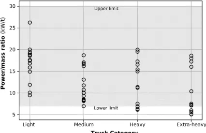
Truck drivers were approached at a mobile weigh station and, upon their agreement in par-ticipating in the data collection, a researcher would board the truck and install the GPS unit and antenna. The drivers were asked to drive as they usually would do in that segment. The GPS unit recorded the vehicle location at 1-second intervals. The data collection was conducted during periods when the traf ic low was low, to prevent speed reductions due to the traf ic. Truck mass was obtained from the weigh station scale; the engine power and number of axles were ob-tained from a short interview with the driver. Figure 2 shows the power/mass ratio for the trucks in the sample, according to their category. The grey area in the graph shows the upper and lower limits of VISSIM’s default power/mass ratio.

Figure 2. Power/mass ratio for trucks in the sample. The grey area shows VISSIM’s default range for power/mass ratios

(7–30 kW/t).

The method used for constructing the speed pro iles was adapted from Carvalho and Setti (2017), using code written in Python 3.6. Two different speed pro iles were derived for each truck. The irst one characterizes the initial phase of the movement, when the truck is starting

from a complete stop and accelerates to reach the desired speed. It was assumed that this initial phase comprised the irst 1.5 km travelled. It describes the instantaneous speed of the vehicle at predetermined points.

The second pro ile represents the movement of the truck after it reached its desired speed and accelerates or decelerates because of the effect of grades on its path. This speed pro ile was built using the GPS data collected over the 16.5 km segment after the initial 1.5 km section and consists of the instantaneous speeds at 100-m stations along the segment.

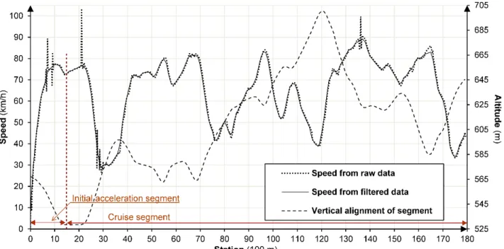
Figure 3 shows the speed pro ile for one of the trucks in the sample. The speeds from iltered data at each station were adopted as the real speeds in the calibration of the truck performance model.

Figure 3. Speed profile representing the observed speeds during the initial acceleration and cruise phases for one of the

trucks used for the data collection (Truck 53).

The desired speed for each truck was de ined as the 90th _{percentile of the cruise speed of the}

respective vehicle. This threshold was adopted after identifying that, despite the observed trucks being able to reach high speeds, they were unable to maintain these high speeds for long distances. Speeds near the 90th _{percentile, however, were more easily sustained by most trucks}

and thus considered more representative of the truck’s desired speed.

5.2. Crea;ng simula;on networks

The simulation network was created using the path of a randomly chosen truck as the reference for the horizontal and vertical alignments of the highway. This highway segment was repro-duced in the simulation by one 18-km link with one single traf ic lane. To optimize the simula-tion runs, the network used comprised two identical 18-km links, one that was used to analyze the initial acceleration phase of the trip and the other for the cruise phase of the trip. To collect the data to characterize the performance of the simulated trucks, dual-loops detectors measured the speed of the truck at predetermined points along the network links. In the link

representing the initial acceleration phase, the detectors were placed at variable distances; in the link used to simulate the cruise phase of the trip, the detectors were placed at 100-m sta-tions. Figure 4 illustrates the network used for the simulation.

Figure 4. Schematic diagram of start and cruise default links.

The simulations used a low of 60 veh/h during the irst minute of the simulation, followed by no additional input lows, ensuring that only one truck per link were simulated, with a total absence of traf ic interaction.

In VISSIM, vehicles whose power/mass ratio is not within the prede ined limits (7 to 30 kW/t) receive an acceleration curve that is equal to the nearest limit. As can be observed in Figure 2, a signi icant part of the power/mass values of the sample are not within VISSIM stand-ard limits. In order to prevent the simulator from disregstand-arding the difference of the vehicles’ performance not included in this range, the decision was to change the power/mass ratio limits to 2.3 and 23.2 kW/t.

Finally, the simulation time was set to 40 minutes, which is approximately double what is required for the real trucks to complete the route along the segment.

5.3. Fitness func;on

The itness function, i.e. the function that returns the quality measure of the calibrated acceler-ation functions was a combinacceler-ation of two error measures, calculated for the two speed pro iles (the initial acceleration phase and the cruise phase).

The irst error measure uses the average error between real (observed) and simulated speeds in order to obtain an average error close to zero. This measure is represented by:

= 1 1 − ,

where µ: the mean average of the simple errors for the speed of each truck;

c: the index that represents the trucks belonging to the category (light,

medium, heavy or extra-heavy);

N: the total number of trucks for that category;

i: the index that represents the station along the way;

M(c): the number of stations through which the c-th vehicle travelled;

: the simulated speed of the c-th truck at the i-th station along the segment; and : the observed speed of the c-th truck at the i-th station along the segment.

The second measure uses square errors to penalize the larger differences between real and simulated speeds at each station:

= 1 1 − ,

where ε is the square root of the mean average of the squared errors in the speed observation of each truck and all the other parameters were de ined in Eq. 1.

Finally, the itness function, which measures the quality of the calibration, is calculated through the function:

= + + ! +₄

where F is the itness for an individual (i.e. a given set of calibration parameters from the per-formance model) in the population which comprises the current generation; a and c indicate the acceleration and cruise segments, respectively, for which the measurements µ and ε are cal-culated; and p is the penalty factor for measurement ε in the accelerating segment (where the initial acceleration occurs). The p value was empirically ixed at 0.2 because it was detected that this measurement could represent about 80% of the itness, which would virtually eliminate the contribution of the other measures in the total value of F, hindering the calibration of the acceleration functions.

5.4. Implemen;ng the Gene;c Algorithm

A genetic algorithm is a search heuristic based on the process of natural selection. The genetic algorithm used to search for the best values for the acceleration functions was coded in Python v. 3.6 using the Spyder v. 3.2.6 development environment. Figure 5 shows a lowchart of the general structure of the genetic algorithm (GA) used.

Figure 5. General flowchart of the genetic algorithm used to recalibrate the truck performance model.

(2)

The program contains three modules. The control module contains the routines to control the search and call the other two modules when needed. The second module is used to apply the genetic operators (selection, crossover, mutation and predation) used to create new indi-viduals from the current population. The third module is used to calculate the itness function value of an individual, a process that requires running VISSIM with new values for the maximum and desired acceleration functions to produce a simulated speed pro ile.

Selection of individuals for crossover assumes that all individuals in the previous generation are able to reproduce; best itted individuals, however, have a greater chance to be selected, as the selection is based on the individual’s itness value. Routines for crossover, mutation and creating new individuals include a series of constraints, because VISSIM requires the accelera-tion funcaccelera-tions to have the characteristic format shown in Figure 1. Those constraints also pre-vent the GA from creating acceleration values that would represent unrealistic operating con-ditions for the trucks. The best individual in each generation is always preserved, so the itness value of the best individual in every generation is either maintained or improved and never worsens.

The creation and modi ication of individuals considered only the upper and lower limits of the acceleration functions. This decision reduced the constraints on the application of genetic operators when creating a new generation and increased the genetic variability of the popula-tions. When needed, the median function is obtained from the average between the lower and upper acceleration limits for a given speed.

In each generation, 30% of the population (excepting the best individual) were randomly selected for mutation. Once an individual is selected for mutation, each of its genes had a 20% chance of being mutated. Mutation was carried out by attempting to add a random number be-tween ±0.2 m/s² to the gene selected for mutation. If the new value was not valid, a new random value was selected, and the new sum was veri ied. The procedure is repeated up to ive times and if none of the attempts resulted in a valid new gene, the original gene value was kept.

Predation was applied at every generation corresponding to 1/10 of the number of genera-tions chosen for the GA run. At each predation, individuals were ranked according to their it-ness function value and the individuals in the lower quartile were replace by new, randomly generated individuals.

The itness function evaluation consists of the following stages: inserting the acceleration functions’ parameters into VISSIM, simulating the network with the con iguration of the indi-vidual’s acceleration functions; reading the simulation outputs; extracting detector speeds from the report; and calculating the individual’s itness.

The criterion for stopping the search was the number of generations, as the overall objective was to obtain the best itness possible. At the end of its execution, the genetic algorithm issues two reports. The irst one contains the con igurations of the algorithm, the maximum and de-sired acceleration functions for the best individual, the measurement of its itness and the met-rics concerning the crossover and mutation operations. The second report contains the best and worst individuals of each generation, as well as the maximum, average, minimum and standard deviation of the itness of each population.

To validate the calibration, 12 out of the 57 trucks were removed from the calibration phase, 3 from each category. The performance models for each truck category were calibrated sepa-rately from each other. Several combinations of population size and number of generations were analyzed to ind the one that delivered a good level of itness with an acceptable processing

time. The combinations chosen for this study were: (1) population size of 85 individuals and 85 generations, which required 7423 evaluations of the itness function; and (2) population of 105 individuals and 105 generations, demanding 11268 calculations of the itness function value.

6. RESULTS ANALYSIS

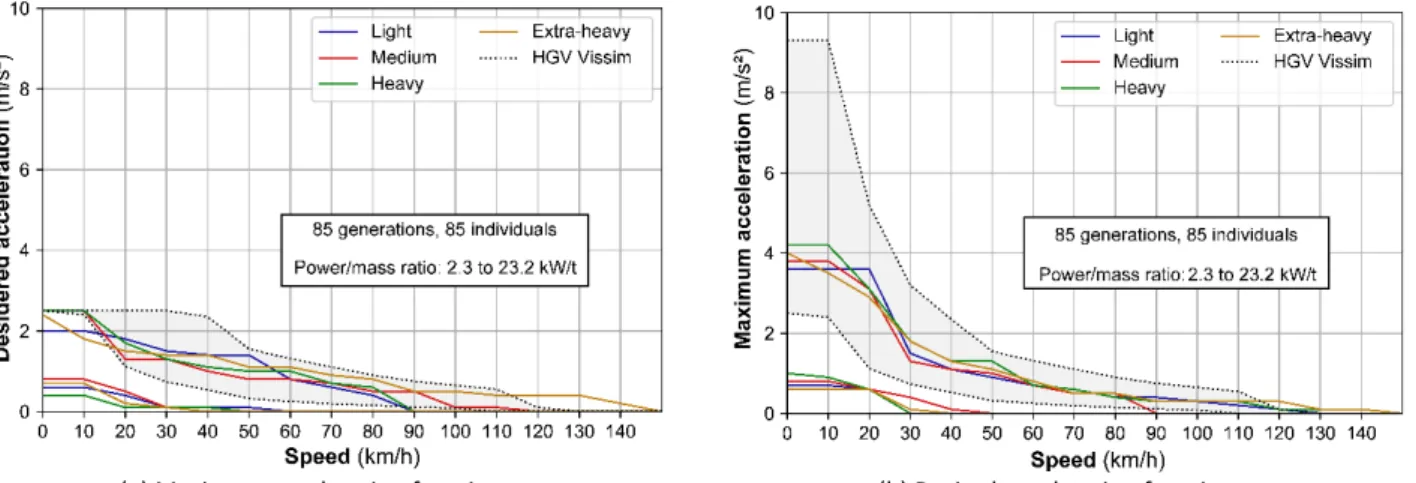
Figures 6 and 7 show the default values for the maximum and desired acceleration functions (shown as HGV Vissim), as well as the best con igurations for the four categories of trucks ob-tained for two combinations of numbers of generations and population size. The limits of the calibrated acceleration functions refer to power/mass ratios ranging between 2.3 and 23.2 kW/t, whereas the VISSIM default functions assume power/mass ratios from 7 to 30 kW/t.

(a) Maximum accelera on func ons (b) Desired accelera on func ons Figure 6. Maximum and desired acceleration functions obtained from 85 generations and 85 individuals.

(a) Maximum accelera on func ons (b) Desired accelera on func ons

Figure 7. Maximum and desired acceleration functions obtained from 105 generations and 105 individuals.

It can be observed that, in general, the calibrated maximum acceleration functions are similar in format to the originals for speeds between 30 and 80 km/h. However, the calibrated values are slightly lower. Two hypotheses are raised to explain this phenomenon. First, it is likely that lower values are caused because the sampled trucks did not use all the engine power. As the drivers were not asked to drive in a speci ic way, they probably did not use all the power pro-vided by the engines. Therefore, the obtained acceleration values refer to the use of the power desired by the drivers rather than the maximum possible power. Furthermore, the maximum

power depends on the engine’s conditions (maintenance, age, etc.) and, therefore, the resulting functions are affected by the difference between nominal and real power. This hypothesis is corroborated by the maximum acceleration functions presented in Figure 6 and Figure 7, which are always lower than the original ones.

The calibrated desired acceleration function presented upper limits with a similar format to the original, between 0 and 80 km/h. At the lower limits, the accelerations between 0 and 60 km/h are signi icantly lower than the default con iguration, which suggests that the drivers were not using the maximum power.

It was observed that, in general, the different combinations of the number of generations/ population size generated calibrated functions with formats similar to each other for the range from 0 to 90 km/h. However, the acceleration values for speeds above 90 km/h differed signi i-cantly between the algorithm alternatives (number of generations, population size, among other issues), for the same category of trucks. This can be observed by comparing the functions in Figure 6 with those in Figure 7. This is probably because there are few observations of real speeds above 90 km/h.

Figure 8 shows the real and simulated speed pro iles for the same truck. It can be observed that the simulated speed pro iles are limited by the desired speed. It can also be noticed that the default performance model tends to overestimate the speed in a signi icant part of the trip, whereas the calibrated model tends to the observed speed. It is also important to notice that VISSIM does not replicate illogical driver behavior, such as the speed reduction applied to the truck between stations 40 and 50 and between stations 155 and 160. Figure 9 also shows that the effect of having a greater population and a greater number of generations is not very notice-able on the recalibrated performance model.

Figure 8. Speed profiles for the same truck showing real and simulated data (Truck 44).

7. VALIDATION OF THE RECALIBRATED MODEL

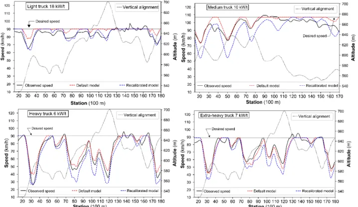
Figure 9 summarizes the validation of the recalibrated truck performance model. The validation consisted in comparing observed and simulated speed pro iles for trucks whose speed data were not used in the model calibration.

The recalibrated models used in the simulations whose results are shown in Figure 9 were derived from the average acceleration values found for the trucks in each category, thus sup-posed to represent a typical truck of that particular type. Consequently, it is normal to ind greater differences in speed during the validation of the model.

Figure 9. Comparison of observed speed profile vs. speed profile obtained with the default model and the recalibrated

model, for four different trucks not included in the sample used for the calibration of the truck performance model.

Figure 9 shows that the behavior of all four trucks is consistent with the observed speed pro ile, except for the illogical speed reductions that VISSIM cannot reproduce well – e.g., be-tween stations 30 and 40 for the medium truck; and bebe-tween stations 40 and 50 for the extra-heavy, the medium and the light trucks.

8. FINAL CONSIDERATIONS

By using the proposed method, the maximum and desired VISSIM acceleration functions for Brazilian trucks could be calibrated. Based on the considerations adopted, it can be observed that the functions have satisfactory values for speeds between 0 and 90 km/h. Moreover, it should be highlighted that the limits for the power/mass ratio should be adjusted when using the calibrated functions.

A suggestion for future calibrations is to conduct an in-depth analysis to adopt the desired speed, given its importance not only for the VISSIM operation, but also for the evaluation of the functions’ adjustment.

Finally, we recommend analyzing the importance of calibrating different functions for each truck category. Increasing the number of executions of the algorithm would enable one to eval-uate how signi icant the differences are between categories. A second implication would be to obtain maximum and desired acceleration functions for a single truck category from the mean values obtained for the segregated truck categories.

ACKNOWLEDGEMENTS

The authors would like to thank Centrovias for the support provided during the data collection. This research received inancial support from CNPq (Grant 312460/17-1) and was funded in part by the Coordenação de Aperfeiçoamento de Pessoal de Nı́vel Superior - Brasil (CAPES) - Funding Code 001.

REFERENCES

Balakrishna, R., C. Antoniou, M. Ben-Akiva, H. Koutsopoulos, and Y. Wen (2007). Calibration of microscopic traf ic simulation models: Methods and application. Transportation Research Record: Journal of the Transportation Research Board, v. 1999, p. 198–207. DOI: 10.3141/1999-21.

Carvalho, L. G. S. and J. R. Setti (2017). Construção de per is de velocidade de caminhões utilizando iltro gaussiano e regres-sões lineares em dados de GPS. In Anais do XXXI Congresso Nacional de Pesquisa em Transporte, ANPET, p. 3341–3352. Chiappone, S.; O. Giuffrè; A. Granà; R. Mauro and A. Sferlazza (2016) Traf ic simulation models calibration using speed–density

relationship: An automated procedure based on genetic algorithm. Expert Systems with Applications, v. 44, p. 147-155, DOI:10.1016/j.eswa.2015.09.024.

Chu, L., H. X. Liu, J.-S. Oh, and W. Recker (2003). A calibration procedure for microscopic traf ic simulation. In: Proc. of the 2003

IEEE International Conference on Intelligent Transportation Systems, Shanghai, China, v. 2, p. 1574–1579. DOI:

10.1109/ITSC.2003.1252749

Cunha, A. L., J. E. Bessa Jr., and J. R. Setti (2009). Genetic algorithm for the calibration of vehicle performance models of micro-scopic traf ic simulators. In: Lopes L., N. Lau, P. Mariano, e L. Rocha (eds) Progress in Arti0icial Intelligence. EPIA 2009. Lec-ture Notes in Computer Science, v. 5816. Springer, Berlin, Heidelberg. DOI: 10.1007/978-3-642-04686-5_1

Cunha, A. L. B. N., M. M. Modotti, and J. R. Setti (2008). Classi icação de caminhões através de agrupamento por análise de clus-ter. In Panorama Nacional da Pesquisa em Transportes 2008, Anais do XXII Congresso de Pesquisa e Ensino em Transportes, ANPET, p. 1447–1459.

Egami, C. Y., J. R. Setti, and L. Rillet (2004). Algoritmo genético para calibração automática de um simulador de tráfego em ro-dovias de pista simples. Transportes, v. 12, n. 2, p. 5–14. DOI: 10.14295/transportes. v12i2.134

Heermann, D. W. (1990). Computer-Simulation Methods. Berlin, Heidelberg: Springer Berlin Heidelberg.

Hourdakis, J., P. Michalopoulos, and J. Kottommannil (2003). Practical procedure for calibrating microscopic traf ic simulation models. Transportation Research Record: Journal of the Transportation Research Board, v. 1852, p. 130–139. DOI:

10.3141/1852-17

Jayakrishnan, R., J. Oh, and A. Sahraoui (2001). Calibration and path dynamics issues in microscopic simulation for advanced traf ic management and information systems. Transportation Research Record: Journal of the Transportation Research

Board, v. 1771, p. 9–17. DOI: 10.3141/1771-02

Kim, K. and L. R. Rilett (2001) Genetic algorithm based approach for calibration of microscopic simulation models. In: Proc. of

the 2001 IEEE Intelligent Transportation Systems Conference, Oakland, CA, USA, p. 698–704.

DOI:10.1109/ITSC.2001.948745

Kotusevski, G. and K. Hawick (2009). A review of traf ic simulation software.

Research Letters in the Information and Mathe-matical Sciences, v. 13, p. 35–54.

Li, J., H. J. Van Zuylen, and X. Xu (2015). Driving type categorizing and microscopic simulation model calibration.

Transporta-tion Research Record: Journal of the Transportation Research Board, v. 2491, p. 53–60. DOI: 10.3141/2491-06

Ma, T. and Abdulhai, B. (2002) Genetic Algorithm-Based Optimization Approach and Generic Tool for Calibrating Traf ic Mi-croscopic Simulation Parameters. Transportation Research Record: Journal of the Transportation Research Board, v. 1800, p. 6–15. DOI: 10.3141/1800-02

Medeiros, A., M. de Castro Neto, C. Loureiro, and J. E. Bessa Jr. (2013). Calibração de redes viárias urbanas microssimuladas com o uso de algoritmos genéticos. In: Anais do XXVII Congresso Nacional de Pesquisa em Transporte, ANPET.

Park, B. and H. Qi (2005). Development and evaluation of a procedure for the calibration of simulation models.

Transporta-tion Research Record: Journal of the Transportation Research Board, v. 1934, p. 208–217. DOI:

10.1177/0361198105193400122

PTV (2016). PTV VISSIM 9 User Manual. Karlsruhe, Germany: PTV Planung Transport Verkehr AG.

Shumate, R. P. and J. R. Dirksen (1965). A simulation system for study of traf ic low behavior. Highway Research Record, v. 72, p. 19–39.

Toledo, T., M. Ben-Akiva, D. Darda, M. Jha, and H. Koutsopoulos (2004). Calibration of microscopic traf ic simulation models with aggregate data. Transportation Research Record: Journal of the Transportation Research Board, v. 1876, p. 10–19. DOI: 10.3141/1876-02