A Work Project, presented as part of the requirements for the Award of a Masters Degree in Finance from the NOVA – School of Business and Economics and
a Professional Master in Finance from the São Paulo School of Economics.
An examination of the cross-sectional relationship of beta and return
in international stock returns: evidence from emerging and developed
markets.
Joshua Patrick Spierts
NOVA-SBE STUDENT NR. 29367 FGV-EESP STUDENT NR. C338715
A Project carried out on the Double Degree EESP-FGV and NOVA-SBE, under the supervision of:
Professor Martijn Boons (Nova SBE, Lisbon, Portugal) Professor Joelson Oliveira Sampaio (EESP-FGV, São Paulo, Brazil)
ABSTRACT:
This paper will follow Pettengill et al.’s (1995) approach to examine the unconditional and conditional relationship between beta and returns from January 1995 to May 2017 in a well globally diversified sample of 22 emerging markets and 23 developed markets. Additionally, Pettengill et al.’s (1995) methodology is adjusted to take into account 1-year time-varying beta values to supplement and check the robustness of the initial results. The empirical results for the full sample as well as both sub-samples indicate that there is no significant unconditional relationship between beta and returns, however, when differentiating between up- and down-markets a significant conditional relationship is found. This paper adds to the existing literature by examining and comparing a large sample of both developed and emerging markets, as well as, confirming the results according to Pettengill et al.’s methodology with time-varying betas.
Introduction:
The Capital Asset Pricing Model (CAPM) developed in the 1960s by Sharpe (1964), Lintner (1965), Mossin (1966) and Black (1972) is the first coherent framework for answering the question of how the riskiness of an investment should effect its expected returns, and has been the most recognized model of its kind since its development. Various studies have firstly tested the unconditional relationship between beta and returns, whilst later literature has focused more on the conditional relationship between beta and returns. The papers that have gained the most recognition over time, have in general been conducted during the 1990’s. Evidence and results of these papers and the literature in general are varied, with various papers finding evidence of the unconditional beta-return relationship and others rejecting this unconditional relationship. In regards to the conditional relationship there seems to be more of a consensus, more specifically towards more recent years, that significant evidence can be found for the conditional relationship.
The majority of the existing research such as a paper by Fletcher (2000) have been conducted in developed markets, and it wasn’t until more recently that studies have started to also or merely consider the beta-return relationship in emerging markets. Due to the relative lack of literature considering emerging markets, this paper will attempt to put more emphasis on the unconditional and conditional beta-return relationship in emerging markets. This will be achieved by utilizing a large sample of emerging markets, whilst simultaneously considering a sufficiently large sample of developed markets, to allow good comparison of the un- and conditional relationship between emerging and developed markets.
This paper will follow Pettengill et al.’s (1995) approach to examine the unconditional and conditional relationship between beta and returns whilst also differentiating between up and down markets for a sample of 22 emerging markets and 23 developed markets. Additionally, Pettengill et al.’s methodology is used again with a small altercation. Rather than
using the static beta values as per the original methodology, 1-year time-varying beta values are calculated and used to check the robustness of the original results. The empirical results for the full sample as well as both sub-samples indicate that there is no significant unconditional relationship between beta and returns, however, when differentiating between up- and down-markets a significant negative conditional relationship is found in down-down-markets, and a significant positive relationship is found in up-markets. These results are overall further confirmed when 1-year time-varying betas are used, adding robustness to the findings of this paper.
First the existing literature on the beta and return relationship will be reviewed, before discussing the methodology in detail. Next, the data sample is outlined and summary statistics are presented, whilst also discussing the possible limitations of the data. Finally, the empirical evidence is discussed and the final conclusions are established.
Literature Review:
The discussion in regards to the risk-return relationship originated with Sharpe (1964), Lintner (1965), Mossin (1966) and Black (1972) who constructed the CAPM model and determined the basic yet crucial prediction that average stock returns are positively related to market betas. Fama and Macbeth (1973) and Black, Jensen and Scholes (1972) found support of this simple risk-return relationship in a cross-section of companies in the US. One study that blew open the discussion on this risk-return relationship and caused extensive research in regards to the beta-return relationship was conducted by Fama and French (1992) whose results contradicted those of Fama and Macbeth (1973), Black, Jensen and Scholes (1972) and the core predictions made by the model proposed by Sharpe (1964), Lintner (1965) and Black (1972). They examined the joint roles of market beta, size, E/P, leverage and book-to-market equity, finding that beta does not seem to have any explanatory power over the cross-section of average
US stock returns after controlling for firm size, but that the univariate relations between average return and size, leverage, E/P and book-to-market equity are strong.
In general, several empirical studies have, rather than explicitly examined the relationship between beta and returns, examined general multi-factor models to test for the determinants in asset pricing. Ferson and Harvey (1994) examine this more fundamental proposition on eighteen developed equity markets, basing their tests on factors that reflect the global economic risk such as, G-7 real interest rate, change in oil price, G-7 inflation and others, ultimately finding a lack of the world beta’s ability to explain equity market returns. Daniel and Titman (1997) also study whether there are prevalent factors in factor models associated with book-to-market and size and if these directly contribute to risk premiums. Ultimately they find a lack of evidence that factors of the Fama and French three factor model and book-to-market contribute to a risk premium, suggesting that higher returns are not a form of compensation for these risk factors. Strong and Xu (1997) meanwhile test the unconditional relationship between expected returns and market value, book-to-market equity, leverage, E/P and beta, concluding that beta is not a consistent significant variable for average returns.
A significant section of literature, however, focuses specifically on the beta-return relationship, initially the unconditional and later the conditional relationship. As mentioned, Fama and French (1992) was a major early paper to find a lack of evidence for the unconditional beta-return relationship. Several papers, including, but not limited to, Ferson and Harvey (1994), Jagadeesh (1992), Fama and French (1996) and Strong and Xu (1997) found a similar lack of evidence and strength for the unconditional risk-return relationship. Jagadeesh (1992) and Strong and Xu (1997) examined the unconditional risk-return relationship in a single country setting in both the US and UK, respectively, whilst Ferson and Harvey (1994) examined the relationship in an international setting, including 18 developed countries from Canada, Sweden, Germany and several other European countries to Japan, Singapore and Australia. On
the other hand however, Heston, Rouwenhorst and Wessels (1999), also test the unconditional risk-return relationship in an international setting of 12 developed European countries, but do find beta positively related with stock returns. They claim that the beta premium is in part due to high-beta countries outperforming low-beta countries in their sample.
The literature in regards to the unconditional risk-return relationship has been twofold, however, the majority suggesting a lack of evidence of the explanatory power of beta in regard to returns. Fletcher (2000) and Morelli (2011) seem to argue that studies based on Fama and French (1992) don’t find evidence of the unconditional relationship due to them not considering the difference between up and down markets. Pettengill et al. (1995) argue that the state of the market is a crucial component to take into consideration as “the existence of a large number of negative market excess return periods suggests that previous studies that test for unconditional positive correlation between beta and realized returns are biased against finding a positive relationship”. Pettengill et al. (1995) expand the original methodology of Sharpe, Lintner and Black to consider the market state before testing for, and finding, a conditional risk-return relationship in the US. The method proposed by Pettengill et al. (1995) seems to be the prevailing methodology to examine the conditional risk-return relationship and is followed by many researchers (Fletcher, 1997, 2000; Morelli, 2011; Hodoshima et al. 2000 and more). Fletcher (1997) and Morelli (2011) who both initially find a lack of evidence for an unconditional relationship, do find evidence of a conditional risk-return relationship in a single country setting of the UK, when adjusting the regression to take into consideration the up- and down-markets. Fletcher (2000) expands his original, 1997, study to an international setting including 18 developed markets from Australia, Hong Kong and Japan to Switzerland, the Netherlands and the US. Again, also here he concludes with a flat unconditional risk-return relationship, but does find evidence for a positive conditional risk-return relationship over his sample. Hodoshima et al. (2000) and Elsas et al. (2003) confirm these exact results in single
country settings of Japan and Germany, respectively, whilst Elsas et al. (2003) further confirms these exact results with Monte Carlo simulations. Furthermore, Girard et al. (2001) examine the same relationship in an international setting of developed and emerging Asian markets (Hong Kong, Indonesia, Japan, Korea, Malaysia, Philippines, Singapore, Taiwan and Thailand) and also find evidence of the conditional relationship. Along with the other papers they conclude that the state-dependent CAPM does do a good job of defining the risk-return relationship and that beta is a good explanatory factor for returns.
In general, most of these studies have examined the conditional risk-return relationship using developed markets such as: the US, UK, other developed European and developed Asian countries. There are only a handful of recent studies conducted in emerging markets. Mollik and Bepari (2015) examine the conditional relationship in Bangladesh, finding a significantly positive relationship, however, also finding some inconsistencies, possibly due to miss pricing of high risk assets. Sehgal and Grag (2016), on the other hand, examine the conditional relationship in an international emerging market context and find mixed results when examining the relationship in Brazil, Russia, India, Indonesia, China, South Korea and South Africa. Additionally, only few papers go further than merely testing for the conditional risk-return relationship. One of these papers is by Verma (2011) who in addition to testing the un- and conditional risk-return relationship and finding a lack of a significant relationship, tests the forecasting power of the conditional relationship between beta and returns.
An evident aspect of the existing literature is that, firstly, results are varied, but a general consensus seems to be that there is a lack of evidence for the unconditional risk-return relationship, but that there does seem to be sufficient evidence of a state-dependent conditional relationship. Secondly, that the majority of research is conducted in developed markets, with significantly less focus on emerging markets. And thirdly, as mentioned, the approach made by Pettengill et al. (1995) seems to be widely acknowledged and subsequently followed by other
researchers. Therefor this might be considered the leading paper on adjusting the methodology to account for positive and negative market excess returns, as they argue that realized returns are used in the test rather than expected returns. It is argued that there should be a positive beta-return relationship during periods with positive excess market beta-returns and a negative relationship during periods of negative excess market returns.
A major criticism of the Fama and MacBeth (1973), which is the same criticism made for Pettengill et al. (1995), is that they assume constant beta values which are calculated for the entire period and used as a constant over time. Ferson and Harvey (1991, 1993) and Harvey (1989) argue that the use of a constant OLS beta could struggle to capture the dynamics of beta over time. Although the existing literature in regards to using time-varying betas to examine the conditional risk-return relationships is scarce, the use of time-varying betas will do a better job of capturing the dynamics of betas and therefor ensure for more accurate beta values throughout the sample period. More accurate beta values for each given period will in turn improve the regression calculation and establish more accurate results. Even so there are a variety of methodologies to estimate time-varying beta values, such as a standard rolling window OLS regression, GARCH models or a Kalman filter. According to Renzi-Ricci (2016) and Nieto et al. (2014), who compare these methodologies, the OLS is a strong method. However, the Kalman filter is more accurate than the standard OLS method for longer period moving averages, of more than 1 year, as this method includes new information much faster.
The purpose of this paper is to firstly test for the un- and conditional relationship between beta and returns in emerging as well as developed markets according to the
methodology proposed by Pettengill et al. (1995) and to further check the robustness of these results by incorporating time-varying betas. And to secondly, determine if the beta does a good job of explaining returns globally in both emerging and developed markets.
Methodology:
The original CAPM model as proposed by Black (1972) predicts that:
𝐸 𝑅# = 𝛾&+𝛽#𝛾) (1)
Where 𝐸 𝑅# is the expected return on asset i, 𝛾& is the expected return on the risk-free asset, 𝛾) is the expected market risk premium and 𝛽# is the systematic, or, beta risk of asset i, where 𝛽# = 𝑐𝑜𝑣(𝑅#, 𝑅0)/𝑣𝑎𝑟(𝑅0). In order to apply CAPM to an international setting additional assumptions have to be made, as international investors are not interested in local currency nominal returns, but rather in real returns of financial assets per unit of risk. In addition to the original CAPM assumptions that markets are perfectly competitive and frictionless it’s assumed that investment barriers between countries are non-existent. Mainly, however, the assumption must be made that markets are fully integrated and that the purchasing power parity (PPP) holds. The trend among similar empirical CAPM studies is the use of the two-pass regression methodology of Fama and MacBeth (1973) to determine whether there is significant positive risk premium on beta. Firstly, the conditional CAPM relationship will be applied to the international setting, where we estimate each individual country beta for the entire period from the regression model:
𝑅#5 = 𝛼#+𝛽#𝑅05 + 𝜀#5 (2)
Where 𝑅#5 is the return on the country’s i stock index for period t, 𝑅05 is the return on the global
stock index, 𝛼# and 𝛽# , relative country risk, are the parameters and 𝜀#5 is the random error term.
𝐸 𝑅# = 𝛾&5+𝛽#𝛾)5+ 𝑢#5 (3)
Where 𝛽#, country risk, is estimated in equation 2 and 𝑢#5 is the random error term. Ordinary Least Squares (OLS) will be used to estimate the values of 𝛾&5 and 𝛾)5 for each month in the sample period. The standard t-test of Fama and MacBeth (1973) is then used to test whether the mean coefficient values significantly deviate from zero.
According to Pettengill et al. (1995, 2002) the beta-return relationship only becomes significant when one differentiates between ex post and ex ante returns, and uses the ex post, realized, returns. They argue that a premium should be received on risky securities under certain market conditions and the high risk should reflect a negative premium under other market conditions. The implication of this is that a positive beta-return relationship should be realized during the up-market and a negative relationship in the down-market. To test this, the cross-sectional regression was modified with a dummy variable 𝛿 as follows:
𝐸 𝑅# = 𝛾&5+𝛿#5𝛽#𝛾=5+ (1 − 𝛿#5)𝛽#𝛾@5+ 𝑢#5 (4)
Where 𝛿 = 1 if the excess market returns are positive, up market, and 𝛿 = 0 if the excess market returns are negative, down market. 𝛾=5 represents the estimated monthly risk premium in up-markets and 𝛾@5 represents the estimated monthly risk premium in down-markets. For any given month only one of 𝛾=and 𝛾@ will be estimated, depending on the state of the market,
hence, resulting in the following hypotheses:
𝐻&: 𝛾= = 0 𝐻D: 𝛾= > 0
𝐻D: 𝛾@ < 0 (5)
These hypotheses are tested, as previously mentioned, by the standard t-test of Fama and MacBeth (1973).
Pettengill et al. (1995) also state that the above conditional relationship doesn’t guarantee a positive risk-return tradeoff, but that these conditions are required for the possibility of a positive risk-return tradeoff. Additionally, it’s said that the excess market returns should be positive and that the relation of the premium in up- and down-markets should be symmetrical. This can be tested with the following hypothesis:
𝐻&: 𝛾= − 𝛾@ = 0 (6)
This is tested by a two-population t-test, however, the sign of 𝛾@ must be reversed.
So far, all regressions were conducted with a single constant beta per country for the entire period, following the original methodology as per Pettengill et al. (1995). Due to the criticisms associated with a constant beta and to check the robustness of the obtained results we repeat the unconditional and conditional regressions, however, rather than using a constant beta, a 1-year moving window time-varying beta will be calculated for each country for each month and used in the regressions instead. With this change in country betas over time the unconditional and conditional relationship between beta and return is re-examined continuing the steps of the original methodology i.e. equations 3, 4, 5 and 6 are run, however, this time using the 1-year time-varying beta values of each month.
Data:
This study examines the un- and conditional relationship between beta and monthly stock returns from January 1995 to May 2017. 20 European, 2 North American, 6 South American, 11 Asian, 2 Pacific, 2 African and 2 Middle Eastern markets were examined equating to a globally diversified sample of 45 different markets of which 23 are developed markets and 22 are emerging markets. The MSCI world index for emerging and developed countries, Bloomberg code MXWD, is utilized as a proxy for the global market returns, as the sample contains markets of both emerging and developed nature. To test the un- and conditional relationship the monthly price data was fetched from Bloomberg from each country’s market index. The country MSCI indices were used rather than the countries own indices to ensure data comparability, as country indices can be calculated in a variety of ways whilst the MSCI indices are all calculated according to the same methodology, they are free-float weighted indices. Therefore, using the MSCI index for each market ensures stable data between all included markets that is ready for comparison. All returns are subsequently calculated as percentages from the fetched MSCI price data and the US 3-month T-bill, which was obtained from the Federal Reserve, a trusted and reliable source often used in academic research, and used as the risk-free rate to establish market risk premiums for each market.
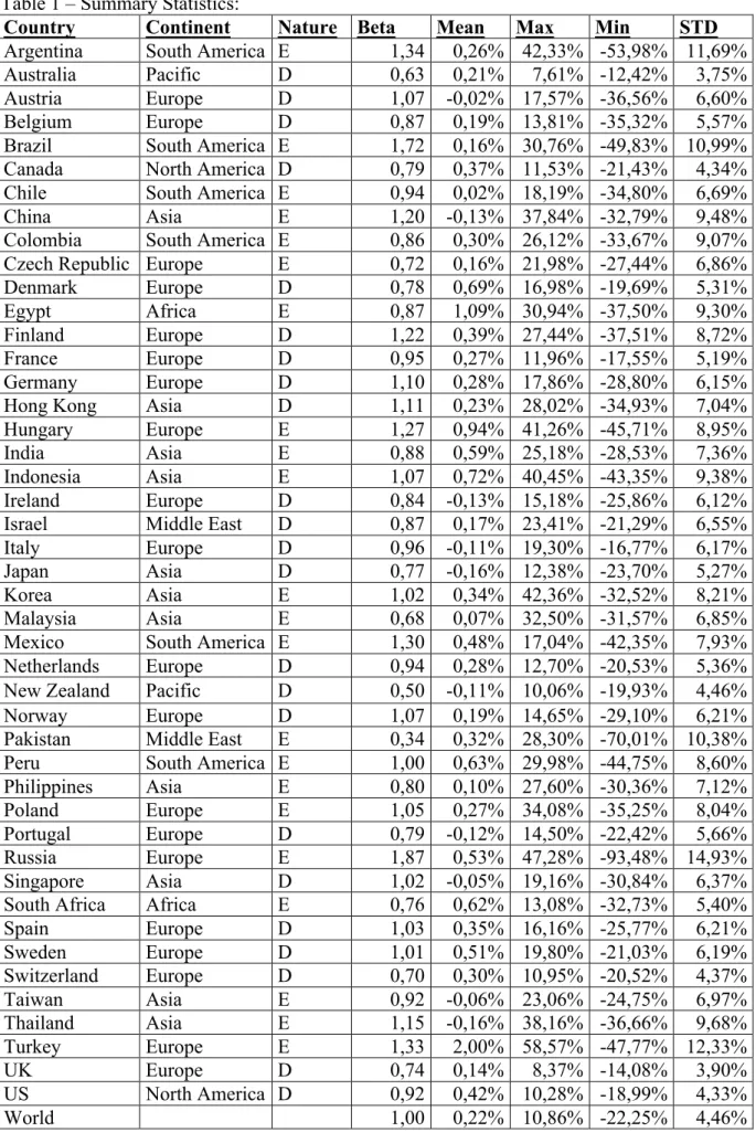
Table 1 – Summary Statistics:
Country Continent Nature Beta Mean Max Min STD Argentina South America E 1,34 0,26% 42,33% -53,98% 11,69%
Australia Pacific D 0,63 0,21% 7,61% -12,42% 3,75%
Austria Europe D 1,07 -0,02% 17,57% -36,56% 6,60%
Belgium Europe D 0,87 0,19% 13,81% -35,32% 5,57%
Brazil South America E 1,72 0,16% 30,76% -49,83% 10,99% Canada North America D 0,79 0,37% 11,53% -21,43% 4,34%
Chile South America E 0,94 0,02% 18,19% -34,80% 6,69%
China Asia E 1,20 -0,13% 37,84% -32,79% 9,48%
Colombia South America E 0,86 0,30% 26,12% -33,67% 9,07% Czech Republic Europe E 0,72 0,16% 21,98% -27,44% 6,86%
Denmark Europe D 0,78 0,69% 16,98% -19,69% 5,31%
Egypt Africa E 0,87 1,09% 30,94% -37,50% 9,30%
Finland Europe D 1,22 0,39% 27,44% -37,51% 8,72%
France Europe D 0,95 0,27% 11,96% -17,55% 5,19%
Germany Europe D 1,10 0,28% 17,86% -28,80% 6,15%
Hong Kong Asia D 1,11 0,23% 28,02% -34,93% 7,04%
Hungary Europe E 1,27 0,94% 41,26% -45,71% 8,95%
India Asia E 0,88 0,59% 25,18% -28,53% 7,36%
Indonesia Asia E 1,07 0,72% 40,45% -43,35% 9,38%
Ireland Europe D 0,84 -0,13% 15,18% -25,86% 6,12%
Israel Middle East D 0,87 0,17% 23,41% -21,29% 6,55%
Italy Europe D 0,96 -0,11% 19,30% -16,77% 6,17%
Japan Asia D 0,77 -0,16% 12,38% -23,70% 5,27%
Korea Asia E 1,02 0,34% 42,36% -32,52% 8,21%
Malaysia Asia E 0,68 0,07% 32,50% -31,57% 6,85%
Mexico South America E 1,30 0,48% 17,04% -42,35% 7,93%
Netherlands Europe D 0,94 0,28% 12,70% -20,53% 5,36%
New Zealand Pacific D 0,50 -0,11% 10,06% -19,93% 4,46%
Norway Europe D 1,07 0,19% 14,65% -29,10% 6,21%
Pakistan Middle East E 0,34 0,32% 28,30% -70,01% 10,38%
Peru South America E 1,00 0,63% 29,98% -44,75% 8,60%
Philippines Asia E 0,80 0,10% 27,60% -30,36% 7,12%
Poland Europe E 1,05 0,27% 34,08% -35,25% 8,04%
Portugal Europe D 0,79 -0,12% 14,50% -22,42% 5,66%
Russia Europe E 1,87 0,53% 47,28% -93,48% 14,93%
Singapore Asia D 1,02 -0,05% 19,16% -30,84% 6,37%
South Africa Africa E 0,76 0,62% 13,08% -32,73% 5,40%
Spain Europe D 1,03 0,35% 16,16% -25,77% 6,21% Sweden Europe D 1,01 0,51% 19,80% -21,03% 6,19% Switzerland Europe D 0,70 0,30% 10,95% -20,52% 4,37% Taiwan Asia E 0,92 -0,06% 23,06% -24,75% 6,97% Thailand Asia E 1,15 -0,16% 38,16% -36,66% 9,68% Turkey Europe E 1,33 2,00% 58,57% -47,77% 12,33% UK Europe D 0,74 0,14% 8,37% -14,08% 3,90% US North America D 0,92 0,42% 10,28% -18,99% 4,33% World 1,00 0,22% 10,86% -22,25% 4,46%
Table 1 reports summary statistics on the World index (MSCI), 23 developed markets and 22 emerging markets. The table includes: the country, its continent and nature, Emerging (E) or Developed (D), country betas, calculated with respect to the World index using Equation (2), monthly mean return, monthly minimum and maximum returns as well as the monthly standard deviation in returns over the January 1995 to May 2017 period.
Interestingly, from this data you can quickly notice that the country with the smallest standard deviation in monthly returns, Australia with 3,75%, also possesses the smallest minimum returns in a single month, -12,42%, as well as the smallest maximum return in a single month, 7,61%, over the full sample. On the other hand, the country with the largest standard deviation is Russia, with 14,93%, who also possesses the largest loss in a single month of -93,48%. However, Russia does not hold the largest maximum return in a single month, this is Turkey with 58,57%. Turkey also holds the largest average return at 2,00% whilst Japan and Thailand jointly experience the lowest average returns at -0,16%. Not surprisingly, and in-line with this data Australia’s returns range was merely 20,04% over the entire sample while Russia’s returns have a range of 140,76% demonstrating the contrasting stability of the different markets especially in the regard to emerging and developed markets. This higher volatility in emerging markets compared to developed markets is further confirmed when looking at the average range of returns in developed and emerging markets where developed markets have an average return range of 39,77%, whilst emerging markets have an average return range of 73,49%. Finally, the most important variable, for the purpose of this paper, are the beta values who range from 0,34 in Pakistan to 1,87 in Russia.
Data Reliability and Limitations:
The gathered data is very robust since firstly, the index price data is gathered from Bloomberg and only MSCI Indices are used, ensuring that each market’s prices are calculated using the same methodology, free-float weighted equity indices. Secondly, the US Treasury
bond rates are obtained from the Federal Reserve which is a reliable and prevalent source in the existing literature. In general, this means that the collected raw data can be deemed to be reliable, firstly due to the sources, but also due to the initial results. After the first regression the individual country beta values are calculated and are, as to be expected, within a range of +/- 1 of the value of 1. Thirdly, the sample size is sufficiently large in comparison to the existing literature, where often a data range of 20-30 years is used and this study examines just over 22 years of data. A larger sample period was considered, however, starting the sample period before January 1995 would decrease the sample size by at least 10 countries, most of which are emerging countries, as some MSCI market indices only launched in January of 1995. In order to keep a large sample of diversified markets and to keep a focus on emerging markets, the sample period was chosen to start in January 1995 rather than before. Additionally, the sample size in terms of the number of markets examined, 45, is very large compared to the existing literature, where studies often examine single countries or groups of 10-15 countries. Furthermore, the majority of existing literature focuses on examining markets of developed countries and less so on markets of emerging countries. This study, however, examines 45 countries evenly mixed between emerging and developed countries from across the globe, not only adding this to the existing literature, but moreover adding a global factor to the robustness of the final results.
Although the sample size is sufficiently large, the majority of developed markets in the sample originate from Europe, 15 out of 23 to be exact, almost two-thirds. As all these countries operate in the same economic market and all, with the exception of the UK and Switzerland, use the Euro, their markets are correlated to a certain extent and can cause a bias for the developed market sample. Additionally, this paper has made use of a standard 1-year rolling window OLS regression to calculate time-varying beta values for each individual market per month. This can be classified as a limitation, as papers such as Renzi-Ricci (2016) and Nieto et
al. (2014) compare and evaluate the best methodologies for moving averages and both conclude that the use of a Kalman filter is more accurate than the standard OLS method for longer period moving averages. Nevertheless, one can just as well argue that the use of the standard OLS method is sufficiently accurate in this case, because the Kalman filter is more accurate for time-varying moving window averages of more than one year and the time frame used in this paper is exactly one year. Last but not least, a further limitation to this paper could be considered the use of monthly data rather than daily data. In order to further improve the reliability of the results of this paper one can consider using daily rather than monthly data, as this would give an even more detailed and accurate insight of the risk-return relationship. However, this brings along the major challenge of adjusting the various data series for the varying non-trading days per country, which is especially difficult with such large variety of markets as used in this paper. Overall, when considering the sample size, the sample period, the used methodology, as well as the robustness check done to confirm the final results, the data and results can be considered reliable even when taking into consideration the limitations of this paper.
Empirical Evidence:
In the first stage the country betas were computed as per Equation 2, these are presented in Table 1. The second stage of the methodology proceeds to test the unconditional relationship between beta and returns with constant betas in Equation (3). The test for the unconditional and conditional relationship is conducted by estimating cross-sectional regressions for each month and ultimately taking the average of the 268 regression estimates and computing the t-statistic for each mean coefficient. We first test the unconditional relationship for all countries in the sample before splitting the sample up between emerging and developed countries and testing the relationship for each sub-sample before moving on to the conditional relationship.
Table 2: Tests of unconditional beta and return relationship
Table 2 reports the mean result of 𝛾), the slope, of the stage two monthly cross-sectional regressions for the full sample, and both sub-samples of emerging and developed countries, taking into account the country betas calculated in the first stage. The t statistic values (in parentheses) are tested according to Fama and MacBeth (1973), testing whether the mean coefficient value is equal to zero. The asterisk (*) represents the values that are significant at 5% for a two-tailed test.
The results show that all 𝛾) values are not significant at the 5% level and thus we can’t reject, with a considerable amount of confidence, the null hypotheses that 𝛾) is equal to 0. These
results indicate with 95% confidence that there is no significant, unconditional, relationship between beta and return for both the full sample, as well as, the emerging market and developed market sub-samples. This is in-line with the original studies of Fama and French (1992, 1996), as well as, other studies from this time including Ferson and Harvey (1994), Jagadeesh (1992) and Strong and Xu (1997). As mentioned, the dominant conclusions in the existing literature, finds no significant unconditional relationship, which these results support, however, it does contradict a hand-full of studies that do find a significantly positive unconditional relationship such as Heston et al. (1999) and the original studies of Fama and Macbeth (1973) and Black et al. (1972).
As discussed in the methodology, Pettengill et al. (1995, 2002) argue that when we differentiate between and down-markets there should be a positive market premium in up-markets and a negative premium in down-up-markets. This implies a positive conditional beta and return relationship in up-markets and a negative conditional relationship in down-markets. To test this conditional relationship, the data is cross-sectionally regressed using a dummy variable as in Equation 4.
Full Sample Emerging Developed
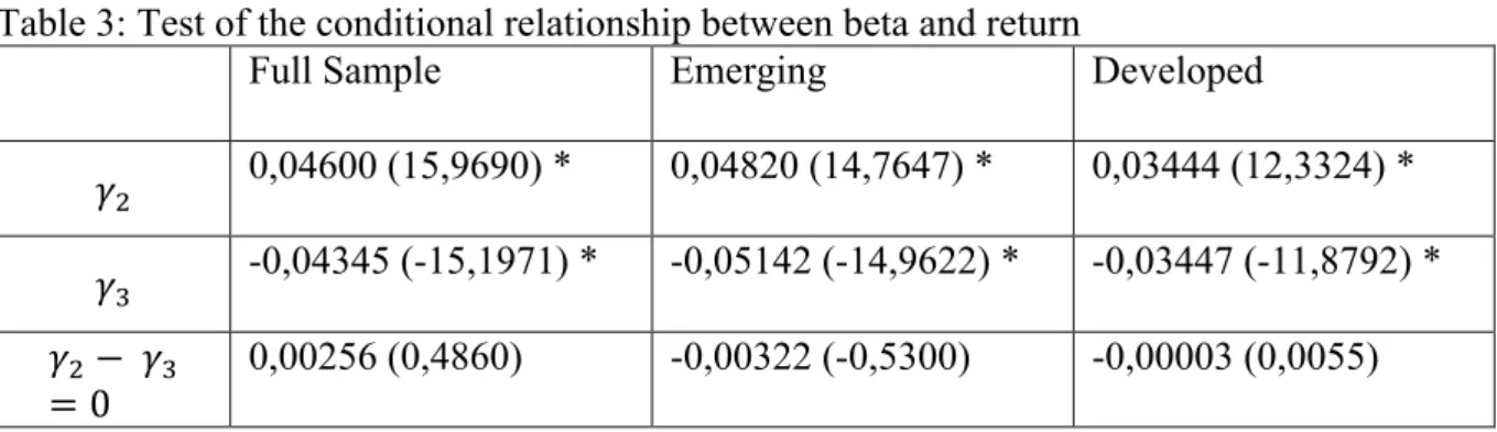
Table 3: Test of the conditional relationship between beta and return
Full Sample Emerging Developed
𝛾= 0,04600 (15,9690) * 0,04820 (14,7647) * 0,03444 (12,3324) *
𝛾@ -0,04345 (-15,1971) * -0,05142 (-14,9622) * -0,03447 (-11,8792) * 𝛾=− 𝛾@
= 0
0,00256 (0,4860) -0,00322 (-0,5300) -0,00003 (0,0055)
Table 3 reports the mean monthly returns in up-markets, 𝛾=, positive market returns, and mean monthly returns in down-markets, 𝛾@, negative market returns, for the whole sample, and both
sub-samples of emerging and developed countries, taking into account the country betas calculated in the first stage. We also add the t-statistic for Equation 6. Again the t-statistic values (in parentheses) are tested, this time one tailed, according to Fama and MacBeth (1973) testing whether the mean coefficient values of 𝛾= and 𝛾@ are significantly positive and negative, respectively. The asterisk (*) represents the values that are significant at 5% for a one-tailed test for 𝛾= and 𝛾@ and a two-tailed test for Equation 6.
The results and the t-statistic values found for 𝛾= and 𝛾@, for the full sample, as well as, the two sub-samples are all significant at 5%, meaning we reject the null hypothesis that 𝛾= or 𝛾@ are equal to zero with a 90% confidence level. More interestingly however 𝛾= and 𝛾@ for all three samples are even significant at a 0,05% level and we can reject the null hypothesis that 𝛾= and 𝛾@ are equal to zero with 99,9% confidence. Overall these results in regards to the conditions required for a conditional beta and return relationship are very positive and confirm the risk premiums with a high level of confidence. This indicates that there is a significant negative, as well as, a significant positive conditional relationship between beta and return during down-markets and up-markets, respectively, for all considered samples and that the recorded coefficients are good approximations of reality.
However, as argued by Pettengill et al. (1995) in order for the conditional relationship to hold there should not only be positive premiums in up-markets and negative premiums in down-markets, but moreover these premiums should be symmetrical. The final row, examines the symmetrical relationship between 𝛾= and 𝛾@ and demonstrates that, for the full sample and
zero. In other words, in the full sample and both sub-samples there is a good possibility of the existence of a symmetrical relationship between 𝛾= and 𝛾@. The null hypothesis here cannot be rejected with 95% confidence indicating that the calculated premiums have a very high likelihood to be symmetrical and that there is significant evidence of a conditional relationship between beta and return. These results are in-line with the recent existing literature, where Fletcher (1997; 2000), Morelli (2011), Elsas et al. (2003), and Girard et al. (2001), among others, also find significant conditional relationships after differentiating between up- and down-markets.
Robustness Check with Time-Varying Betas
Having established the first set of results with constant betas for the individual
markets, the unconditional and conditional relationship regressions are ran again utilizing the newly calculated 1-year time-varying betas. These betas will be a better estimation of the individual beta situation in each market for each month as they merely consider the recent, 1-year return history rather than the return history of the full sample period of 22 1-years. As a result of using a 1-year time varying beta values, the mean coefficient values are this time based on 257 regressions. This will thus complement the previous results and confirm or disprove the findings according to the original methodology presented by Pettengill et al (1995).
Table 4: Tests of unconditional beta and return relationship with 1-year time-varying betas.
Full Sample Emerging Developed
𝛾) -0,00192 (-0,6040) -0,00107 (-0,3259) -0,00466 (-1,4078)
Table 4 reports the mean results for 𝛾), the slope, of the stage two monthly cross-sectional regressions for the full sample, and both sub-samples of emerging and developed countries, taking into account the 1-year time-varying betas. The t-statistic values (in parentheses) are tested according to Fama and MacBeth (1973), testing whether the mean coefficient value is equal to zero. The asterisk (*) represents the values that are significant at 5% for a two-tailed test.
The results of the unconditional relationship robustness check show that the 𝛾) values are not significant at the 5% level. Moreover the 𝛾) values for the developed sample are only significant at the 10% level whilst the full and emerging samples are not even significant at a 50% level of a two-tailed test. This means that we can’t reject the null hypotheses that 𝛾) is equal to zero and thus can’t confirm with 95% confidence the existence of an unconditional relationship. An interesting observation from this robustness check is that when using 1-year time-varying betas the evidence of an unconditional relationship becomes slightly stronger, yet remains insignificant, compared to the evidence when merely using constant betas.
Nonetheless, these results again indicate that there is no significant unconditional relationship between beta and return for both the full sample, as well as, the emerging market and developed market sub-samples. This is again in-line with the original studies of Fama and French (1992, 1996), as well as, other studies from this time including Ferson and Harvey (1994), Jagadeesh (1992) and Strong and Xu (1997). As mentioned, the dominant conclusions in the existing literature, finds no significant unconditional relationship, which these results support, however, it does contradict a hand-full of studies that do find a significantly positive unconditional relationship such as Heston et al. (1999), Fama and Macbeth (1973) and Black et al. (1972). The originally calculated results for unconditional relationship are thus confirmed when using the 1-year time-varying betas, adding to the robustness and reliability of the original results.
Again, to test the conditional relationship we cross-sectionally regress the data using a dummy variable in Equation 4, however this time we again use the calculated 1-year time-varying betas to check the robustness of the original results.
Table 5: Test of the conditional relationship between beta and return with 1 year time-varying betas.
Full Sample Emerging Developed
𝛾= 0,03790 (14,9293) * 0,04390 (7,7334) * 0,02984 (13,9455) * 𝛾@ -0,04232 (-18,1679) * -0,04428 (-11,0591) * -0,04052 (-15,2696) * 𝛾= − 𝛾@ = 0 -0,00442 (-1,1154) -0,00039 (-0,0510) -0,01068 (-2,6533) * Table 5 reports the mean monthly returns in up-markets, 𝛾=, positive market returns, and mean monthly returns in down-markets, 𝛾@, negative market returns, for the whole sample, and both sub-samples of emerging and developed countries, taking into account the 1-year time-varying betas. We also add the t-statistic for Equation 6. Again the t-statistic values (in parentheses) are tested, this time one tailed, according to Fama and MacBeth (1973) testing whether the mean coefficient values of 𝛾= and 𝛾@ are significantly positive and negative, respectively. The asterisk (*) represents the values that are significant at 5% for a one-tailed test for 𝛾= and 𝛾@ and a two-tailed test for Equation 6.
The results and the t-statistic values found for 𝛾= and 𝛾@, for the full sample, as well as, the two sub-samples, are significant at 5% meaning we reject the null hypothesis that 𝛾= or 𝛾@ is equal to zero at 90% confidence. More interestingly however for each sample the conditional relationship between risk and return is slightly more significant during down-markets compared to up-markets i.e. the value for 𝛾@ is more significant compared to the 𝛾= value for all respective samples. For all samples the coefficient values of 𝛾= and 𝛾@ are significant at a 0,05% level and we can reject that 𝛾= and 𝛾@ is equal to zero with a 99,9% confidence level.
Also the results for the conditional relationship between beta and return, taking into account 1-year time-varying betas, are very good in regards to finding the conditional relationship and again confirm the risk premiums with a high level of confidence. This indicates that there is a significant negative, as well as, a significant positive relationship between beta and return during down-markets and up-markets, respectively, for all considered samples. Therefore, it can be concluded that the recorded coefficients are good approximations of reality also when considering time-varying betas.
However, again these results on their own don’t guarantee the existence of a conditional risk-return relationship and the final row therefore examines the symmetrical relationship between 𝛾= and 𝛾@, which is a crucial condition for the conditional relationship to exist. The results demonstrate that, for the full sample and the emerging market sub-sample, we can’t reject, with 95% confidence, the null hypothesis at 5% significance that 𝛾=− 𝛾@ equals zero. However, for the developed market sub-sample the null hypothesis can be rejected with 95% confidence at 5% significance, and can even be rejected at a 99% confidence level. This in essence means that we find a large possibility of the required symmetrical relationship between 𝛾= and 𝛾@ for the full sample and the emerging market sub-sample, but not for the developed market sub-sample. These results indicate that there is a lack of the symmetrical condition applicable for the developed market and thus the conditional relationship does not hold for this sample, whereas the relationship does hold for the full sample and the emerging market sub-sample. As the results indicate that the calculated premiums have a very high likelihood to be symmetrical for the full sample and that the result of the developed market sample might be limited due to possible bias created by the large number of European countries, it’s still possible to deduce that there is significant evidence of a conditional relationship between beta and return. The existing literature has not experimented much with time-varying betas, however, the found results are generally speaking in-line with the general results in the existing literature, where Fletcher (1997; 2000), Morelli (2011), Elsas et al. (2003) and Girard et al. (2001), among others, find significant conditional relationships.
Conclusions:
The risk-return discussion and theory is a main concept in the finance literature, and the notion that for higher risk, investors require a higher return is widely accepted, however, this does have its criticisms and doubts in the existing literature. The unconditional and conditional
relationships between beta and return are examined in a well-diversified sample of 45 countries, 22 emerging and 23 developed, over a sample period from January 1995 to May 2017. The unconditional and conditional relationships are initially examined over the whole sample and then divided into the emerging and developed market sub-samples.
For the unconditional relationship in the full sample as well as both sub-samples, no significant positive relationship is found. This is the case when following the original methodology as suggested by Pettengill et al. (1995) and is furthermore confirmed when checking the robustness of these results by taking into consideration, 1-year time-varying betas. These results demonstrate robustness and are in-line with the general findings and consensus of the existing literature in regards to the unconditional relationship between beta and return.
As argued by Pettengill et al. (1995), in order for the conditional relationship between beta and return to hold, the results between up- and down-markets have to be firstly, significantly positive in up-markets and significantly negative in down-markets, and secondly, they have to be symmetrical. The results based on purely following Pettengill et al. (1995) methodology are very positive and in-line with the existing literature, as a significant positive relationship in up-markets and significant negative relationship in down-markets is found. Moreover, the results of the symmetrical t-tests are insignificant and thus the null hypotheses cannot be rejected. In other words, the symmetrical tests conclude that there is a significantly large probability that the results of the relationship in up- and down-markets are indeed significant and have a good chance to be symmetrically opposite i.e. a significant conditional relationship is found. To test the robustness of these results again the process was repeated with 1-year time-varying beta values. The results remain relatively consistent and again a significant positive and negative relationship was found in up- and down-markets, respectively, for all samples. Also the symmetrical test’s null hypothesis cannot be rejected with any significance for the full sample and the emerging market sub-sample, however, the symmetrical relationship
can be rejected at a 5% significance level for the developed market sub-sample. The robustness test confirms the evidence and presence of a conditional relationship for the full and emerging market sample, but the developed market sample fails the robustness check. As mentioned previously, although the confidence levels slightly decreased when using the 1-year time-varying beta values over the constant beta values, the results remained very consistent and this paper can confirm the existence of a conditional relationship, regardless of the developing market sub-sample failing the robustness check.
This paper confirms the findings of a large section of the existing literature such as Fletcher (1997; 2000), Morelli (2011), Hodoshima (2000), Elsas et al. (2003) and Girard et al. (2001) who don’t find evidence of the unconditional risk-return relationship, however, when differentiating between up- and down markets they do find significant evidence of the conditional risk-return relationship. This paper not only confirms these exact results and agrees with the general consensus in the existing literature, but it adds the confirmation of these results in a large sample of emerging countries as well. The existing literature is largely focused on developed markets and thus this paper adds a global factor to the robustness of the results in the general literature, due to the large sample size and focus on both emerging and developing markets alike across all continents. Additionally, it also demonstrates the importance of considering the market state for the existence of a risk-return relationship, as the hypotheses of unconditional relationships are all rejected at the 5% significance level, whilst the conditional relationship hypotheses cannot be rejected at the 5% significance level and often not even at a 1% significance level.
The only real outlying result, as explained, could have occurred due to the limitation of the developed market sample having 15 of 23 countries originating from Europe which may have an associated bias due to them operating in the same economic market. Regardless, the overall results demonstrate that the conditional relationship consistently holds fully for the full
and emerging market samples and we can conclude and deduce that the risk- return relationship exists, when considering the market state i.e, the conditional relationship exists whilst the unconditional relationship doesn’t. This indicates that the results and coefficients of this paper are good approximations of reality and suggests that beta is useful and accurate tool to explain cross-sectional differences between country index returns when taking into account the nature of the current market.
The data, results and conclusions of this paper are very robust, however, to further improve the reliability of the results daily data rather than monthly data can be used and a slight alteration can be made to the methodology on how to calculate the time-varying betas. Rather than using a basic OLS 1-year rolling window, the Kalman filter methodology can be used. Overall however, this is only a small improvement to increase the precision and the robustness of the obtained results. A slightly more significant limitation would be the fact that the methodology only examines the risk-return relationship contemporaneously and doesn’t take into account the lagged effect of up and down markets on the next periods return. Finally, to extend this research, each market index can be examined in more detail itself, looking at the risk return relationship of individual stocks within the market indices and examine the un- and conditional relationship there to get a more detailed look at the risk-return relationships within individual markets. Additionally, it is possible to test the forecasting power of the conditional relationship between beta and returns, similar to Verma (2011), as another extension to this paper.
References
Black, F. (1972). Capital Market Equilibrium with Restricted Borrowing. The Journal of Business, 45, 444-455.
Black, F., Jensen, M., & Scholes, M. (1972). The Capital Asset Pricing Model: Some Empirical Tests. Studies in the Theory of Capital Markets, 79-121.
Daniel, K., & Titman, S. (1997). Evidence on the Characteristics of Cross Sectional Variation in Stock Returns. The Journal of Finance, 52, 1-33.
Elsas, R., El-Shaer, M., & Theissen, E. (2003). Beta and Return Revisited Evidence from the Germand Stock Market. Journal of International Financial Markets, Institutions and Money, 13, 1-18.
Fama, E. F., & French, K. R. (1992). The Cross-Section of Expected Stock Returns. The Journal of Finance, 47, 427-465.
Fama, E., & French, K. (1996). The CAPM is Wanted, Dead or Alive. The Journal of Finance, 51, 1947-1958.
Fama, E., & MacBeth, J. (1973). Risk, Return, and Equilibrium: Empirical Tests. The Journal of Political Economy, 81, 607-636.
Ferson, W., & Harvey, C. (1991). The Variation of Economic Risk Premiums. The Journal of Political Economy, 99, 385-415.
Ferson, W., & Harvey, C. (1993). The Risk and Predictability of International Equity Returns. The Review of Financial Studies, 6, 527-566.
Ferson, W., & Harvey, C. (1994). Sources of Risk and Expected Returns in Global Equity Markets. Journal of Banking and Finance, 18, 775-803.
Fletcher, J. (1997). An Examination of the Cross-Sectional Relationship of Beta and Return: UK Evidence. Journal of Economics and Business, 41, 211-221.
Fletcher, J. (2000). On the Conditional Relationship between Beta and Return in International Stock Returns. International Review of Financial Analysis, 9, 235-245.
Girard, E., Rahman, H., & Zaher, T. (2001). Intertemporal Risk-Return Relationship in the Asian Markets around the Asian Crisis. Financial Services Review, 10, 249-272. Harvey, C. (1989). Time-Varying Conditional Covariances in Tests of Asset Pricing Models.
Journal of Financial Economics, 24, 289-317.
Heston, S., Rouwenhorst, K., & Wessels, R. (1999). The Role of Beta and Size in the Cross-Section of European Stock Returns. European Financial Management, 5, 9-27. Hodoshima, J., Garza-Gómez, X., & Kunimura, M. (2000). Cross-Sectional Regression
Analysis of Return and Beta in Japan. Journal of Business and Economics, 52, 515-533.
Jegadeesh, N. (1992). Does Market Risk Really Explain the Size Effect? The Journal of Financial and Quantitative Analysis, 27, 337-351.
Korajczyk, R., & Viallet, C. (1989). An Empirical Investigation of International Asset Pricing. The Review of Financial Studies, 2, 553-585.
Lintner, J. (1965). The Valuation of Risk Assets and the Selection of Risky Investments in Stock Portfolios and Capital Budgets. The Review of Economics and Statistics, 47, 13-37.
Mollik, A., & Bepari, M. (2015). Risk-Return Trade-off in Emerging Markets: Evidence from Dhaka Stock Exchange Bangladesh. Australasian Accounting, Business and Finance Journal, 9, 71-88.
Morelli, D. (2011). Joint Conditionality in Testing the Beta-Return Relationship: Evidence based on the UK Stock Market. Journal of International Financial Markets,
Mossin, J. (1966). Equilibrium in a Capital Asset Market. Econometrica, 34, 768-783. Nieto, B., Orbe, S., & Zarraga, A. (2014). Time-Varying Market Beta: Does the Estimation
Methodology matter? Statistics and Operations Research Transactions, 38, 13-42. Pettengill, G., Sundaram, S., & Mathur, I. (1995). The Conditional Relation between Beta and
Returns. The Journal of Financial and Quantitative Analysis, 30, 101-116.
Pettengill, G., Sundaram, S., & Mathur, I. (2002). Payment for Risk: Constant Beta vs. Dual-Beta Models. The Financial Review, 37, 123-136.
Renzi-Ricci, G. (2016). Estimating Equity Betas: What can a Time-Varying Approach Add? NERA Economic Consulting, 1-9.
Sehgal, S., & Garg, V. (2016). Cross-Sectional Volatility and Stock Returns: Evidence for Emerging Markets. The Journal for Decision Makers, 41, 234-246.
Sharpe, W. (1964). Capital Asset Prices: A Theory of Market Equilibrium under Conditions of Risk. The Journal of Finance, 19, 425-442.
Strong, N., & Xu, X. G. (1997). Explaining the Cross-Section of UK Expected Stock Returns. British Accounting Review, 29, 1-23.
Verma, R. (2011). Testing Forecasting Power of the Conditional Relationship between Beta and Return. The Journal of Risk Finance, 12, 69-77.