Nonlinear Time-Varying Parameter Estimation from Noisy Measurements
Milca de Freitas Coelho;[email protected]University of Beira Interior
K. Bousson - [email protected]
LAETA-UBI/AeroG & Department of Aerospace Sciences, Laboratory of Avionics and Control, Faculty of Engineering University of Beira Interior
Kawser Ahmed - [email protected]
LAETA-UBI/AeroG & Department of Aerospace Sciences, Laboratory of Avionics and Control, Faculty of Engineering University of Beira Interior
Abstract
Online parameter estimation for time-varying systems is a fundamental part of adaptive control, real-time system monitoring and prediction. A well-known framework for dealing with such a task is the Kalman filtering. Meanwhile Kalman filtering may be cumbersome for some time-critical systems and inappropriate for systems whose stochastic characteristics are not Gaussian. To overcome these shortcomings, a parameter estimation algorithm devised from Sutton’s dynamic learning rate techniques and based on a learning window and forgetting factor criterion has been used. In doing so, the proposed algorithm avoids the need for heuristic choices of the initial conditions and noise covariance matrices required by the Kalman filtering. The performance of the proposed method is demonstrated successfully on a lateral-directional flight dynamics parameter estimation process for an unmanned aerial vehicle through computational simulation.
Keywords
Nonlinear Time-Varying Parameter Estimation
from Noisy Measurements
1 Introduction
Parameter estimation is one of the fundamental tools for dealing with time-varying systems, mainly in system control, filtering, identification and prediction. For instance, in aerospace industries, due to the limitation in the size of wind tunnels and to the size of the aircraft prototypes to be used in these wind tunnels, aerodynamic parameters may be estimated from flight testing data [3]. It is more appropriate to estimate these parameters along with the acquisition of the necessary data during flight tests instead of doing it off-line as is often done. The interest of estimating dynamical system parameters on-line is manifold. For instance, the control strategy may be improved by the possibility of using the estimated parameters for predicting some state or output variables, adapting the control parameters according to these predictions, or estimating the performances of the underlying dynamic system so that they can be improved efficiently.
There are two main groups of methods for coping with parameter identification: the gradient descent and the Kalman filtering based methods [1,4]. Meanwhile, the work of Sutton [8,9] with linear networks sheds the light on the relationship between these two groups, and it can be shown that the problem of sequentially updating the learning rates in gradient descent algorithms and that of updating the system and process noise covariance matrices in Kalman filtering are equivalent. However, it is known that the application of the Kalman filtering algorithm may be inefficient if the stochastic behavior of the system is not well understood, mainly if the noise covariance matrices are wrongly chosen. Therefore, Sutton [9] has proposed a gradient descent method for updating the Kalman gain, which is void of any special prior knowledge of the process noise covariance matrix, and at the same time reducing the computational time and increasing the efficiency of the filtering process.
The present paper extends Sutton’s filtering algorithm to the case of nonlinear systems with parameters that are possibly time-varying. For such systems, one of the approaches is to estimate the model parameters at time t, taking into account only the last L measurements on the system, iterating from the value of the parameter at t-1. In the context of incremental least square methods, Bertsekas [2] has given a solution to a problem which is equivalent to the one we intend to solve, but from the standpoint of the Kalman filtering. The purpose of the present paper is to propose a solution based on the nonlinear extension to the Sutton linear filtering approach keeping its advantages over the Kalman filtering, and to give an application to the estimation of aircraft aerodynamic parameters during flight tests.
2 Problem Statement
In the discrete-time domain, the system model may be represented by the equation:
k k k
k
x
v
y
(
,
)
(1)where xk, yk, k, and vk are respectively the model input, the model output, the model parameter, and the white noise at discrete time k, and being a nonlinear function of its arguments. The model parameter k will be referred to as the parameter vector in the sequel.
It is assumed that there are means to measure the output vector
y
k on-line for any setting of the input vectorx
k across time. The measurements are taken according to a certain time-period t at times:...
,
.
...,
,
.
2
,
,
1 0 2 0 0 0t
t
t
t
t
t
t
t
n
t
t
n
The problem to be solved in the present paper is to find the parameter vector on-line at each discrete time ti
(
i
1
),
along with the data acquisition process on the system, such that the predictions across-time of the output vector be as close as possible to its corresponding actual measurements.3 Solution Proposal
In the case of linear time-invariant systems, the parameter k is constant (k = ), and the cost function which is usually adopted for identifying that parameter with measurements up to time t is of least square type:
2 0
)
,
(
)
(
t k k kx
y
J
(2)Furthermore, in the linear case, (Eq. 1) is expressed as:
k k T k k
x
v
y
(3)where (.)T is the transposition operation. In its simplest form, the gradient descent algorithm for updating the parameter vector is expressed by the following equation:
k k T k k k k
ˆ
(
y
x
ˆ
)
x
ˆ
1
(4)where
ˆ
k denote the estimates of
kand
a constant learning rate. To improve that scheme it is better to associate a variable learning rate with each component of the parameter vector as done for instance by Sutton [8,9]:) ( ) ( ) ( ) ( 1
ˆ
(
ˆ
)
ˆ
i k k T k k i k i k i k
y
x
x
(5)where the upper script (i) indicates the ith component of the corresponding variable. It is clear that the Kalman filtering algorithm is also an example of a variable learning rate algorithm with: k k k T k k k k k
x
Q
P
x
R
Q
P
)
(
1
(6)where Pk and Qk are respectively the update matrix and the noise covariance matrix, and
}.
{
kT kk
E
v
v
Due to the complexity encountered in the applications of the Kalman filtering when probabilistic knowledge about the system is not available, Sutton devised filtering techniques [8,9], for linear time-invariant systems, which are void of probabilistic information, and which have performances comparable to those of the Kalman filtering methods. Sutton filtering techniques consist in approximating matrix P+Q in (Eq. 6) with a diagonal matrix whose ith diagonal element is given by:
)
exp(
(i)ii
p
(7)where (i) is updated by the least mean square rule devised such that the learning rate for each model parameter is updated sequentially. The Sutton filtering algorithm is dedicated to linear time-invariant systems, that is, systems satisfying (Eq. 3). In the context of nonlinear time-varying systems, the cost function to be minimized is no longer given by (Eq. 2) but by a functional which accounts for the variability of the parameter across time. Assuming the parameter variation to be smooth, it can be shown that the minimization of the following time-dependent cost function allows to track the parameter [2]:
2 1 1 1
)
(
)
(
,
)
(
)
(
t L t k t k k k t t t t T t t t tH
y
x
J
(8)where t is the current time, Ht is a time-varying positive definite matrix, L is the learning window length, and is a scalar forgetting factor with:
1
0
(9)The nonlinear counterpart of the Sutton’s filtering may be based on the linearization of (Eq. 1) about the current estimate
ˆ
k of the parameter vector assuming function
to be derivable with respect to its second argument (the parameter vector). Therefore, with respect to the criterion stated in (Eq. 8), the extension of the Sutton’s filtering technique [8,9] to nonlinear time-varying systems gives:k
ˆ
1 0
;H
0
0
(10)
,
0
,
1
,...,
1
,
)
ˆ
(
1 1 1 1
K
y
y
P
tH
t t tt
L
t t L k t L k t t t
(11)
(
,
)
(
,
)
,
0
,
1
,...,
,
)
,
(
L
t
x
P
x
x
P
K
t t t T t t t t t t
(12)
(
,
)
,
0
,
1
,...,
1
,
)
,
(
1
H
x
x
t
L
H
t
t t
t t
t T (13) L k
ˆ
1
(14)where
y
t is the measurement vector at t,y
ˆ
t
(
x
t,
t)
the measurement estimate,)
,
(
x
t
t
is the gradient of
(
x
t,
)
with respect to
at
t,
and Pt is defined as a diagonal matrix whose ith diagonal element is given by (Eq. 7) for t = 1, ..., L, with for each i and t:
(
,
)
,
0
,
1
,...
1
0
) ( ) ( ) ( ) ( 1 ) ( 0L
t
h
x
t t ti i t i t i t i
(15)where is a small positive parameter,
t is the error:
t
y
t
(
x
t,
t),
(
,
)
) ( t t ix
isthe ith component of the gradient
(
,
)
t t
x
, and (i) th
is defined as:
1
,...,
1
,
0
,
)
,
(
1
0
) ( ) ( ) ( ) ( ) ( ) ( 0L
t
x
K
K
h
h
h
t t i i t t i t i t i t i
(16) with (i) tK
being the ith component ofK
t,
and (a)+ the positive part of the real a, that is:).
,
0
( a
max
a
4 Numerical Application
Consideration is given here to an application to stability and control derivative estimation in a lateral-directional flight [3,6,7]. The angle of attack is assumed to be nearly equal to zero, and the altitude may suffer some low frequency and low amplitude oscillations about a given constant value. With respect to a moving flat earth (assumed) and non-rotating reference frame translating with the local air mass, the equations describing the dynamics of an aircraft in the horizontal plane, when the aircraft is seen as a rigid body with no idle thrust, can be written as follows [5]:
m
D
T
V
C
V
c
S
h
qr
I
pq
I
I
p
I
r
I
C
V
c
S
h
pq
I
qr
I
I
r
I
p
I
sin
mg
C
SV
h
r
mV
n xz x y xz z l xz y z xz x y
2 2 2)
(
2
1
)
(
)
(
2
1
)
(
.
)
(
2
1
)
(
(17)where
C ,
yC
l andC
n are respectively the side-force coefficient, rolling moment coefficient and yawing moment coefficient, and defined as:
r n a n nr np n n r l a l lr lp l l r y a y y y r a r a r aC
C
V
rb
C
V
pb
C
C
C
C
C
V
rb
C
V
pb
C
C
C
C
C
C
C
(18)For a lateral-directional flight with constant altitude and nearly zero pitch angle, the Euler attitude dynamics equations reduce to the following simple equations:
sin
cos
tan
p
q
r
q
r
(19)
T
m
T
T
T
m ax
1
(
)
(20)Nomenclature
V
: aircraft speed, T : thrust, : yaw angle,
: bank angle,h
: flight altitude,
(h
)
: air density at altitudeh
,S : wing reference area, m : aircraft mass,
g : acceleration of the gravity, p, q, r : roll rate, pitch rate, yaw rate,
D : drag, : sideslip angle,
r a r a r a n n nr np n l l lr lp l y y yC
C
C
C
C
C
C
C
C
C
C
C
C
,
,
,
,
,
,
,
,
,
,
,
,
: stability and control derivatives
c
: mean chord length,b : wing span,
Ix,Iy,Iz : moment of inertia about the longitudinal, lateral and vertical axes of the aircraft,
Ixz : product of inertia in the (x,z)-plane,
: time constant of the propulsion system (when the throttle is activated), this parameter depends on the altitude h, the aircraft speed V, and the position of the throttle .
: position of the throttle expressed as a number in interval [0, 1],
Tmax : maximal thrust available, : specific fuel consumption.
The air density (h) at altitude h is given as:
5 4.256060537 0 0(1 2.2558 10
)
,
11000
( )
0.2971
exp 0.0001576939(11000
) ,
11000
20000
h
if h
m
h
h
if
h
m
(21) where
0
1
.
225
kg
/
m
3.
The state, control and parameter vectors of the aforementioned model are given respectively by (Eq. 22, 23, 24) below:
Tx
p r V T m
(22)
T r au
(23)
T n n nr np n l l lr lp l y y yC
aC
rC
C
C
C
aC
rC
C
C
C
aC
rC
(24)where [.]T denotes the vector transposition operator. So, the system of equations (Eq. 17, 19, 20) can be written as:
( , , )
noise
x
f x u
(25)The problem here consists in estimating the parameter vector
as defined in (Eq. 24). The experiments have been done with an unmanned aerial vehicle (UAV) model. The data related to the specific model used for the application of the method are:2 2 2 2 2 2 max 6 2
0.625
,
0.25 ,
2.5 ,
0.617
.
,
0.339
.
,
0.933
.
,
0.036
.
,
1254.4
,
9.8
/
,
100
,
3.381 10 ,
1 ,
0.8,
0.0303 0.0235
0.0659
,
0.5378.
x y z xz L L LS
m
c
m
b
m
I
kg m
I
kg m
I
kg m
I
kg m
T
N
g
m s
h
m
s
D
C
C
C
The initial conditions used for the simulation are:
0
0
0 ,
p
0r
0 0 00,
V
038
m s
/ ,
T
0820
N
,
m
055
kg
.
The model equation (Eq. 25) has been simulated (in the mean-square sense, assuming zero-mean noise) using the modified Euler scheme described below (or any other numerical integration scheme) where t denotes the integration stepsize:
1 1 1 1 1ˆ
ˆ
,
,
;
ˆ
.
ˆ
ˆ
ˆ
ˆ
,
,
;
.
2
n n n n n n n n n n n n n n ny
f x u
x
x
t y
t
y
f x
u
x
x
y
y
(26)It is obvious that the expression
x
ˆ
n1
x
ˆ
n
(
t
2).
y
n1
y
ˆ
n
that appears in (Eq. 26) may be written as an equivalent equation that has the form of (Eq. 1).The integration step size for the simulation has been taken constant and equal to
001
.
0
t
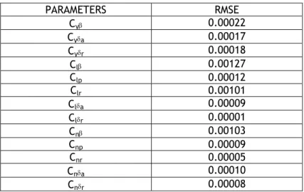
second. Disturbances in the rudder and the ailerons were applied to a known nonlinear model (hence, the stability derivatives were all known) to produce simulated data for the state responses of the aircraft. These data were then corrupted with 10% Gaussian random noise, which made the signal-to-noise ratio 10-to-1 for each simulated state measurement, but the ailerons and rudder input were assumed to be noise-free, which is close to reality. Based on these generated data, the identification of the stability derivatives were done from the simulation of the same aircraft model with the same rudder and ailerons disturbances and assuming the stability derivatives to be unknown. The window length L used in (Eq. 8) for the parameter estimation has been set toL
20
,
which means that the current parameter estimate is based on the last twenty measurements. The estimates of each stability derivative were computed along one-hour flight simulation and compared with the actual values. Table 1 below summarizes the root mean square errors (rmse) obtained from these comparisons for all the considered stability derivatives during a flight that lasted 300 seconds (6 minutes) using the 3-2-1-1 input forms. One may observe that the proposed method is actually an accurate nonlinear parametric estimator.Table 1: Root mean square error for the stability and control derivatives identification PARAMETERS RMSE Cy 0.00022 Cya 0.00017 Cyr 0.00018 Cl 0.00127 Clp 0.00012 Clr 0.00101 Cla 0.00009 Clr 0.00001 Cn 0.00103 Cnp 0.00009 Cnr 0.00005 Cna 0.00010 Cnr 0.00008
5 Conclusion
A method for online parameter estimation is presented for nonlinear time-varying uncertain systems for which the stochastic characteristics of the uncertainties are not known. An adaptive estimation procedure with variable learning rate is proposed and applied successfully on real-time stability and control derivative determination. Because the method is void of prior stochastic information about the model uncertainties and measurement noise, it may well be an alternative to existing nonlinear (and linear) recursive parameter estimation methods mainly when information about uncertainties related to the model and the measurements is unavailable. Future work will investigate the extension of the proposed method to nonlinear adaptive control of uncertain systems.
Acknowledgments
This research work was conducted in the Laboratory of Avionics and Control and supported by the Aeronautics and Astronautics Research Group (AeroG) of the Associated Laboratory for Energy, Transports and Aeronautics (LAETA).
References
[1] Y. Bar-Shalom and X.R. Li: Estimation and Tracking: Principles, Techniques and Software, Artech House, Boston, 1993.
[2] D. Bertsekas, "Incremental least square methods and the extended Kalman filter", Report
LIDS-P-2237, MIT, 1994.
[3] K. Bousson, "On-line aircraft stability derivatives estimation", Proceedings of SAE-World
Aviation Congress, September 10-14, 2001, Seattle. Paper 01WAC-8.
[4] A.H. Jazwinski: Stochastic Processes and Filtering Theory, Academic Press, 1970.
[5] Stevens B. L., F.L. Lewis: Aircraft Control and Simulation, 2nd Edition. Wiley-Interscience, Inc., 2003.
[6] R.F. Stengel, Flight Dynamics. Princeton University Press, 2004.
[7] Y. P. Sun, L.T. Wu, L.C. Liang, "Stability Derivatives Estimation of Unmanned Aerial Vehicle", Key Engineering Materials, Vols. 381-382, 2008, pp. 137-140.
[8] R. Sutton, "Adapting bias by gradient descent: An incremental version of delta-bar-delta",
Proceedings of the Tenth National Conference on Artificial Intelligence, MIT Press, 1992, pp.
171-176.
[9] R. Sutton, "Gain adaptation beats least squares?", Proceedings of the Seventh Yale