Blind channel algorithms based on the parafac decomposition of cumulant tensors: the single and multiuser cases

Signal Processing 88 (2008) 1382–1401

Blind channel identification algorithms based on the Parafac

decomposition of cumulant tensors: The single

and multiuser cases

Carlos Esteˆva˜o R. Fernandes

a,1

, Ge´rard Favier

a,

, Joa˜o Cesar M. Mota

b

a_{I3S Laboratory, University of Nice Sophia Antipolis (UNSA), CNRS, 2000 route des Lucioles, 06903 Sophia Antipolis, France} b_{Teleinformatics Engineering Department (DETI), Federal University of Ceara´ (UFC), Campus do Pici, 60455-760 Fortaleza, Brazil}

Received 21 June 2007; received in revised form 30 November 2007; accepted 6 December 2007 Available online 23 December 2007

Abstract

In this paper, we exploit the symmetry properties of 4th-order cumulants to develop new blind channel identification algorithms that utilize the parallel factor (Parafac) decomposition of cumulant tensors by solving a single-step (SS) least squares (LS) problem. We first consider the case of single-input single-output (SISO) finite impulse response (FIR) channels and then we extend the results to multiple-input multiple-output (MIMO) instantaneous mixtures. Our approach is based on 4th-order output cumulants only and it is shown to hold for certain underdetermined mixtures, i.e. systems with more sources than sensors. A simplified approach using a reduced-order tensor is also discussed. Computer simulations are provided to assess the performance of the proposed algorithms in both SISO and MIMO cases, comparing them to other existing solutions. Initialization and convergence issues are also addressed.

r2007 Elsevier B.V. All rights reserved.

Keywords:Channel identification; Parameter estimation; Tensor decomposition; Underdetermined linear mixtures

1. Introduction

In digital telecommunication systems, parametric channel modelling and estimation are of great importance. The knowledge of the channel model can be used to design equalizers to deconvolve the

received signals. Channel identification and equal-ization consist in the retrieval of unknown informa-tion about the transmission channel and source signals, respectively. In order to reach a desired quality of service, broadband wireless communica-tion systems classically perform channel identifica-tion and/or equalizaidentifica-tion using pilot symbols, i.e. training sequences composed of a priori known signals. This supervised approach introduces an overhead to the transmission system that may not be suitable for certain radio communication systems since it reduces the effective transmission rate. On the other hand, unsupervised (or ‘‘blind’’) ap-proaches take only the output signals into account

www.elsevier.com/locate/sigpro

0165-1684/$ - see front matterr2007 Elsevier B.V. All rights reserved. doi:10.1016/j.sigpro.2007.12.010

_{Corresponding author. Tel.: +33 492 942 736;} fax: +33 492 942 896.

E-mail addresses:cfernand@i3s.unice.fr (C.E.R. Fernandes), favier@i3s.unice.fr (G. Favier),

mota@deti.ufc.br (J.C.M. Mota).

with possibly somea priorihypothesis on the input signals.

High-order statistics (HOS) have been an im-portant research topic in diverse fields including data communication, speech and image processing and geophysical data processing. For stationary real signals, the second-order statistics (SOS) are not able to keep the phase information of anonminimum

phase system and, unless additional information about the input signal is known, the use of HOS is generally mandatory for blindly identifying finite impulse response (FIR) channels. The high-order spectra have the ability to preserve both magnitude and (nonminimum) phase information. Moreover, it is well known that all the cumulants of order greater than 2 vanish for Gaussian signals, which makes HOS-based identification methods insensitive to an additive Gaussian noise (cf. [1,2] and references therein). A vast amount of papers exist on this subject, proposing different methods that exploit high-order cumulants (cf. [3–5]among others).

Output cumulants of order higher than two can be viewed as tensors with a highly symmetrical structure [6]. Among the earliest works exploiting the cumulant symmetries with a tensor formalism, Cardoso introduced the concept of eigen-structure of 4th-order cumulant tensors [7,8]. He used the uniqueness property of the cumulant tensors as an advantage over singular value decomposition (SVD), but pre-whitening was needed. Later on, an extended Jacobi technique for approximate simultaneous diagonalization was proposed by Cardoso and Soloumiac in [9]. This latter paper introduced the JADE algorithm that uses second and 4th-order statistics to estimate an instantaneous multiple-input multiple-output (MIMO) channel in the context of blind beamforming. The joint diagonalization technique became very popular and has been used by Belouchrani et al. to propose the second-order blind identification (SOBI) algo-rithm [10], which uses a set of correlation matrices to identify stationary sources with different spectral contents, also in the context of instantaneous MIMO channels. On the other hand, the fourth-order system identification (FOSI) algorithm [11]

treats single-input single-output (SISO) FIR chan-nels and also involves an a priori transformation over the cumulant matrices, which is often a source of increased complexity and estimation errors. Important modifications of the technique proposed in[8]were provided by De Lathauwer et al. in[12], resorting to joint diagonalization techniques. More

recently, the joint diagonalization approach has been used in[13] to propose the ICAR algorithm, which exploits the redundancies in the 4th-order cumulant to estimate the mixture matrix, but only in the overdetermined case, i.e. the case of systems with more sensors than sources. The quadricovar-iance is also used by the FOOBI-type algorithms proposed in [14], making use of its column-wise Kronecker structure to estimate underdetermined mixtures (more sources than sensors).

Since the introduction of the independent compo-nent analysis (ICA) concept in the seminal paper by Comon [15], research efforts have been spent for generalizing simultaneous diagonalization criteria and establishing links with canonical tensor decom-positions (cf. [16,17] and references therein). For instance, in[18], De Lathauwer et. al reformulated the canonical decomposition of high-order tensors as a simultaneous generalized Schur decomposition. The Parafac analysis of aP-dimensional tensor with rank

Fconsists in the decomposition of the tensor into a sum ofFrank-one tensors, each one being written as an outer product of P vectors [19]. It is now well known that the blind identification of linear mixtures is closely related to the (simultaneous) diagonaliza-tion of symmetric cumulant tensors[20,21]. The key-point in the use of the Parafac decomposition is its uniqueness property, which can be ensured under simple conditions that are stated in the Kruskal Theorem[22]. Furthermore, canonical tensor decom-positions do not impose any kind of orthogonality constraints and the factorization of tensors composed of high-order output cumulants has the advantage of avoiding the so-called pre-whitening operation by fully exploiting the multidimensional nature of the cumulant tensor. Moreover, the tensor rank is not bounded by the tensor dimensions as it is the case for matrices, which conceptually allows for the blind identification of underdetermined mixtures. Actually, this problem has received a special attention from the signal processing community under different tensor approaches that include, among others, the decom-position ofquanticsin sums of powers of linear forms

[23]; the use of congruent transformation [24]

A formal relationship between Parafac decom-position and simultaneous matrix diagonalization has been established in [32] showing that the components of the tensor decomposition can be obtained from a simultaneous matrix diagonaliza-tion by congruence transformadiagonaliza-tion, leading to weaker uniqueness conditions. These ideas gave rise to the FOOBI algorithms [14], which are theoreti-cally able to identify a greater number of user channels for a given number of receive antennas. The approach used by the ICAR method [13] can also include the case of underdetermined mixtures, resorting to 6th- [33]or higher-order statistics[24]. These latter papers propose methods avoiding pre-whitening, but still breaking the problem into two optimization procedures, which remains necessary to extract the MIMO channel coefficients from an initial estimate based on an eigenvalue decomposi-tion (EVD).

Several algorithms propose solutions to fit aP th-order Parafac model. The well-known alternating least squares (ALS) algorithm iteratively minimizes, in an alternate way, P least squares (LS) cost functions. Our main focus in this paper is to exploit the redundancies of the factors of the 4th-order cumulant tensor decomposition in the minimization problem in order to develop new single-step (SS) LS Parafac-based Blind Channel Identification (SS-LS PBCI) algorithms. This approach is com-pletely different from the previously cited ones, since it proposes to estimate the channel coefficients by searching the solution of a single minimization problem, under very mild assumptions. In addition, we treat both the convolutive SISO and instanta-neous MIMO cases using the same underlying idea. In the former case, the proposed approach consti-tutes a new scheme for the estimation of FIR systems. In the MIMO case, this paper seems to be the first one to account for the redundancies contained in the factors of the Parafac decomposi-tion of the cumulant tensor in the LS minimizadecomposi-tion problem.

In the sequel, we will be first interested in recovering the impulse response of a complex-valued SISO-FIR channel from the Parafac decom-position of a 3rd-order tensor composed of 4th-order output cumulants. Using our SS approach, the permutation and scaling ambiguities intrinsic to the Parafac decomposition are solved and the uniqueness issue is addressed. After that, we consider the problem of blind MIMO channel (mixture) identification in the context of a multiuser

system characterized by instantaneous complex-valued channels. We describe our SS-LS Parafac-based blind MIMO channel identification (SS-LS PBMCI) algorithms, based on the decomposition of 4th- and 3rd-order tensors composed of 4th-order spatial cumulants. Although our main goal is not the estimation of underdetermined mixtures, we make use of some tensor properties to show that under certain conditions our algorithms are able to identify channels with more sources than sensors. Computer simulations illustrate the performance gains that our method provides with respect to other existing solutions. We also assess the algorithms performances by recovering the input signals using a minimum mean squared error (MMSE) equalizer built from the estimated channel. In the MIMO case, we build asemi-blindMMSE equalizer using a few pilot symbols.

The rest of this paper is organized as follows. In Section 2, we present a review of the Parafac decomposition with a brief description of the quadrilinear and trilinear versions of the ALS algorithm; in Section 3, we introduce the SISO signal model and express the tensor of output cumulants as a Parafac model; in Section 4, we give the equations describing our cumulant tensor decomposition, establishing a link between our method and the (joint) matrix diagonalization approach; we then introduce our Parafac-based algorithm to estimate the channel parameters based on a SS-LS minimization procedure; our approach is extended to the multiuser and multi-antenna case in Sections 5 and 6; Section 7 presents some computer simulation results to illustrate the proposed identification methods and, finally we draw some conclusions and discuss perspectives in Section 8.

Notations and definitions:

ðÞ the conjugate operation

ðÞT the transpose operation

ðÞH the conjugate transpose (Hermitian)

In thennidentity matrix

ðÞ# theMoore–Penrosepseudoinverse, defined

for a full-rankmnmatrixX2Cmn as

X#¼ ðXHXÞ1XH ifmXn,

X#¼XHðXXHÞ1 otherwise

Diagð Þ a diagonal matrix built from the entries of the vector argument

DiðÞ a diagonal matrix built from theith row of

Xi theith column of anmnmatrix X, i.e.

X¼ ½X1. . .Xn

x _{normalized vector i.e.x¼x=ðx}H_xÞ1=2_{. For}

anmnmatrixXwe have

X¼ ½X₁. . ._Xn

vecðÞ thevectorizationoperator: stacks the columns of its matrix argument into a column vector

the outer product

the Kronecker product

the Khatri–Rao product. For matrices X

andYof dimensionsmqand

nq, respectively, the Khatri–Rao product is defined as follows:

X Y9½X1Y1. . .XqYq

¼

YD1ðXÞ

. . .

YDmðXÞ

0

B B B @

1

C C C A

2Cmnq_,

The following property of the Khatri–Rao product will be used [34,35]:

Property 1. If Z¼XDiagð ÞYv , where X2Cmq_,

Y2Cqn _andv2Cq1_{,then it holds:}

vecðZÞ ¼ ðYT XÞv2Cmn1. (P-1)

2. Parafac tensor decomposition

The Parafac analysis of a P-dimensional tensor with rank F consists in the decomposition of the tensor into a sum of F rank-one tensors, each one being written as an outer product ofPvectors[19].

The trilinear Parafac model (P¼3) has become

very popular in the fields of Psychometrics and Chemometrics[36,37]and also has been widely used in signal processing applications (cf. [38,23,39]

among others).

Let us consider the Pth-order tensor TðPÞ _of

dimensions I1 IP having the following

F-component decomposition:

ti1...iP ¼

XF

f¼1

að1Þ_i 1f. . .a

ðPÞ

i_Pf, (1)

whereip2 ½1;Ip, withp2 ½1;P. The sum expressed

in (1) is the scalar representation of the Parafac decomposition of tensor TðPÞ_{. The rank of a}

tensor is defined as the minimum number F of factors needed to decompose it in the form (1). The tensor TðPÞ _{can be written as the sum of F outer}

products2involvingPvectors, as follows:

TðPÞ _¼ X

I1

i₁¼1

X

IP

iP¼1 ti1...iPe

ðI₁Þ

i1 e

ðIPÞ

iP

¼ X

F

f¼1

Að1Þ_f Að_fPÞ, (2)

where is the outer product and the notation eð_ipIpÞ

stands for the ipth canonical basis vector of RIp,

ip2 ½1;Ip, p2 ½1;P, and AðpfÞ¼

PIp

ip¼1a ðpÞ

ipfe

ðIpÞ

ip , f 2 ½1;F, corresponds to thefth column of matrix

AðpÞ, with dimensions IpF. The P matrices AðpÞ

with elementsað_ippÞ_f contain all the tensor information and will be referred to as the loading factors. We define ad-dimensionalsliceof tensorTðPÞ_{as the set}

of elements obtained by freezing Pd of its P

indexes and making thedother ones to vary in their respective ranges. As a result,one-dimensional(1D) tensor slices can be viewed as vectors and two-dimensional(2D) tensor slices are matrices.

The main property of Parafac is its uniqueness for tensors of order higher than 2. The Parafac decomposition of a tensorTðPÞ_{with loading factors}

fAð1Þ;. . ._;AðPÞ_{gis said to be essentially unique if any}

other set fA¯ð1Þ;. . ._;A¯ðPÞ_{g satisfying the Parafac}

decomposition (1) is such that

¯

AðpÞ ¼AðpÞKpP; 8p2 ½1;P, (3)

wherePis a permutation matrix andKp,p2 ½1;P,

are diagonal scaling matrices satisfying QP p¼1Kp¼

IF[40]. A sufficient uniqueness condition was stated

by Kruskal in[22]for the case of a 3rd-order tensor. Sidiropoulos and Bro extended the Kruskal Theo-rem to the case ofPth-order tensors, as follows[37]:

Theorem 1. The Parafac decomposition of a Pth-order tensor with rank F41,is essentially unique(up

to column scaling and permutation)if

XP

p¼1

k_AðpÞX2Fþ ðP1Þ, (4)

where k_AðpÞ denotes the k-rank of the loading factor

AðpÞ,p2 ½1;P.

2_{The outer product of two arraysA}ðPÞ₂CI1IP _andBðQÞ2 CJ1J1JQ _{consists of a tensor of orderPþQin which the}

element in position i1;i2;. . .;iP;j1;j2;. . .;jQ equals the product

The k-rank of an mn matrix X equals the largest integerkXsuch thatanyset ofkXcolumns of

X is independent. From this definition, we notice that kXprXpminðm;nÞ, where rX ¼rankð ÞX.

Sev-eral authors have addressed the Parafac uniqueness problem and different proofs have been given to the Kruskal Theorem[22,37,41]. Uniqueness represents a great advantage of Parafac over matrix decom-positions, since Parafac does not produce rotational ambiguities. In addition, there are no orthogonality constraints such as in SVD, even in the symmetric case where such constraints also apply to EVD.

Let us consider a 4th-order tensor Tð4Þ _of

dimensions IJKL with elements tijkl ¼

PF

f¼1a ð1Þ

if a

ð2Þ

jf a

ð3Þ

kfa

ð4Þ

lf , where i2 ½1;I, j2 ½1;J, k2

½1;Kandl2 ½1;L. In order to obtain 2D slices of tensor Tð4Þ_{, we fix a pair of indexes ðn1;n2Þ,}

n1;n22 fi;j;k;lg, thus defining a plane along two

dimensions of the tensor. For instance, freezing the third and fourth indexes (k;l) intijkl, we get the 2D

slices along the planeij, which form a set ofKL

matricesTk l, with dimensionsIJ, as follows:

Tk l¼

XI

i¼1

XJ

j¼1

tijkleðiIÞe

ðJÞT

j ¼

XF

f¼1

að3Þ_kfað4Þ_lf Að1Þ_f Að2Þ_f T

¼Að1ÞDkðAð3ÞÞDlðAð4ÞÞAð2Þ

T

; k2 ½1;K,

l2 ½1;L, (5)

where Að1Þ 2CIF_{, A}ð2Þ₂CJF_{, A}ð3Þ₂CKF _and

Að4Þ 2CLF are the loading factors with elements

að1Þ_if , að2Þ_jf , að3Þ_kf and að4Þ_lf , respectively. Stacking the slicesTkl,l2 ½1;L, for a given fixedkwe have

T½4_k ¼ ½TTk1 TTkLT2C LIJ_;

k2 ½1;K.

Using (5) we get

T½4_k ¼ ½D1ðAð4ÞÞDkðAð3ÞÞAð1Þ

T

DLðAð4ÞÞDkðAð3ÞÞAð1Þ

T TAð2ÞT

¼ ½Að4Þ ðAð1ÞDkðAð3ÞÞÞAð2Þ

T

Stacking the matricesT½4_k fork2 ½1;K, we get an

unfolded representation of tensor Tð4Þ_{, as follows:}

T½3;4¼

T½41

. . .

T½4K 0

B B B B @

1

C C C C A

¼

Að4Þ Að1ÞD1ðAð3ÞÞ

. . .

Að4Þ Að1ÞDKðAð3ÞÞ

0

B B B @

1

C C C A

Að2ÞT

¼ ðAð3Þ Að4Þ Að1ÞÞAð2ÞT2CKLIJ_{, (6)}

where the notation T½3;4 indicates that the third

index,k, varies more slowly than the fourth index,l. Besides plane ij, there exist five other slicing

planes for a 4th-order tensor. However, for the

purpose of estimating the loading matrices, we only need four unfolded representations. Table 1 sum-marizes the 4th-order Parafac formulae, including tensor slices, unfolded representations and their respective dimensions. Other slicing planes are omitted since they will not be used.

For P¼3, slicing tensor Tð3Þ _{along each of its}

three dimensions leads to horizontal, vertical and frontal slices. The expressions for these matrices are given in Table 2with their corresponding unfolded representations T½1,T½2 andT½3.

Algorithms

To estimate the loading factors of the Parafac model, we will be particularly interested in cumu-lant-matching approaches based on the use of ALS-type algorithms. In the case of a Pth-order tensor, the basic idea is to estimate each loading factor by iteratively minimizing P LS cost functions, condi-tioned to previous estimates of P1 factors. The algorithm iterates until no improvements are observed (cf. [42] and references therein). Main drawbacks include possible slow convergence and/ or convergence to local minima due to inadequate initializations.

Table 1

Parafac formulae for a 4th-order tensorTð4Þ

Planes 2D slices (dim.) Unfolded matrices (dim.)

li _T

jk¼Að4ÞDjðAð2ÞÞDkðAð3ÞÞAð1Þ

T _LI

T½2;3¼ ðAð2Þ Að3Þ Að4ÞÞAð1Þ

T _JKLI

ij _T

kl¼Að1ÞDkðAð3ÞÞDlðAð4ÞÞAð2Þ

T _IJ

T½3;4¼ ðAð3Þ Að4Þ Að1ÞÞAð2Þ

T _KLIJ

jk _T

il¼Að2ÞDlðAð4ÞÞDiðAð1ÞÞAð3Þ

T _JK

T½4;1¼ ðAð4Þ Að1Þ Að2ÞÞAð3Þ

T _LIJK

kl _T

ij¼Að3ÞDiðAð1ÞÞDjðAð2ÞÞAð4Þ

T _KL

T½1;2¼ ðAð1Þ Að2Þ Að3ÞÞAð4Þ

Quadrilinear ALS algorithm. For a 4th-order tensor

Tð4Þ_{, the matricesfA}ð1Þ_;Að2Þ_;Að3Þ_;Að4Þ_{gare estimated}

by minimizing, in an alternate way, the four following LS criteria, deduced fromTable 1:

c1ðA^ ð2Þ

r1;A^ ð3Þ

r1;A^ ð4Þ

r1;A ð1Þ

Þ

¼ kT½2;3 ðA^ð2Þ_r1 A^ð3Þ_r1 A^ð4Þ_r1ÞAð1Þ

T k2_F,

c₂ðA^ð1Þ_r ;A^_rð3Þ₁;A^ð4Þ_r1;Að2ÞÞ ¼ kT½3;4 ðA^ð3Þr1 A^ ð4Þ

r1 A^ð1Þr ÞA

ð2ÞT

k2_F,

c3ðA^ð1Þr ;A^

ð2Þ

r ;A^

ð4Þ

r1;A ð3Þ_Þ

¼ kT½4;1 ðA^ð4Þr1 A^ð1Þr A^ð2Þr ÞAð3Þ

T k2_F,

c₄ðA^ð1Þ_r ;A^ð2Þ_r ;A^ð3Þ_r ;Að4ÞÞ

¼ kT½1;2 ðA^ð1Þr A^ð2Þr A^ð3Þr ÞA

ð4ÞT

k2_F,

where r stands for the iteration number and k kF

denotes the Frobenius norm. Each loading factor is updated by fixing the three other ones to their previously estimated values. The solutions are obtained from classical LS minimization. Matrix

Að1Þ, for instance, can be estimated as follows:

^

Að1Þ_r T ¼ arg min

Að1Þ

fc₁ðA^ð2Þ_r1;A^ð3Þ_r1;A^ð4Þ_r1;Að1ÞÞg

¼ ðA^ð2Þ_r1 A^ð3Þ_r1 A^ð4Þ_r1Þ#T½2;3. (7)

The initial guessesA^ð2Þ₀ ,A^ð3Þ₀ andA^ð4Þ₀ may be chosen as Gaussian random matrices, though this is not necessarily the best choice [42]. Similar expressions can be obtained for A^ð2Þ_r ,A^ð3Þ_r andA^ð4Þ_r .

The algorithm can be summarized as follows: at each iteration rX1, using the preceding estimates

^

A_rð2Þ₁, A^ð3Þ_r1 andA^ð4Þ_r1 we compute A^ð1Þ_r by means of (7). Then, taking A^ð1Þ_r into account and still using

^

Að3Þ_r1 andA^ð4Þ_r1, we estimateA^ð2Þ_r from the minimiza-tion ofc₂. After that,A^ð3Þ_r is obtained by minimizing

c₃ using the current estimatesA^ð1Þ_r andA^ð2Þ_r as well

asA^ð4Þ_r1. Finally,A^_rð4Þis estimated fromc₄usingA^ð1Þ_r ,

^

Að2Þ_r and A^ð3Þ_r . The algorithm iterates until the difference between the measured tensor and the tensor reconstructed using the estimated loading factors does not significantly change between two successive iterations. The above described proce-dure will be referred to as the quadrilinear Parafac-ALS (QParafac-ALS) algorithm.

Trilinear ALS algorithm. A similar ALS approach can be applied to a 3rd-order tensorTð3Þ_{. Using the}

expressions inTable 2, the loading factorsAð1Þ,Að2Þ

and Að3Þ are estimated by minimizing the three following LS criteria, in an alternate way

c1ðA^ ð2Þ

r1;A^ ð3Þ

r1;A ð1Þ

Þ ¼ kT½2 ðA^ð2Þr1 A^ ð3Þ

r1ÞA ð1ÞT

k2_F,

c2ðA^ð1Þr ;A^

ð3Þ

r1;Að2ÞÞ ¼ kT½3 ðA^ð3Þr1 A^ð1Þr ÞA

ð2ÞT

k2_F,

c₃ðA^ð1Þ_r ;A^_rð2Þ;Að3ÞÞ ¼ kT½1 ðA^ð1Þr

^

Að2Þ_r ÞAð3ÞTk2_F. For instance, the estimation of matrix Að1Þ is given by

^

Að1Þ_r T ¼ arg min

Að1Þ

fc₁ðA^ð2Þ_r1;A^ð3Þ_r1;Að1ÞÞg

¼ ðA^ð2Þ_r1 A^ð3Þ_r1Þ#T½2. (8)

At each iteration, we successively update the three loading factors by fixing the two other ones to their previous estimated values. This method will be called the Trilinear Parafac-ALS (TALS) algorithm. As for the QALS algorithm, the TALS algorithm is stopped when the difference between the measured tensor and the reconstructed one converges.

3. SISO channel model and 4th-order output cumulants

Let us consider a SISO-FIR communication channel for which the output signal yðnÞ, after

Table 2

Parafac formulae for a 3rd-order tensorTð3Þ

Slicing directions 2D slices (dim.) Unfolded matrices (dim.)

Horizontal (i) _T

i¼Að2ÞDiðAð1ÞÞAð3Þ

T _ðJKÞ

T½1¼ ðAð1Þ Að2ÞÞAð3Þ

T _ðIJKÞ

Vertical (j) _T

j¼Að3ÞDjðAð2ÞÞAð1Þ

T _ðKIÞ

T½2¼ ðAð2Þ Að3ÞÞAð1Þ

T _ðJKIÞ

Frontal(k) _T

k¼Að1ÞDkðAð3ÞÞAð2Þ

T _ðIJÞ

T½3¼ ðAð3Þ Að1ÞÞAð2Þ

sampling at the symbol rate, is written as follows:

yðnÞ ¼xðnÞ þuðnÞ,

xðnÞ ¼X

L

l¼0

hlsðnlÞ, (9)

with h0¼1, which is equivalent to a simple

unit-norm constraint. Moreover, the following assump-tions are made:

A1. The non-measurable, complex-valued, discrete input sequence sðnÞ is stationary, ergodic, independent and identically distributed (iid) with symmetric distribution, zero-mean and non-zero kurtosisg_4;s, assumed to be known. A2. The additive Gaussian noise sequence uðnÞ is

zero-mean with unknown variance s2

u and

unknown autocorrelation function. It is as-sumed to be independent from the input signalsðnÞ.

A3. The channel frequency-response is HðoÞ ¼ P

lhlejol with complex coefficients hl

repsenting the equivalent discrete impulse re-sponse, including the pulse shaping filter, the channel itself and the receiving filter.

A4. The FIR filter with impulse response fhlg is

assumed to be causal with memory L, i.e.

hl ¼0,8le½0;L,hLa0 andLa0.

The 4th-order cumulants of the output signalyðnÞ

are defined as follows:

c4;yðt1;t2;t3Þ9cum½yðnÞ;yðnþt1Þ,

yðnþt2Þ;yðnþt3Þ. (10)

Using the channel model (9), taking assumptions A1 and A2 into account and making use of the multilinearity property of cumulants, we get [43]

c4;yðt1;t2;t3Þ ¼g4;s

XL

l¼0

h_lhlþt₁hlþt₂hlþt₃, (11)

where g4;s¼c4;sð0;0;0Þ. From assumption A4, we

deduce that

c4;yðt1;t2;t3Þ ¼0; 8jt1j;jt2j;jt3j4L. (12)

Hence, making the time-lagst1,t2andt3vary in the

interval ½L;L, we have all the possible nonzero values of c4;yðt1;t2;t3Þ. Such a choice induces a

maximum redundancy in our information model. Let us define the 3rd-order tensor Cð3;yÞ ₂

Cð2Lþ1Þð2Lþ1Þð2Lþ1Þ containing all the 4th-order

output cumulants, as follows:

Cð3;yÞ_¼ X

2Lþ1

i¼1

X

2Lþ1

j¼1

X

2Lþ1

k¼1

cijkeð2iLþ1Þe

ð2Lþ1Þ

j e

ð2Lþ1Þ

k ,

(13)

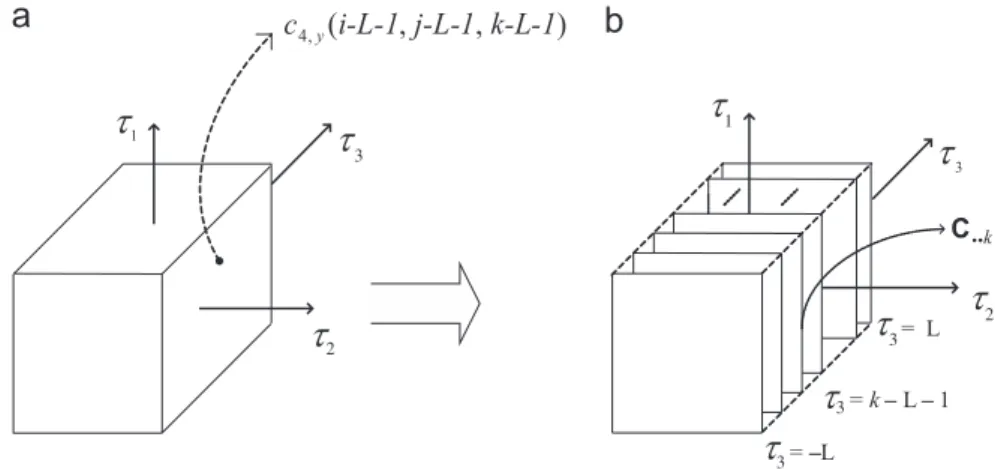
where the element in positionði;j;kÞcorresponds to

cijk¼c4;yðiL1;jL1;kL1Þ as shown

inFig. 1a. Replacing (11) into (13), we can write the tensorCð3;yÞ _{as a sum ofLþ1 outer products, each}

one involving 3 vectors, as follows:

Cð3;yÞ_¼g 4;s

XL

l¼0

h_lHlþ1Hlþ1Hlþ1, (14)

where Hlþ1¼P2_pL_¼1þ1hlþpL1eð2pLþ1Þ. Eq. (14)

re-presents the Parafac decomposition of the tensor

Cð3;yÞ_{. Let us define the channel coefficient matrix}

H2Cð2Lþ1ÞðLþ1Þ as follows:

H9H_{ðhÞ ¼ ½H1H2}. . ._HLþ1

¼

0 0 h0

. . . _.

. . _.

.

. _.

. .

0 h0 hL1

h0 h1 hL

. . . _.

. . _.

.

. _.

. .

hL1 hL 0

hL 0 0

0

B B B B B B B B B B B B B B B B @

1

C C C C C C C C C C C C C C C C A

, (15)

where H_{ðÞ is an operator that builds a Hankel}

matrix from its vector argument as shown above and the channel coefficient vector is defined as

h¼ ½h0. . .hLT2CðLþ1Þ. (16)

In the next section, we establish a link between the Parafac decomposition (14) and the simulta-neous matrix diagonalization approach. Then, we present a SS LS algorithm to blindly estimate the channel coefficient vector.

4. Blind SISO channel identification using the Parafac decomposition of the 4th-order output cumulant tensor

Slicing the cumulant tensorCð3;yÞ_{along each of its}

three dimensions yields 2Lþ1 cumulant matrices

Ci, Cj and Ck, i;j;k2 ½1;2Lþ1, respectively,

each of which being of dimensions ð2Lþ1Þ ð2Lþ1Þ. In Fig. 1b we show the frontal slices

Ck, obtained by fixing the third indexk, which are

given by

Ck¼

X

2Lþ1

i¼1

X

2Lþ1

j¼1

cijkeð2i Lþ1Þe

ð2Lþ1ÞT

j

¼g4;s

XL

l¼0

h_lhlþkL1HlHHl

¼g_4;sHDkðRÞHH, (17)

fork2 ½1;2Lþ1, where

R¼HDiagð Þh 2Cð2Lþ1ÞðLþ1Þ. (18) Notice that the frontal slices defined in (17) have the form ofTkinTable 2with the three loading factors

depending on Has follows:

Að1Þ¼H; Að2Þ¼H and Að3Þ ¼g4;sR. (19)

Hence, by analogy with the other equations in

Table 2, we get the following expressions of the vertical and horizontal slices:

Cj¼g4;sRDjðHÞHT; j2 ½1;2Lþ1, (20)

Ci¼g4;sHDiðHÞRT; i2 ½1;2Lþ1. (21)

It is interesting to note that Eqs. (17), (20) and (21) suggest that the Parafac components of the cumulant tensor can be obtained from the factor-ization of a 2D slice or, more precisely, from the simultaneous diagonalization of a set of matrices, such as Ck, k2 ½1;2Lþ1. However, since the

channel matrix H is not unitary, it cannot be recovered from a simple application of a diagona-lization technique, such as SVD,3 without a previous orthonormalization of the slicesCk. This

extra operation, often referred to as pre-whitening, consists in constructing a new set of modified

cumulant matrices that admit an orthogonal decomposition. The modified cumulant matrices are obtained by means of a linear transformationW

so that C¯k¼WCkWH, with WH unitary. The

computation of matrixWusually requires resorting to SOS. This additional step, very common in HOS-based methods [10,44,45], is time-consuming and often responsible for increased estimation errors

[30,31]. Without resorting to a tensor formalism, the joint-diagonalization approach is exploited in

[11], using cumulant matrices that can be obtained from (17), with non-negative time-lags only, i.e. 0pt1;t2;t3pLor, equivalently:

Lþ1pi;j;kp2Lþ1.

Eq. (14) shows that the rank of tensor Cð3;yÞ

equals the numberFof non-zero coefficients inh, so thatFpLþ1. Assumption A4 ensures that FX2. Due to its Hankel structure, His full column-rank and thenk_Að1Þ ¼k_Að2Þ ¼rH¼Lþ1. From (18) and

assumption A4, we deduce thatrS¼FX2. If all the

channel coefficients are nonzero, then F ¼Lþ1 and we havek_Að3Þ ¼rR¼Lþ1; otherwisekAð3Þ ¼0

because, if FoLþ1, at least one column of

R is zero. From the Kruskal uniqueness condi-tion (4), we conclude that, if F¼Lþ1, then

k_Að1Þþk_Að2Þþk_Að3Þ ¼3Lþ3X2Fþ2; otherwise,

if FoLþ1, then k

Að1ÞþkAð2ÞþkAð3Þ ¼2Lþ2X

2Fþ2, which implies that the Kruskal condition is always satisfied. Thus, any set fA¯ð1Þ;A¯ð2Þ;A¯ð3Þg

satisfying the Parafac decomposition of the cumu-lant tensorCð3;yÞ_{has the form (3), withA}ð1Þ_,Að2Þ_and

Að3Þ given in (19).

Tensor Cð3;yÞ _{can be expressed under unfolded}

matrix representations obtained by stacking up the 2D slices (17), (20) or (21). Taking the equations in

Table 2into account and using the correspondences (19), we obtain the equations in Table 3. These unfolded matrices can be used to estimateHand_R by means of the TALS algorithm. Once H is estimated it is straightforward to deduce the channel parameters. However, we can improve the efficiency of the estimation procedure by coupling both estimation steps, i.e. taking the relationships be-tween the channel coefficient vector h and the matrices H and R into account, thus eliminating column scaling and permutation ambiguities[46,47].

SS-LS Parafac-based blind channel identification algorithm

In this section, we propose a SS-LS algorithm to estimate the channel coefficient vectorhby means of the previously described tensor decomposition. Using (18), we can express C½1 (given in Table 3)

as follows:

C½1¼g4;sðH HÞDiagð Þh HT. (22)

Applying property (P-1) to this equation, we get vecðC½1Þ ¼g4;sðH H HÞh. (23)

The channel coefficient vectorh can be obtained by iteratively minimizing the following LS cost function:

cðh;h^ðr1ÞÞ9kvecðC½1Þ g4;sG^ðr1Þhk2, (24)

where

^

Gðr1Þ ¼H^ðr1Þ H^ðr1Þ H^ðr1Þ (25) and, from (15),H^ðr1Þ¼H_ðh^ðr1Þ_{Þ. At iterationr, we}

get h^ðrÞ ¼arg mincðh;h^ðr1ÞÞ. The algorithm is

initialized with a Hankel matrix H^ð0Þ in which the first column is ½0T_ðLÞ h^ð0ÞTT and the last row is

½h^ð0Þ_L 0T_ðLÞ, where h^ð0Þ ¼ ½1 vTT_{, v2C}ðLÞ _{is a}

Gaus-sian random vector and0ðLÞis an all-zeros vector of

dimension L. The algorithm is iterated until

kh^ðrÞh^ðr1Þk=kh^ðrÞkpe, where e is an arbitrary

small positive constant. In order to take the constraint h0¼1 into account at each iteration r,

we normalize the previous estimate h^ðr1Þ with respect to its first entry h^ð₀r1Þ before using it to update H^ðr1Þ using (15). Then, G^ðr1Þ is updated from (25) using H^ðr1Þ. The normalization step eliminates the scaling ambiguity and forcing the Hankel structure allows us to avoid column permutation in the Parafac decomposition.

The above described strategy ensures the Hankel structure ofHat each iteration, taking advantage of its full-rank property to make the tensor decom-position essentially unique and the channel estima-tion free from ambiguities. Furthermore, a SS-LS minimization procedure is used instead of the classical trilinear ALS algorithm. For that reason, our method should be expected to increase the convergence speed. After initializing h^ð0Þ as a Gaussian random vector, the SS-LS Parafac-based Blind Channel Identification (SS-LS PBCI) algo-rithm can be summarized as follows, for rX1:

1. Use (15) to build H^ðr1Þ¼H_ð1=h^ðr1Þ 0 h^

ðr1Þ

Þ. 2. ComputeG^ðr1Þ using (25).

3. Minimize the cost function (24) so that

^

hðrÞ¼g1_4;sG^ðr1Þ#vecðC½1Þ. (26)

4. Iterate until kh^ðrÞh^ðr1Þk=kh^ðrÞkpe.

The identifiability of the channel coefficient vector h depends on the rank of the matrix

^

Gðr1Þ2Cð2Lþ1Þ3ðLþ1Þ_{. Due to its Hankel structure,}

given by (15), H^ðr1Þ is ensured to be full column-rank. So, we have k_H^ðr1Þ ¼Lþ1 and therefore

^

Gðr1Þ, defined in (25) as a double Khatri–Rao product, is also full column-rank[48], which implies the uniqueness of the LS solution given by (26).

5. MIMO channel model and 4th-order spatial cumulant tensors

Let us consider an instantaneous MIMO channel withQsignal sources andMreceive antennas. The

Table 3

Parafac formulae for the 3rd-order tensorCð3;yÞ

Direction Tensor 2D slices Unfolded representations Horizontal Ci¼g4;sHDiðHÞRT C½1¼g4;sðH HÞRT

Vertical Cj¼g4;sRDjðHÞHT C½2¼g4;sðH RÞHT

signals received at the front-end of the antenna array at the time-instant n, are modeled as a complex-valued vectoryðnÞ 2CM _{written as}

yðnÞ ¼HsðnÞ þtðnÞ, (27)

where the elements of the instantaneous mixing matrix H2CMQ _{are the MIMO channel}

coeffi-cientshmq. The following assumptions are made:

B1. The source signalssqðnÞare stationary, ergodic

and mutually independent with symmetric distribution, zero-mean and non-zero kurtosis

g₄;sq ¼c4;sqð0;0;0Þassumed to be known.

B2. The vectortðnÞ 2CM1is the additive Gaussian

noise at the output of the antenna array. It is independent from the source signals and has an unknown spatial correlation.

B3. The MIMO channel matrix H2CMQ has elements hm;q, representing a Rayleigh flat

fading propagation environment, i.e. the chan-nel coefficients are complex constants with real and imaginary parts driven from a continuous Gaussian distribution.

Assuming that g_4;sq is known is not really constraining in the context of telecommunication systems, where the source modulation schemes are generally known at the receiver. Although usual, this assumption is not absolutely necessary and could be relaxed. Note also that we do not constrain the source kurtoses to have equal sign. Assumption B3 allows us to say that H is full k-rank with probability one, even whenMoQ.

We now consider the blind MIMO channel identification problem using 4th-order output sta-tistics only. It is well known that solutions to this problem only exist up to a column scaling and permutation indeterminacy. The 4th-order spatial cumulants of the array outputs are defined as

C4;yði;j;k;lÞ9cum½yiðnÞ;yjðnÞ;ykðnÞ;ylðnÞ. (28)

Under the above mentioned assumptions, it is straightforward to show that

C4;yði;j;k;lÞ ¼

X

Q

q¼1 g₄;sqh

iqhjqhkqhlq, (29)

Notice that the cumulants C4;yði;j;k;lÞ only exist

for 1pi;j;k;lpM. Let us define the 4th-order tensor Cð4;yÞ₂CMMMM_{, in which the element}

in position ði;j;k;lÞ corresponds to C4;yði;j;k;lÞ,

so that

Cð4;yÞ _¼ X

M

i¼1

XM

j¼1

XM

k¼1

XM

l¼1

C4;yði;j;k;lÞeðiMÞ

eð_jMÞe_kðMÞeð_lMÞ. (30) Replacing (29) into (30) we can rewrite Cð4;yÞ _{as a}

sum ofQrank-1 tensors, each one being written as an outer product involving four vectors:

Cð4;yÞ _¼X

Q

q¼1

H_qHqHq ðg4;sqHqÞ, (31)

whereHq¼PMm¼1hm;qeðmMÞ,q2 ½1;Q. Eq. (31) is the

Parafac decomposition of tensor Cð4;yÞ_{, where the}

four loading factors depend onH, as follows:

Að1Þ ¼H; Að2Þ¼H; Að3Þ¼H

and

Að4Þ ¼HC4;s, (32)

where

C4;s¼Diagðg4;s₁;. . .;g4;s_QÞ. (33)

Using the above correspondences, the 2D repre-sentations of Cð4;yÞ _{can be deduced from the}

equations in Table 1. For instance, slicing Cð4;yÞ

along the kl plane gives the following matrix

C½1;22CM

3_M

:

C½1;2¼ ðH H HÞC4;sHT. (34)

According to the unfolding procedure described in Section 2, C½1;2 is obtained4 by stacking matrices

C½2i, i2 ½1;M, defined as C½2i¼ ½C

T

i1;. . .;CTiMT,

where Cij are the 2D slices of tensor Cð4;yÞ along

the kl plane, with ½Cijkl ¼C4;yði;j;k;lÞ,

k;l2 ½1;M.

From the general equations given inTable 1, we easily get Cij¼HDiðHÞC4;sDjðHÞHT. This

for-mulation naturally leads to a simultaneous diag-onalization problem. A similar set of equations can be obtained from the output quadricovariance matrix, which is the basic idea behind the FOBIUM algorithm[49]. In fact, FOBIUM can be viewed as a 4th-order extension of the classic SOS-based SOBI algorithm [10]. Indeed, it needs a 4th-order pre-whitening step and requires non-Gaussian sources having kurtoses with the same sign and different

4_{In practice, thelth-column ofC}

½1;2is formed with the elements C4;yði;j;k;lÞarranged in such a way that the indicesi;j;k2 ½1;M

trispectra. By exploiting the Kronecker structure of a particular unfolded tensor representation, the method reported in[32]solves the canonical tensor decomposition problem by means of a simultaneous matrix diagonalization. Making use of similar ideas, the algorithms proposed in [14] have the advantage of permitting weaker uniqueness condi-tions and hence, theoretically allowing for the identification of more sources for a fixed number of antennas. Although avoiding pre-whitening, these latter algorithms still have to solve two optimization problems in order to extract MIMO parameters from an initial EVD-based estimate. On the contrary, we propose solutions that can be obtained from a single minimization problem, under very mild assumptions.

5.1. Uniqueness

Notice from (31) that the rank of the 4th-order tensor Cð4;yÞ _{is F¼Q. In addition, since H is}

assumed to be full k-rank, we have k_Að1Þ ¼k_Að2Þ ¼

k_Að3Þ¼k_Að4Þ ¼rH¼minðM;QÞ. We conclude from

(4) that the Kruskal uniqueness condition reduces to

4rHX2Qþ3. (35)

The two following cases can be considered:

The MIMO channel is an overdetermined sys-tem, i.e. MXQ. In this case rH¼Q and (35)

states that the Parafac decomposition ofCð4;yÞ _is

essentially unique ifQX3=2, i.e.Q41. There are

no further constraints on the number of sensors.

The MIMO channel is an underdetermined system, i.e. MoQ. In this case r_H ¼M and

hence equation (35) becomes

Qp2M2. (36)

Table 4gives the maximum number of users that our model can deal with, for a given number of receiving antennas varying fromM¼2 to 7. Under these conditions, the Parafac decomposition of tensor Cð4;yÞ _{is unique, up to trivial permutation}

and scaling ambiguities. In other words, the loading

factors ofCð4;yÞ _{are given by (3) withA}ð1Þ_,Að2Þ_,Að3Þ

andAð4Þ defined in (32).

5.2. Reduced-order cumulant tensor

It is possible to reduce the 4th-order tensor defined in (30) to a 3rd-order one by combining its 3D slices, thus reducing the complexity of the above described tensor decomposition. Without loss of generality, we freeze the index k in the cumulant definition (28), and define the 3D slices as

Cð3;yÞ

k ¼

XM

i¼1

XM

j¼1

XM

l¼1

C4;yði;j;k;lÞeðiMÞe

ðMÞ

j e

ðMÞ

l

(37)

¼ X

Q

q¼1

g_4;sqh_kqH_qHqHq. (38)

Summing these slices for all k2 ½1;Mwe get

Cð3;yÞ_¼X

M

k¼1 Cð3;yÞ

k ¼

X

Q

q¼1

H_qHq g4;sqHq

XM

k¼1

h_kq !

.

(39)

From this equation, we conclude that Cð3;yÞ _{is a}

3rd-order Parafac model with the following loading factors:

Að1Þ¼H;Að2Þ ¼H and Að3Þ ¼HDC4;s, (40)

whereDis a diagonal matrix given by

D¼X

M

k¼1

DkðHÞ. (41)

Using the correspondences (40) in the equations of Table 2, we get the unfolded representations of tensor Cð3;yÞ_{. Selecting, for instance, the horizontal}

slicing direction (first row inTable 2), we have

C½1¼ ðH HÞC4;sDHT. (42)

In practice,C½1is obtained by stacking the matrices

Ci, i2 ½1;M, where ½Cijl¼

P

kC4;yði;j;k;lÞ,

j;l2 ½1;M. This is equivalent to ½C½1ði1ÞMþj;l¼

P

kC4;yði;j;k;lÞ,i;j;l2 ½1;M.

Due to assumption B3, the diagonal entries of_D are nonzero with probability one. This allows us to conclude thatk_Að1Þ¼k_Að2Þ¼k_Að3Þ ¼rH¼minðM;QÞ

and the Kruskal uniqueness condition (4) becomes 3rHX2Qþ2. This yields QX2 for MXQ and

Qpð3M2Þ=2 when MoQ. Table 5 shows the maximum number of sources for a given number of receive antennas varying from M¼2 to 7 so that

Table 4

the model is unique. Under these conditions, the Parafac loading factors ofCð3;yÞ _{can be written as in}

(3) with Að1Þ,Að2Þ andAð3Þ defined in (40).

6. Parafac-based blind MIMO channel identification (PBMCI) algorithms

Based on the explicit relationships presented in the previous section, we now propose two algo-rithms to estimate the instantaneous MIMO mixing matrix, up to column scaling and permutation. This is achieved by means of a single (non-alternating) LS minimization procedure, thanks to the symmetry properties of the 4th-order cumulant. The basic idea behind the algorithms proposed in the sequel is to consider only one of the unfolded representations of the cumulant tensorCð4;yÞ_{by exploiting the}

relation-ships (32) (or (40) in the case of Cð3;yÞ_{). This is}

equivalent to rewrite any of the unfolded tensor representations defined inTable 1(resp.Table 2) in terms of AðpÞ, for a fixed p. After that, we also present the procedures for estimating the mixing matrix using the classical ALS-type algorithms described in Section 2.

6.1. 4D SS-LS PBMCI algorithm

Eq. (34) enables us to estimate the MIMO channel matrix by iteratively minimizing a single LS cost function, written as follows:

cðH^r1;HÞ9kC½1;2 ðH^r1 H^r1 H^r1ÞC4;sHTk2F,

(43)

whererdenotes the iteration number. The iterative minimization ofcðH^r1;HÞyields the following LS

solution:

^

HT_r9arg min

H cð

^

Hr1;HÞ

¼_C1_4;sðH^_r1 H^r1 H^r1Þ #

C½1;2, (44)

where H^0 is initialized as a complex MQ

Gaussian random matrix. In order to improve estimation at each iterationrX1, before computing

^

Hr, we normalize each column of the previous

estimate H^r1 by dividing it by its 2-norm. The

algorithm is stopped whenkH^rH^r1kF=kH^rkFpe,

whereeis an arbitrary small positive constant. In the underdetermined case, the uniqueness of the Parafac decomposition ofCð4;yÞ_{is ensured under}

the condition stated by the Kruskal Theorem (4), which leads to the relationships between Mand Q

given in Table 4. Due to the lemma introduced in

[48], ifkHþkHXQþ1 thenH His full

column-rank, which yields kH _H ¼Q. In the

underdeter-mined case, we have kH¼M and hence the

previous condition becomes Qp2M1. Applying the same lemma on the double Khatri–Rao product

H H H, the condition kH _Hþk_HXQþ1 is

equivalent to QþMXQþ1, which is always

satisfied, implying that the double Khatri–Rao product is full column rank, which guarantees the uniqueness of the LS solution given by (44). Notice that this constraint is slightly weaker than the uniqueness condition (36), so that, by satisfying this latter one, we can ensure that any matrixH¯ obeying to (34) is such that H¯ ¼HKP, where P is a permutation matrix and Ka diagonal matrix with unit-modulus diagonal elements. Therefore, since we are dealing with complex values, the scaling ambiguity is not completely eliminated but it is reduced to a single phase indeterminacy. The above described method will be referred to as the 4D SS-LS Parafac-based Blind MIMO Channel Identification (4D SS-LS PBMCI) algorithm. The above developments were presented, without loss of generality, forC½1;2. Any other equation inTable 1

can be used instead.

6.2. 3D SS-LS PBMCI algorithm

The SS approach can also be formulated using tensor Cð3;yÞ _{defined in (39). Eq. (42) yields the}

following LS cost function:

cðH^r1;HÞ9kC½1 ðH^r1 H^r1ÞC4;sD^r1HTk2F,

(45)

where D^r1¼PkDkðH^r1Þ. Iteratively minimizing

(45) leads to

^

HT_r ¼C14;sD^

1

r1ðH^r1 H^r1Þ #

C½1. (46)

Here again, H^0 is initialized as a complex MQ

Gaussian random matrix and H^r1 is normalized

before computing the next estimateH^r. This method

will be called the 3D SS-LS PBMCI algo-rithm. Sufficient uniqueness conditions are given

Table 5

Relationship betweenMandQfor the uniqueness of the Parafac decomposition ofCð3;yÞ

in Table 5. According to the lemma introduced in

[38], we needQp2M1 in order to ensure that the

Khatri–Rao product in (46) is full column-rank, which guarantees the uniqueness of the LS solution. This condition is weaker than the uniqueness conditions discussed in Section 5.2.

6.3. ALS-type PBMCI algorithms

Classical ALS-type algorithms can also be used to solve the blind channel identification problem. In particular, the QALS and TALS algorithms de-scribed in Section 2 provide solutions to the Parafac decomposition of tensorsCð4;yÞ _andCð3;yÞ_{, using the}

equations provided inTables 1 and 2, respectively. Although these algorithms do not take the relation-ships between the loading factors into account, we can nevertheless initialize QALS with a complex

MQ Gaussian random matrix A^ð2Þ₀ and then deduce A^ð3Þ₀ and A^ð4Þ₀ using (32). After that, the QALS algorithm is started with the computation of

^

Að1Þ₁ using (7).

Denoting by r¼ 1 the iteration at which convergence is reached, the estimated loading factorsA^ð₁pÞ,p¼1;. . ._{;4, have the form (3). Taking}

the correspondences (32) into account, this yields the following different equations for estimatingH, up to column scaling and permutation:

^

Að1Þ₁ ¼H^ð1ÞK1P,

^

Að2Þ₁ ¼H^ð2ÞK2P,

^

Að3Þ₁ ¼H^ð3ÞK3P,

^

Að4Þ₁ ¼H^ð4ÞC4;sK4P. (47)

The estimates H^ð1Þ and H^ð3Þ can be obtained by simple conjugation of A^ð1Þ₁ and A^ð3Þ₁, respectively. The above procedure will be referred to as the quadrilinear ALS Parafac-based blind MIMO channel identification (QALS-PBMCI) algorithm.

Concerning the TALS algorithm, it can also be initialized with a complexMQGaussian random matrixA^ð2Þ₀ andA^ð3Þ₀ is deduced from (40) and (41). The correspondences (40) indicate that the loading factors A^ð1Þ₁, A^ð2Þ₁ and A^ð3Þ₁ are estimates of H, up to column permutation and scaling. This method will be called the trilinear ALS Parafac-based blind MIMO channel identification (TALS-PBMCI) algorithm.

Although scaling and permutation ambiguities are not explicitly solved, these indeterminacies do

not represent a concern in the context of blind mixture identification and, in the overdetermined case, it is even possible to recover the source signals.

7. Computer simulations

In this section, we present some computer simulation results in order to assess the performance of the proposed blind identification algorithms. We first consider a SISO-FIR communication channel and compare the performance of the SS-LS PBCI method with the results obtained using the well-known FOSI algorithm, which is based on a joint diagonalization technique. As suggested by the authors of [11], the FOSI algorithm performance is evaluated by averaging the results of the two solutions proposed therein. We also compare our method with the optimal algebraic solution in the total least squares (TLS) sense, proposed in [5].

Afterwards, we consider a quasi-static MIMO channel scenario where the complex channel coeffi-cients are drawn from a Rayleigh distribution and are assumed to be time-invariant within the dura-tion of a time-slot, composed of Nsymbol periods. The performance of the QALS-PBMCI and TALS-PBMCI algorithms are compared with those of the SS-LS PBMCI algorithms. Although our main interest is in mixture identification, we also provide results concerning the recovery of the transmitted symbols using the channel estimates obtained with the proposed identification methods in both SISO and MIMO cases.

7.1. SISO channel identification

The parametric channel estimation performance is evaluated by means of the normalized mean squared error (NMSE) of the estimator, computed by means of the following formula:

NMSE_¼1

P

XP

p¼1

kh^ð1Þ_hpi hk2

khk2 , (48)

nonminimum-phase as well as maximum-phase channels may occur. Furthermore, we allow for some channels to be possibly ill-conditioned (hL

very small in magnitude). The results illustrated in the following curves represent the average of P¼

200 Monte Carlo runs. The input signal is QPSK modulated.

InFig. 2, the NMSE is plotted against the signal-to-noise ratio (SNR) for SS-LS PBCI, FOSI and TLS algorithms. The curves on the left-hand side show that our approach performs better than both, the FOSI algorithm and the TLS solution, for channels with memory L¼3. The relative behavior of the algorithms shown in that figure was also verified for L¼2 and 4. On the right-hand side ofFig. 2, we compare the results of SS-LS PBCI for L¼4 with those of the FOSI algorithm for L¼2;3 and 4. Note that the estimation errors obtained with SS-LS PBCI for

L¼4 are smaller than those of FOSI forL¼4 and 3. Furthermore, for low SNR values, the perfor-mance provided by the SS-LS PBCI algorithm for channels with L¼4 is close to that obtained with FOSI for channels with L¼2. We can therefore conclude that, increasing the channel delay spread, the SS-LS PBCI method provides better perfor-mance than the two other algorithms, especially in highly noisy situations.

In order to evaluate the effect of the output data sequence length used to estimate the 4th-order cumulants over the performance of the identi-fication algorithms, we plot in Fig. 3 the NMSE against the channel memory for N¼1000 and 3000 output data, with SNR¼21 dB. We can conclude that SS-LS PBCI with N¼1000 yields better results than TLS and FOSI algorithms with

N¼3000.

0 5 10 15 20 25

−20 −15 −10 −5

0 5

SNR (dB)

NMSE (dB)

L = 3

FOSI TLS

0 5 10 15 20 25

−20 −15 −10 −5

0 5

SNR (dB)

NMSE (dB)

FOSI, L=4 FOSI, L=3 FOSI, L=2

SS−LS PBCI SS−LS PBCI, L=4

Fig. 2. NMSE performance with QPSK modulation.

1 2 3 4

−35 −30 −25 −20 −15 −10 −5

0

Channel memory (L)

NMSE (dB)

TLS FOSI

N=1000 samples N=3000 samples SS−LS PBCI

Fig. 3. NMSEchannel memory with SNR¼21 dB.

1 2 3 4

0 50 100 150

MEAN

initialization: random initialization: TLS initialization: C(q,k)

1 2 3 4

0 50 100

Channel memory (L)

MEDIAN

initialization: random initialization: TLS initialization: C(q,k)

Number of iterations for convergence of SS−LS PBCI

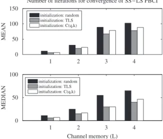
It is interesting to note that the number of iterations required for convergence of the SS-LS PBCI algorithm can be reduced by initializing it with an algebraic solution such as the TLS solution. InFig. 4we show the mean and median number of iterations needed for convergence of SS-LS PBCI with SNR¼21 dB using three different initializa-tions: (1) a Gaussian random vector; (2) the TLS solution and (3) the Cðq;kÞ solution [50]. Using either the TLS or theCðq;kÞsolutions as initializa-tion decreases the number of iterainitializa-tions in compar-ison with the random initialization. Finally, it is worth to mention that the NMSE performance after convergence remains unchanged, i.e. initialization only affects convergence speed.

7.1.1. Recovery of the input signal

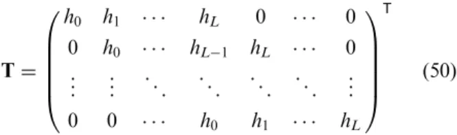
Several equalization approaches exist to recover the input data sequence using the estimated channel. The optimal solution in the minimum mean squared error (MMSE) sense is provided by the Wiener solution. The coefficient vectorw2CðKþ1Þ1 of the optimal equalizer is given by

wðoptÞ ¼ ðTHTþs2_uIðLþ1ÞÞ1THsd, (49)

whereTis aðKþLþ1Þ ðLþ1ÞToeplitz matrix built from the channel coefficients as follows:

T¼

h0 h1 hL 0 0

0 h0 hL1 hL 0

. . . _.

. . _.

.

. _.

.

. _.

. . _.

. . _.

. .

0 0 h0 h1 hL

0

B B B B @

1

C C C C A

T

(50)

andsd ¼eðdKþLþ1Þ, where d represents the

equaliza-tion delay, usually chosen as d¼ ðKþLþ1Þ=2 if

KþLis odd ord ¼ ðKþLþ2Þ=2 ifKþLis even.

The input signal is recovered as follows:

^

sðnÞ ¼X

K

k¼0

wðoptÞ_k yðnkÞ. (51)

In Fig. 5, we present the performance of SS-LS PBCI and FOSI algorithms in terms of the symbol error rate (SER) for channels with L¼2 (left) and L¼3 (right), and a QPSK modulated input signal. The dotted lines represent the results obtained with the optimal MMSE filter assuming perfect knowledge of the channel. For a target SER of 103, withL¼2, SS-LS PBCI provides a gain of about 5 dB in SNR with respect to FOSI. For

L¼3, despite the expected performance loss of both algorithms, this gain is around 8 dB in SNR for a target SER of 2103.

7.2. MIMO channel identification

In this section, we consider a quasi-static trans-mission scenario where the complex MIMO channel coefficients are drawn from a Rayleigh distribution and are assumed to be time-invariant within the duration of a time-slot composed of N symbol periods. At each new time-slot the channel varies independently. Except otherwise stated, the length of the time-slot isN¼1000 symbol periods and the output data samples received in this interval are used to estimate the spatial cumulants. Our results are averaged over 300 time-slots.

In order to evaluate the performance of the proposed Parafac-based blind MIMO channel identification algorithms, we utilize the identi-fication performance index given in [51,52], which is based on the matrix Uhpi¼H#H^hpi, where H^hpi

is the channel estimate after convergence of the

0 5 10 15 20 25 10−5

10−4 10−3 10−2

SNR (dB)

SER

L = 2

0 5 10 15 20 25 SNR (dB)

SER

L = 3

FOSI Opt. MMSE

10−5 10−4 10−3 10−2 SS−LS PBCI

FOSI Opt. MMSE SS−LS PBCI

experimentp2 ½1;P. Since we estimate the channel up to column scaling and permutation, it is easy to conclude that Uhpi is a scaled permutation matrix. The identification performance index is computed as follows:

xð_UhpiÞ91 2

X

i

X

j

jfh_i;p_jij2

max‘jfh_i;‘pij2 !

1

! "

þ X

j

X

i

jfh_ip_;jij2

max‘jfh‘;pjij

2

!

1

!#

, (52)

wherefh_i;p_ji are the entries ofUhpi. The performance indexxðÞequals zero if its matrix argument has the exact structure of a scaled permutation matrix, and small values indicate proximity to the desired solution. In our case, xð_Uhpi_{Þ tends towards zero}

when the channel estimate approximates the actual MIMO channel matrix, up to column scaling and permutation. Eq. (52) provides, therefore, a mea-sure of the global level of interference rejection

between the estimated channels, irrespective of the trivial ambiguities. In the following figures, we plot the value of the average performance index, i.e.

ð1=PÞPP

p¼1xðU

hpi_{Þ, whereP¼300 is the number of}

time-slots (Monte Carlo simulations).

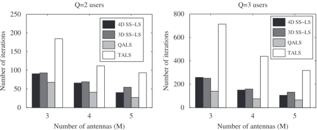
We first evaluate the PBMCI approach by comparing the proposed algorithms 4D SS-LS and 3D SS-LS with their ALS-based counterparts (QALS and TALS, respectively). Using M¼3 sensors, we show inFig. 6the average identification performance index computed using (52) in function of the SNR forQ¼2 (left) andQ¼3 (right) QPSK modulated sources. We can conclude that the methods based on 4th-order tensors (4D SS-LS and QALS) performed better than their 3rd-order versions (3D SS-LS and TALS). As expected, increasing the number of sources degrades the performance, but 4D SS-LS is less affected than the other methods.

InFig. 7, we show the mean number of iterations needed for convergence of the four algorithms when

0 5 10 15 20 25

10−4 10−3 10−2 10−1 100

101

SNR (dB)

Performance inde

x

Q = 2, M = 3

0 5 10 15 20 25

SNR (dB)

Performance inde

x

Q = 3, M = 3

QALS TALS

QALS TALS

10−4 10−3 10−2 10−1 100

101

Fig. 6. Average identification performance indexSNR.

3 4 5

0 50 100 150 200 250

Number of iterations

Number of antennas (M) Q=2 users

4D SS−LS

3D SS−LS

QALS

TALS

3 4 5

0 200 400 600 800

Q=3 users

Number of iterations

Number of antennas (M) 4D SS−LS

3D SS−LS

QALS

TALS

Q¼2 (left) and Q¼3 sources (right) with SNR¼

21 dB. Although 4D SS-LS takes generally more iterations to converge than QALS, the former one is a more attractive solution due to its smaller computational complexity, since it involves only one LS minimization per iteration, instead of four. Note that increasing the number of users for a given number of antennas significantly increases the number of iterations needed for convergence. As expected, the methods based on the 4th-order tensor converge faster than those based on the 3rd-order one. Finally, we observe that the algorithms take more iterations to converge when the number of antennas decreases, i.e. when the spatial diversity decreases.

As recent papers have compared new approaches with several classical blind channel identification algorithms (cf. see [13]) we compare our methods with some of the most performing algorithms reported in the literature. In the sequel, we show some simulation results comparing the identification performance of the 4D SS-LS PBMCI with the classical JADE [9]algorithm, the FOOBI [14] and

the ICAR [13] methods. The SOBI algorithm [10]

and its counterpart to high-order cumulants (FOBIUM [49]) have not been considered because they are theoretically unable to deal with sources that have similar trispectra.

ForQ¼2 users andM¼3 antennas,Fig. 8(left) shows that the 4D SS-LS PBMCI performance is close to that of the ICAR and FOOBI algorithms. Note that JADE degrades when the noise power increases, becoming less performing than the other methods for SNR lower than 12 dB. For Q¼3 sources andM¼3 antennas,Fig. 8(right) indicates that our approach performs better than the other tested algorithms. We have also simulated the case of M¼5 antennas and observed improved results for all the algorithms. For instance, withM¼5 and

Q¼3, JADE becomes better than 4D SS-LS for SNRX7:5 dB. Besides, ICAR and FOOBI also take

advantage of the additional degrees of freedom and both attain nearly the same performance as 4D SS-LS. In these scenarii, 4D SS-LS seems to be a very interesting solution, especially when noise becomes important and the ratioM=Qis close to one.

0 5 10 15 20 25

10−4 10−3 10−2 10−1 100

101

SNR (dB)

Performance inde

x

Q = 2, M = 3

FOOBI ICAR JADE

0 5 10 15 20 25

SNR (dB)

Performance inde

x

Q = 3, M = 3

FOOBI ICAR JADE

10−4 10−3 10−2 10−1 100

101

Fig. 8. Comparison with other algorithms.

0 5 10 15 20 25

10−5 10−4 10−3 10−2 10−1 100

SNR (dB)

SER

Q = 2

Opt. MMSE, M=3 Opt. MMSE, M=5

0 5 10 15 20 25

SNR (dB)

SER

Q = 3

Opt. MMSE, M=3

Opt. MMSE, M=5

10−5 10−4 10−3 10−2 10−1 100