TENSOR-BASED BLIND IDENTIFICATION OF MIMO VOLTERRA CHANNELS IN
A MULTIUSER CDMA ENVIRONMENT
Carlos Alexandre R. FERNANDES , G´erard FAVIER, and Jo˜ao C. M. MOTA
I3S Laboratory
University of Nice-Sophia Antipolis/CNRS 2000 route des Lucioles, BP 121,06903
Sophia-Antipolis Cedex, France.
phone: + (33) 492942736, fax: + (33) 492942896 email:{acarlos,favier}@i3s.unice.fr
Dep. de Engenharia de Teleinform´atica Universidade Federal do Cear´a
Campus do Pici, 60.755-640,6007 Fortaleza, Brazil. phone: +(55 85) 33669467 Fax:+(55 85) 33669468 email: [email protected], [email protected]
ABSTRACT
This paper is concerned with the blind identification of Multiple-Input-Multiple-Output (MIMO) Volterra channels in a multiuser Code Division Multiple Access (CDMA) environment. The channel is modeled using the most generic representation of complex-valued Volterra systems. A Parallel Factor (PARAFAC) decomposition of a third-order tensor composed of channel output covariances is used, the transmitted signals being assumed to be Phase Shift Keying (PSK) modulated. The channel estimation is carried out by two algorithms: the Alternating Least Squares (ALS) algorithm and a non-iterative least squares algorithm that exploits the redundancy provided by the Khatri-Rao product. The perfor-mance of the proposed estimation methods is illustrated by means of computer simulations.
1. INTRODUCTION
This paper proposes two blind identification methods for identify-ing Multiple-Input-Multiple-Output (MIMO) Volterra channels in the context of a multiuser Code Division Multiple Access (CDMA) communication system. The channel is modeled as the most generic representation of complex-valued Volterra systems. This kind of nonlinear models has important applications in the field of telecom-munications, e.g. to model uplink channels in Radio Over Fiber (ROF) multiuser communication systems [1, 2, 3], the nonlinearity of which is introduced by the electrical-optical conversion. These links can be modeled as a MIMO Wiener filter, that constitutes a particular case of MIMO Volterra filters. Another application of such models can be found in CDMA systems with power ampli-fiers driven at or near saturation to achieve the power consumption requirements [4].
The proposed identification methods use second-order statis-tics of the signals received by an antenna array, assuming that the transmitted signals are Phase Shift Keying (PSK) modulated. These methods are based on a Parallel Factor (PARAFAC) decomposition [5] of a third-order tensor (three way array) composed of channel output covariances. One of the great advantages of these methods is that they allow working with weak uniqueness conditions compared with previous works [4, 6, 7, 8], that require a number of channel outputs greater than the number of Volterra filter parameters. In-deed, the proposed tensor-based algorithms provide a great flexibil-ity on the number of antennas, which is particularly important when identifying Volterra systems. Moreover, PARAFAC decomposition avoids the use of a pre-whitening step, an operation that increases the computational complexity and may degrade the channel estima-tion.
The PARAFAC decomposition is first carried out by a two-steps Alternating Least Squares (ALS) algorithm [5]. As the ALS algo-rithm may need many iterations to converge [9], a non-iterative es-timation method exploiting the redundancy of the Khatri-Rao
prod-C. A. R. FERNANDES is scholarship supported by CAPES/Brazil agency.
uct is also proposed. Few works deal with blind channel estimation or source separation in the context of multiuser nonlinear commu-nication channels. For instance, [4] proposes a blind zero forcing receiver for multiuser CDMA systems with nonlinear channels and [10] develops blind and semi-blind source separation algorithms for memoryless Volterra channels in ultra-wide-band systems.
The paper is organized as follows. Section 2 introduces the nonlinear CDMA channel model used in this work. In Section 3, the chip-level channel output covariance matrices are characterized. In Section 4, a tensor composed of these covariances is defined and a sufficient condition for its uniqueness is given. In Section 5, we present two new blind channel estimation algorithms. In Section 6, we evaluate the performance of these algorithms by means of simulations and some conclusions are drawn in Section 7.
2. THE CDMA SYSTEM WITH NONLINEAR CHANNEL
The discrete time signal transmitted by thetthuser (1≤t≤T) at
time instantnand associated with chipp, is given by
ut(n¯) =ct(p)st(n), (1)
where ¯n= (n−1)P+p,Tis the number of users,ct(p)(p=1, ..,P)
is the pth element of the spreading code of thetthuser, Pis the length of the spreading code andst(n)is the information signal of
thetthuser at thenthsymbol period. The signalst(n)(1≤t≤T)
is assumed to be PSK modulated, stationary and independent from
st′(n), fort6=t ′
.
The sampled baseband equivalent channel is modeled as a complex-valued MIMO Volterra filter:
yr(n¯) = K
∑
k=0 T
∑
t1=1
T
∑
t3=1
· · · T
∑
t2k+1=0
M
∑
m1=0
M
∑
m3=0
· · · M
∑
m2k+1=0
h(r)2k+1(t1,t3, . . . ,t2k+1,m1,m3, . . . ,m2k+1) k+1
∏
i=1
uti(n¯−mi)
2k+1
∏
i=k+2
u∗ti(n¯−mi) +υr(n¯), (2)
whereyr,p(n) =yr(n¯) =yr((n−1)P+p)(1≤r≤R) is the chip
rate sampled signal received by antennarat time instantnand as-sociated with chipp,Ris the number of receive antennas,(2K+1) is the nonlinearity order of the model, Mis the channel memory,
h(r)2k+1(t1, . . . ,t2k+1,m1, . . . ,m2k+1)are the kernel coefficients of the rthsub-channel and υr(n¯)is the Additive White Gaussian Noise
(AWGN) at antennar. It is assumed that the noise components
υr(n¯)are zero mean, independent from each other and from the
transmitted signalsut(n¯).
The other nonlinear combinations of delayed input signals gener-ate distortions producing spectral components lying outside of the channel bandwidth, which implies their elimination by bandpass fil-tering [11, 12, 13, 14, 15].
Assuming that the channel memory is in the order of a few chips, i.e.M<P, nonlinear Inter-Symbol Interference (ISI) can be avoided by considering spreading codes that contain “guard-chips” [16]. In this case, theMlast elementsct(p)of spreading codes are
equal to zero, i.e.ct(p) =0, forP−M+1≤p≤P. From (1), we
may write:
ut(n¯−m) = ut((n−1)P+p−m)
=
ct(p−m)st(n), if 1≤p−m≤P, ct(P+p−m)st(n−1), if p−m≤0.(3)
Forp−m≤0, we haveP−M+1≤P+p−m≤Pand the spread-ing codesct(P+p−m)are null, leading toct(P+p−m) =ct(p− m) =0. We can therefore replaceut(n¯−m)byct(p−m)st(n), and
equation (2) can be rewritten as:
yr,p(n) = K
∑
k=0 T
∑
t1=1
· · · T
∑
t2k+1=1
¯
g(r2k+,p)1(t1, . . . ,t2k+1)
k+1
∏
i=1 sti(n)
2k+1
∏
i=k+2
s∗ti(n) +υr(n¯), (4)
where
¯
g(r2k+,p)1(t1, . . . ,t2k+1) = M
∑
m1=0
· · · M
∑
m2k+1=0
h(r)2k+1(t1, . . . ,t2k+1,m1, . . . ,m2k+1) k+1
∏
i=1
cti(p−mi)
2k+1
∏
i=k+2
ct∗i(p−mi). (5)
The use of “guard-chips” leads to an equivalent memory-less Volterra representation of the channel, the kernel coef-ficients ¯g(r2k+,p)1(t1, . . . ,t2k+1), given by (5), depending on the
spreading codes ct(p) and the original kernel coefficients h(r)2k+1(t1, . . . ,t2k+1,m1, . . . ,m2k+1). Note that the linear kernel
¯
g(r1,p)(t) is given by the linear convolution of the linear kernel
h(r)1 (t,m)with the spreading code ct(p). It should be also
high-lighted that each value of pgenerates a new output for the equiva-lent channel ¯g(r2k+,p)1(t1, . . . ,t2k+1), leading to a Volterra system with RPoutputs at each symbol period n.
Some input terms of (4) are redundant. They can be elimi-nated by rewriting the Volterra filter in a triangular form. More-over, as the information signalsst(n)are PSK modulated, the
non-linear terms corresponding toti=tj, for alli∈ {1, ...,k+1}and j∈ {k+2, ...,2k+1}, can be eliminated from (4) due to the fact that the term|sti(n)|
2 reduces to a multiplicative constant that can
be absorbed by the associated kernel coefficient, leading to the fol-lowing equivalent model writing:
yr,p(n) = K
∑
k=0 T
∑
t1=1
· · · T
∑
tk+1=tk
T
∑
tk+2=1
· · · T
∑
t2k+1=t2k
| {z }
tk+2,...,t2k+16=t1,...,tk+1
g(r2k+,p)1(t1, . . . ,t2k+1) k+1
∏
i=1 sti(n)
2k+1
∏
i=k+2
s∗ti(n) +υr,p(n), (6)
whereυr,p(n) =υr(n¯) =υr((n−1)P+p).
TheRPoutput signals can be expressed in a matrix form:
y(n) =Gs˜(n) +v(n), (7)
where y(n) = [y1,1(n). . .yR,1(n)· · ·y1,P(n). . .yR,P(n)]T ∈
CRP×1 is the vector composed of the signals received
by the R antennas and associated with the P chips,
G = [g1,1. . .gR,1· · ·g1,P. . .gR,P]T ∈ CRP×Q is the channel
matrix, with gr,p = [gr,p,1gr,p,2. . .gr,p,Q]T ∈ CQ×1
contain-ing the Volterra kernel coefficients g(r2k+,p)1(t1, . . . ,t2k+1) of the ((p−1)R+r)thsub-channel,Qbeing the dimension of each vector gr,p, v(n) = [v1,1(n). . .vR,1(n)· · ·v1,P(n). . .vR,P(n)]T ∈ CRP×1
is the noise vector and ˜s(n) = [s1˜ (n). . .s˜Q(n)]T ∈ CQ×1 is the
nonlinear input vector formed from the spread signals. This vector contains all the linear and nonlinear terms inst(n)ands∗t(n)of (6).
3. CHANNEL OUTPUT COVARIANCE MATRICES
The proposed identification methods rely on the use of covariances of the chip-rate sampled received signals. The covariance matrix of the output signal vectory(n)is given by:
Ry(d) =Ehy(n+d)yH(n)i=GRs˜(d)GH∈CRP×RP, (8)
with
Rs˜(d) =E h
˜
s(n+d)s˜H(n)i ∈CQ×Q (9)
and 0≤d≤D−1, whereDis the number of delays (covariance matrices) taken into account. The noise covariance matrix is not considered in (8) since it can be estimated and then subtracted from
Ry(d)[17].
In telecommunication systems, the transmitted signals are often assumed to be white. That means that some precoding must be used to introduce time correlation in the signals, otherwise, the covari-ance matricesRs˜(d)are null ford6=0. In [6, 18], by exploiting
some properties of PSK signals, we developed a precoding scheme that introduces a modulation memory in such a way that the matri-cesRs˜(d)are non-null and diagonal. In other words, time
correla-tion is added to the transmitted signals while keeping the orthogo-nality between products of the transmitted signals. The following theorem states sufficient conditions for assuring the diagonality of the matricesRs˜(d).
Theorem 1: Assuming that the information signalsst(n)are
PSK modulated with cardinalityC>2K+1, the matricesRs˜(d), d=0, ..,D−1 are diagonal if the following conditions are satisfied for(T−1)users:
• µt(i,j)(d) =0, for all 0≤i,j≤K+1 withi6= j;
• ρt(i,j)(d) =0, for all 0≤i,j≤K+1 withior/and j6=K+1;
where
µt(i,j)(d)≡E h
sit(n+d) h
stj(n)
i∗i
(10)
and
ρt(i,j)(d)≡Ehsit(n+d)stj(n)i. (11)
Atis the amplitude of the signal of thetthuser andCis the number
of points of the PSK constellation. The state transitions are defined by a set ofLBbits, denoted byBn={b(n1),b(n2), ...,b(LnB)}, that are
uniformly distributed over the set{0,1}with 2LB<C. In addition, it is assumed that theb(l)n (l=1, ...,LB) are mutually independent. For
each of theCstates, the setBnof bits defines 2LBequiprobable
pos-sible transitions. Therefore, this coding imposes some restrictions on the symbol transitions. For each state, there is C−2LBnot as-signed transitions. For further details about this coding scheme, see [18].
The diagonality ofRs˜(d)implies that (8) can be rewritten as:
Ry(d) =Gdiagd+1[Z]GH, (12)
where diagi[·]denotes the diagonal matrix formed from theithrow of the matrix argument and the rows of the matrix Z∈CD×Q
contain the diagonal elements of Rs˜(d) for 0≤d≤D−1, i.e. zd+1,q= [Z]d+1,q= [Rs˜(d)]q,q.
4. TENSOR OF CHANNEL OUTPUT COVARIANCES
4.1 Description of the Tensor
A third-order tensor R ∈CD×RP×RP composed of channel
out-put covariances can be defined in such a way that rd+1,r1,r2 ≡
[R]d+1,r1,r2= [Ry(d)]r1,r2, for 0≤d≤D−1 and 1≤r1,r2≤RP.
This means that the element(r1,r2)of the matrixRy(d)is placed
at position (d+1,r1,r2)ofR. 2D-slices ormatrix slices of the tensorRare obtained by fixing one index of the tensor and vary-ing the two other ones. For instance, the first-mode matrix slice
Rd+1··∈CRP×RP, obtained by fixing the first index ofRto(d+1),
and by varying the second and third indices, is given by (12). That corresponds to a matrix slice writing of the PARAFAC decomposi-tion of a third-order tensor with rankQand matrix factors (compo-nents)G,G∗andZ. The corresponding scalar writing of the tensor
Ris:
r(d+1),r1,r2=
Q
∑
q=1 gr1,qg
∗
r2,qzd,q, (13)
wheregr1,q= [G]r1,q. The other matrix slices ofRare given by:
R·r1·=G ∗diag
r1[G]Z
T∈CRP×D (14)
and
R·,·,r2=Zdiagr2[G
∗]GT∈CD×RP.
(15)
All the elements of a tensor can be organized inunfolded matri-cesby stacking all the matrix slices of a given type. The estimation algorithms presented in the next section are based on the following unfolded matrices of the tensor:
R[1]≡
R1··
.. .
RD··
, R[2]≡
R·1·
.. .
R·RP·
(16)
and
R[3]≡
R··1
.. .
R··RP
, (17)
whereR[1]∈CRPD×RP,R[2]∈CR
2P2×D
andR[3]∈CRPD×RPdenote
respectively the first, second and third-mode unfolded matrices of the tensorR. These unfolded matrices are given by:
R[1]= (Z⋄G)GH, (18)
R[2]= (G⋄G∗)ZT (19)
and
R[3]= (G∗⋄Z)GT, (20)
where⋄denotes the Khatri-Rao (column-wise Kronecker) product. It is important to note that, in the case of a memoryless channel (M=0), equation (5) becomes:
¯
g(r2k+,p)1(t1, . . . ,t2k+1) =h (r)
2k+1(t1, . . . ,t2k+1,0, . . . ,0) k+1
∏
i=1 cti(p)
2k+1
∏
i=k+2
c∗ti(p). (21)
This means that the contributions of the channel coefficients
h(r)2k+1(·)and of the codesct(p)in the Volterra kernel coefficients
¯
g(r2k+,p)1(·)can be decoupled. In this case, a fifth-order PARAFAC tensor can be formed from the channel output covariances, with two dimensions corresponding to the receive antennas, two dimensions corresponding to the chips and one corresponding to the covariance delay [19].
4.2 Uniqueness Condition
The main property of the PARAFAC decomposition is its essential uniqueness, demonstrated in [20]. Let us denote bykAthe k-rank of matrixA, i.e. the greatest integerkAsuch that every set ofkA
columns ofAis linearly independent. Considering aFth-order ten-sorAof rankQ, with matrix factorsAf∈CLf×Q, f=1, ...,F, it is
proved in [20] that if:
F
∑
f=1 kA
f ≥2Q+F−1, (22)
then the matrix factorsAfare unique up to column scaling and
per-mutation ambiguities. In the case of the tensorR, essential unique-ness means that any other set of matricesG′,G′′andZ′satisfying (13) is such thatG′=GΠΛa,G
′′
=G∗ΠΛbandZ ′
=ZΠΛc, where
Λa,ΛbandΛcare diagonal matrices such thatΛaΛbΛc=IQandΠ
is a permutation matrix.
The matrixZcontaining the information about the time corre-lation introduced by the precoding scheme, can be assumed to be known, as shown in [18]. So, if condition (22) is verified, we have
Z′=Zand, hence,Π=Λc=IQandΛb=Λ−a1. Thus,G ′
=GΛa
andG′′=G∗Λ−1
a . This means that the permutation ambiguity is
eliminated. Moreover, the scaling ambiguity does not represent an effective problem, as it can be removed by a gain control at the re-ceiver or using a few pilot symbols.
Assuming that the matrix factorsGandZare full k-rank, the condition (22) for the tensorRbecomes:
2 min(RP,Q) +min(D,Q)≥2Q+2, (23)
This uniqueness condition is weaker than that associated with other estimation methods [4, 6, 7, 8, 18]. The flexibility on the choice of
Rprovided by condition (23) is one of the main advantages of us-ing a tensor-based approach, which is particularly interestus-ing when identifying nonlinear systems that are characterized by a high num-ber of parameters. In particular, it is possible to choose R≪Q
(underdetermined case).
5. CHANNEL ESTIMATION
5.1 Two-Steps ALS algorithm
The PARAFAC factors are classically estimated by means of the ALS algorithm [16]. If all the matrix factors are unknown, the ALS algorithm allows to estimate these matrix factors in an alternating way. A two-steps version of the classical ALS algorithm can then be used by exploiting the fact that the matrixZis assumed to be known. The algorithm provides two channel estimates, denoted by
ˆ
Gaand ˆGb, corresponding respectively to the matricesGandG∗. The channel estimation problem is solved by minimizing the fol-lowing cost functions in an alternate way:
J[3]=
Rˆ[3]−(Gb⋄Z)GTa
2
F, (24)
J[1]=
Rˆ[1]− Z⋄Gaˆ
GTb
2
F, (25)
where ˆR[1]and ˆR[2]are respectively the sample estimate ofR[1]and R[2], andk · kFdenotes theFrobenius norm. Theitthiteration of the
ALS algorithm is given by:
ˆ
G(it)a =Gˆ(it−1)
b ⋄Z
†
ˆ
R[3]
T
, (26)
ˆ
G(it)b =Z⋄Gˆ(it)a †Rˆ
[1]
T
, (27)
where the initial value ˆG(b0)is chosen as anRP×QGaussian ran-dom matrix and(·)†denotes the matrix pseudo-inverse. The algo-rithm iterates until the convergence of the estimated parameters is achieved. The existence of the left inverse of the matrices(Z⋄G) and(G∗⋄Z)is assured if condition (23) is satisfied [21].
5.2 Single-LS algorithm
The ALS algorithm is monotonically convergent but it may require a large number of iterations to converge and/or it can converge to-wards a local minimum. In order to avoid these convergence prob-lems, we propose a non-iterative channel estimation method. This method exploits the redundancy of the Khatri-Rao product in the following cost function:
J[2]=
Rˆ[2]−(G⋄G∗)ZT
2
F (28)
DefiningW≡(G⋄G∗)∈CR2P2×Q, the LS estimate ofWis given by:
ˆ
W=Rˆ
[2]
ZT†. (29)
The channel matrixGcan be estimated from ˆWby using the fact that:
G⋄G∗=
G∗Λ1
.. .
G∗ΛRP
, (30)
whereΛr,r=1, ...,RP, is a diagonal matrix formed with the
ele-ments of therthrow ofG. Let us define ˆW(r), forr=1, ...,RP, as the matrix formed from the lines[(r−1)RP+1]up to(rRP)of
ˆ
W. Thus, the channel matrix ˆGcan be estimated up to a diagonal matrix as the mean:
ˆ
G= 1
RP RP
∑
r=1 h
ˆ
W(r)i∗. (31)
0 5 10 15 20 25 30
−35 −30 −25 −20 −15 −10 −5 0
NMSE (dB)
SNR (dB)
Single−LS − R=2 Single−LS − R=4 ALS − R=2 ALS − R=4
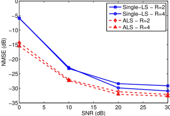
Figure 1: NMSE versus SNR forR=2 andR=4.
The Single-LS method requires that the following identifiability condition be satisfied:rZ=Q, i.e.ZTis right invertible or
equiva-lentlyZis full column rank. So, another advantage of this approach is that it does not impose constraints on the number of antennas, contrarily to the ALS algorithm and to other methods [4, 6, 7, 8, 18].
6. SIMULATION RESULTS
In this section, the proposed channel estimation algorithms are eval-uated by means of simulations. A MIMO Wiener model of an uplink channel of a ROF multiuser communication system [1, 6] is considered for the simulations. The multipath wireless link is characterized by aR×2 convolutive linear mixer, withT=2 users (Q=4) andRhalf-wavelength spaced receive antennas. The E/O conversion is modeled by the following polynomialc1x+c3|x|2x,
withc1=−0.35 andc3=1 [1, 22]. All the Monte Carlo simulation results were obtained usingNR=100 independent data realizations
and the modulation of the transmitted signals is 8-PSK. The spread-ing codes are complex exponentials with an unitary modulus and a phase uniformly distributed over the set[−π,π].
The performance is evaluated in terms of the Normalized Mean Squared Error (NMSE) of the estimated channel parameters,
de-fined as: NMSE = 1 NR∑
NR
l=1
kG−Gˆlk2F
kGk2
F
, where ˆGl represents the
channel matrix estimated at thelthMonte Carlo simulation. Figure 1 shows the NMSE versus Signal-to-Noise-Ratio (SNR) provided by the ALS and Single-LS algorithms forR=2 and 4, withP=3 andD=5. From these simulation results, we can con-clude that the performance of the proposed estimation methods is not deteriorated in the underdetermined case (R=2), with respect to the overdetermined case (R=4). Moreover, it can be viewed that the ALS algorithm provides better performances than the Single-LS algorithm. However, the Single-LS algorithm has a computational cost significantly smaller. For instance, in Figure 1, forSNR=0dB, the ALS algorithm needs approximatively 6 iterations to converge, with two LS estimate computations per step, while the Single-LS algorithm computes only one LS estimate. For small SNR values andD=3 or 4, the ALS algorithm can take more than 50 iterations to converge.
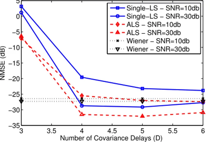
Figure 2 shows the NMSE versus the number of used covari-ance delaysDwith the ALS and Single-LS algorithms forSNR= 10dBandSNR=30dB, withP=3 andR=2. In order to provide a performance reference, we also show the NMSE obtained with the supervised Wiener solution, given by:
ˆ
H=Ryˆ s˜Rˆ− 1 ˜
ss˜, (32)
3 3.5 4 4.5 5 5.5 6 −35
−30 −25 −20 −15 −10 −5 0 5
NMSE (dB)
Number of Covariance Delays (D)
Single−LS − SNR=10db Single−LS − SNR=30db ALS − SNR=10db ALS − SNR=30db Wiener − SNR=10db Wiener − SNR=30db
Figure 2: NMSE versus the number of covariance delays Dfor
SNR=10dBandSNR=30dB.
Ey(n)s˜H(n)andRs˜s˜=E˜s(n)s˜H(n)=IQ,IQbeing the identity
matrix of orderQ. From these simulation results, we can conclude that the accuracy of the ALS estimate does not change significantly forD≥4. Besides, the performance of the two proposed estimation methods is better than that of the supervised Wiener solution for
SNR=30dB. This is due to the fact that the Wiener solution does not exploit the time correlation of the transmitted signals, while the proposed methods do.
7. CONCLUSION
In this paper, we have proposed two new methods for identifying MIMO Volterra communication channels using the PARAFAC de-composition of a tensor composed of channel output covariances, with PSK input signals. This tensor-based approach provides weak uniqueness conditions, leading to weaker constraints on the num-ber of antennas than those imposed by other existing estimation methods. The proposed channel estimation algorithms have been applied for identifying an uplink channel in a ROF multiuser com-munication system. Some simulation results have illustrated the performance of these algorithms, the ALS providing better perfor-mance, at the price of a higher computational cost with respect to the Single-LS algorithm. Both algorithms outperform the Wiener solution for high SNR values.
REFERENCES
[1] S. Z. Pinter and X. N. Fernando, “Estimation of radio-over-fiber uplink in a multiuser CDMA environment using PN spreading codes,” inCanadian Conf. on Elect. and Comp. Eng., May 1-4, 2005, pp. 1–4.
[2] X. N. Fernando and A. B. Sesay, “Higher order adaptive filter based predistortion for nonlinear distortion compensation of radio over fiber links,” inIntern. Conf. on Comm. (ICC), New-Orleans, LA, USA, June 2000, vol. 1/3, pp. 367–371. [3] X. N. Fernando and A. B. Sesay, “A Hammerstein-type
equal-izer for concatenated fiber-wireless uplink,” IEEE Trans. on Vehicular Tech., vol. 54, no. 6, pp. 1980–1991, 2005. [4] A. J. Redfern and G. T. Zhou, “Blind zero forcing equalization
of multichannel nonlinear CDMA systems,” IEEE Trans. on Sig. Proc., vol. 49, no. 10, pp. 2363–2371, Oct. 2001. [5] R. A. Harshman, Foundations of the PARAFAC procedure:
Models and conditions for an “explanatory” multimodal fac-tor analysis, UCLA Working Papers in Phonetics, pp. 1-84, 16thedition, Dec. 1970.
[6] C. A. R. Fernandes, G. Favier, and J. C. M. Mota, “Blind source separation and identification of nonlinear multiuser
channels using second order statistics and modulation codes,” inIEEE Signal Processing Advances in Wireless Communica-tions (SPAWC) workshop, Helsinki, Finland, 17-20 Jun. 2007. [7] G. B. Giannakis and E. Serpedin, “Linear multichannel blind equalizers of nonlinear FIR Volterra channels,” IEEE Trans. on Sig. Proc., vol. 45, no. 1, pp. 67–81, Jan. 1997.
[8] R. Lopez-Valcarce and S. Dasgupta, “Blind equalization of nonlinear channels from second-order statistics,”IEEE Trans. on Sig. Proc., vol. 49, no. 12, pp. 3084–3097, Dec. 2001. [9] R. Bro, Multi-way analysis in the food industry: Models,
al-gorithms and applications, Ph.D. thesis, University of Ams-terdam, AmsAms-terdam, 1998.
[10] N. Petrochilos and K. Witrisal, “Semi-blind source separa-tion for memoryless Volterra channels in UWB and its unique-ness,” inIEEE Workshop on Sensor Array and Multichannel Proc., Waltham, MA, USA, 12-14 Jul. 2006, pp. 566–570. [11] S. Benedetto, E. Biglieri, and R. Daffara, “Modeling and
per-formance evaluation of nonlinear satellite links - A Volterra series approach,” IEEE Trans. on Aerospace Electronic Sys-tems, vol. 15, pp. 494–507, Jul. 1979.
[12] S. Benedetto and E. Biglieri, “Nonlinear equalization of digi-tal satellite channels,”IEEE J. on Select. Areas in Comm., vol. 1, no. 1, pp. 57–62, Jan. 1983.
[13] E. Biglieri, A. Gersho, R. Gitlin, and T. Lim, “Adaptive can-cellation of nonlinear intersymbol interference for voiceband data transmission,”IEEE J. on Select. in Areas Commun., vol. 2, no. 5, pp. 765–777, 1984.
[14] S. Serfaty, J.L. LoCicero, and G.E. Atkin, “Cancellation of nonlinearities in bandpass QAM systems,” IEEE Trans. on Comm., vol. 38, no. 10, pp. 1835–1843, 1990.
[15] C.-H. Cheng and E.J. Powers, “Optimal Volterra kernel esti-mation algorithms for a nonlinear communication system for PSK and QAM inputs,” IEEE Trans. on Sig. Proc., vol. 49, no. 1, pp. 147–163, 2001.
[16] N. D. Sidiropoulos, G. B. Giannakis, and R. Bro, “Blind PARAFAC receivers for DS-CDMA systems,” IEEE Trans. on Sig. Proc., vol. 48, no. 3, pp. 810–823, Mar. 2000. [17] A. Belouchrani, K. Abed-Meraim, J.-F. Cardoso, and
E. Moulines, “A blind source separation technique using second-order statistics,” IEEE Trans. on Sig. Proc., vol. 45, no. 2, pp. 434–444, Feb. 1997.
[18] C. A. R. Fernandes, G. Favier, and J. C. M. Mota, “A mod-ulation code-based blind receiver for memoryless multiuser Volterra channels,” inAsilomar Conference on Signals, Sys-tems, and Computers, Pacific Grove, CA, USA, Nov. 4-7 2007.
[19] C. A. R. Fernandes, G. Favier, and J. C. M. Mota, “Blind estimation of nonlinear instantaneous channels in multiuser CDMA systems with PSK inputs,” inIEEE Signal Processing Advances in Wireless Communications (SPAWC) workshop, Recife, Brazil, Jul. 6-9 2008.
[20] N.D. Sidiropoulos and R. Bro, “On the uniqueness of mul-tilinear decomposition of N-way arrays,” Journal of Chemo-metrics, vol. 14, no. 3, pp. 229–239, 2000.
[21] X. Liu and N.D. Sidiropoulos, “Cramer-Rao lower bounds for low-rank decomposition of multidimensional arrays,” IEEE Trans. on Sig. Proc., vol. 49, no. 9, pp. 2074–2086, Sept. 2001. [22] S. Z. Pinter and X. N. Fernando, “Concatenated fiber-wireless channel identification in a multiuser CDMA environment,”