Journal of Engineering Science and Technology Review 6 (3) (2013) 16-24
Research Article
Input Frequencies Optimization Based on Genetic Algorithm for Maximal Mutual
Information
S. A. Djennas, L. Merad and B. Benadda
Laboratoire de Télécommunications, Faculté de Technologie, Université Abou-Bekr Belkaïd , B. P. 230, Chetouane, Tlemcen (13000), Algérie (Algeria)
.
Received 9 March 2013; Accepted 10 November 2013
___________________________________________________________________________________________
Abstract
Among encountered problems in digital and analog communications, there is mismatch between canals and sources. As regards theory of information, unfortunately, this mismatch found expression in information loss during transfer to reception side. In order to settle the problem, the solution consists in adjustment of probability law at source so that we maximize the mean mutual information. For a little number of symbols, either at emission or at reception, the work can be done analytically with some difficulties. Unfortunately, the problem have tendency to become more and more difficult and complicated as number of symbols increases. In this case and as alternative, we propose a non-traditional optimization method, namely genetic algorithm, which will express, with regard to our problem, all its efficiency through this paper with some conclusive applications.
Keywords:
information theory, entropy, mutual information, channel capacity, optimization, genetic algorithm.
__________________________________________________________________________________________
1. Introduction
In a communication system, we try to convey information from one point to another, very often in a noisy environment.
The question is what is the maximum amount of meaningful information which can be conveyed? This question may not have a definite answer because it is not very well posed. In particular, we do not have a precise measure of meaningful information. Nevertheless, this question is an illustration of the kind of fundamental questions we can ask about a communication system [1]-[5].
Information, which is not a physical entity but an abstract concept, is hard to quantify in general. This is especially the case if human factors are involved when the information is utilized. In other words, we can derive utility from the same information every time in a different way. For this reason, it is extremely difficult to devise a measure which can quantify the amount of information contained in an event.
Shannon introduced two fundamental concepts about information from the communication point of view. First, information is uncertainty. More specifically, if a piece of information we are interested in is deterministic, then it has no value at all because it is already known with no uncertainty. Consequently, an information source is naturally modeled as a random variable or a random process, and probability is employed to develop the theory of information.
Second, information to be transmitted is digital. This means that the information source should first be converted into a stream of 0's and 1's called bits, and the remaining task is to deliver these bits to the receiver correctly with no reference to their actual meaning. This is the foundation of all modern digital communication systems [1]-[5].
In the same work, Shannon also proved two important theorems. The first theorem, called the source coding theorem, introduces entropy as the fundamental measure of information which characterizes the minimum rate of a source code representing an information source essentially free of error. The source coding theorem is the theoretical basis for lossless data compression.
The second theorem, called the channel coding theorem, concerns communication through a noisy channel. It was shown that associated with every noisy channel is a parameter, called the capacity, such that information can be communicated reliably through the channel as long as the information rate is less than the capacity.
These two theorems, which give fundamental limits in point-to-point communication, are the two most important results in information theory.
Shannon's information measures refer to entropy, conditional entropy, mutual information, and conditional mutual information. They are the most important measures of information in information theory [1]-[5].
Now, let us put ourselves in the situation of a transmission system for which the channel is established as a memoryless one. Our purpose through this survey is then, to define the optimal probability law at emission side which will give the maximal mutual information with reception side. For this aim we will use genetic algorithm as
J
estr
JOURNAL OF Engineering Science andTechnology Review
www.jestr.org
______________
* E-mail address: [email protected]
17
optimization process to do the task, but before we will give some basic notions in information theory.
2. Information measures
We begin by introducing the entropy of a random variable. As we will see shortly, all Shannon's information measures can be expressed as linear combinations of entropies. The entropy H (X) of a random variable X is:
H X =− px logp x
!
(1)
The base of the logarithm can be chosen to be any convenient real number greater than 1. When the base of the logarithm is 2, the unit for entropy is the bit.
The definition of the joint entropy of two random variables is similar to the definition of the entropy of a single random variable. The joint entropy H (X, Y) of a pair of random variables X and Y is defined as [1]-[5]:
H X,Y =− p x,y logp x,y
!,!
(2)
For two random variables, we define in the following the conditional entropy of one random variable when the other random variable is given. Fig. 1 shows correspondence between two random variables X and Y.
Fig. 1. Correspondence between two random variables X and Y
Every correspondence is weighted by conditional probability p (yj xi). For random variables X and Y, the
conditional entropy of Y given X is defined as:
H Y X =− p x,y logp y x !,!
(3)
For random variables X and Y, the mutual information between X and Y is defined as [1]-[5]:
I X,Y =− p x,y logp x,y p x p y !,!
(4)
3. Discrete memoryless channels
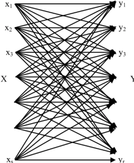
A channel is a communication device with two ends, an input end, or transmitter, and an output end, or receiver. A discrete channel accepts for transmission the characters of some finite alphabet X = {x1,..., xs}, the input alphabet,
and delivers characters of an output alphabet Y = {y1,..., yr}
to the receiver.
Every time an input character is accepted for transmission, an output character subsequently arrives at the receiver.
Let the input alphabet be X = {x1,..., xs}, and the output
alphabet be Y = {y1,..., yr}. By the assumption of
memorylessness, the probability that yj will be received, if xi
is the input character, depends only on i, j, and the nature of the channel. We denote this probability by qij. The qij are
called the transition probabilities of the channel, and the s×r matrix Q = [qij] is the matrix of transition probabilities or
channel matrix. After the input and output alphabets have been agreed upon, Q depends on the channel itself. We could say that Q is a property of the channel. Note that:
Q=
p y! x! ⋯ p y! x!
⋮ ⋱ ⋮
p y! x! ⋯ p y! x!
(5)
With:
q!"= !!!
!!!
p y! x!
!!!
!!!
=1
for each i; that is, the row sums of Q are all 1.
And:
p y! = p y!, x! !!!
!!!
= p y! x!
!!!
!!!
p x! (6)
We have a memoryless channel with input alphabet X, output alphabet Y, and transition probabilities qij. For i ∈
{1,..., s}, let pi denote the relative frequency of transmission,
or input frequency, of the input character xi. In a large
number of situations, it makes sense to think of pi as the
proportion of the occurrences of xi to be transmitted through
the channel.
4. Channel capacity of a discrete memoriless channel
Let a source emit symbols x1, x2,…, xs. The receiver receives
symbols y1, y2,…, yr. The set symbols yj may or may not be
identical to the set xi. With these considerations, we may
write [6]-[8]:
I X,Y = p y!, x! log!p y! x!
p y! !!!
!!! !!!
!!!
After some development, we can write:
Y X
x1
x2
x3
xs
y1
y2
y3
18 IX,Y
= p x! p y! x! log!
p y! x!
p x! p y! x!
!!!
!!!
!!!
!!! !!!
!!!
(7)
The last equation is given in term of input symbol probabilities and channel matrix.
The capacity of a discrete memoryless channel is defined as the maximum of I (X,Y) with respect of p(xi) [7]-[8]:
C=maxIX,Y !!
! (8)
That is:
∂IX,Y
∂p x
! !!!,!,…,!
=0 (9)
Where X and Y are respectively the input and the output of the generic discrete channel, and the maximum is taken over all input distributions p (xi).
We are interested in communication, the transfer of information; it is reasonable to suppose that we ought, therefore, to be interested in the mutual information between the input and output systems. It would be interesting to know the maximum value that I (X, Y) can have. As indicated, that maximum value is called the capacity of the channel, and any values of p1,..., ps for which that value is
achieved are called optimal input (or transmission) frequencies for the channel.
If you accept I (X, Y) as an index, or measure, of the potential effectiveness of communication attempts using this channel, then the capacity is the fragile acme of effectiveness [6]-[8]. This peak is achieved by optimally adjusting the only quantities within our power to adjust, once the hardware has been established and the input alphabet has been agreed to, namely, the input frequencies. The main idea of this section is to show how to find the optimal input frequencies. But before launching into the technical details, let us muse a while on the meaning of what it is that we are optimizing.
The only instances we know of when the optimal input frequencies are not unique are when the capacity of the channel is zero. Certainly, in this case, any input frequencies will be optimal. We conjecture that if the channel capacity is non-zero, then the optimal input frequencies are unique.
The capacity equation is function of both the pi and qij,
supposing there is a solution of the equations at positive pi.
Then for every small wiggle of the qij there will be a positive
solution of the new capacity equations quite close to the solution of the original system.
We can say that there are optimal input frequencies for channel if and only if p1,..., ps satisfy, for some value of C,
the following:
p x!
!!!
!!!
=1
And:
p y! x! log!
p y! x!
p x! p y! x! !!!
!!!
!!!
!!!
=C
Furthermore, if p1,..., ps are optimal input frequencies
satisfying these equations, for some value of C, then C is the channel capacity [1]-[5].
This theorem may seem, at first glance, to be saying that all you have to do to find the capacity of a channel and the optimal input frequencies is to solve the capacity equations of the channel. However, there is a loophole, a possibility that slips through a crack in the wording of the theorem. It is possible that the capacity equations have no solution or no solution with all the pi positive.
Generally, determination of optimal input frequencies is hard work and with no guarantee to find the best solution, especially for great number of inputs and outputs. Consequently, we propose in this paper an alternative for maximization of mutual information, i.e. determination of channel capacity C, based on non-traditional method, namely genetic algorithm. This algorithm doesn’t require any derivative information and do not fail where others do. Moreover, genetic algorithm guarantees good solution, even if it is not the best, with easy possibility to integrate as many constraints as we need. In the next section, we give some basic definitions about this heuristic algorithm. For our purpose and as we will see later, the mutual information I constitutes the fitness, which is the unique link between genetic algorithm and the entire problem.
5. Anatomy of a genetic algorithm
A genetic algorithm (GA) offers an alternative to traditional local search algorithms. It is an optimization algorithm inspired by the well-known biological processes of genetics and evolution. Evolution is closely intertwined with genetics. It results in genetic changes through natural selection, genetic drift, mutation, and migration. Genetics and evolution result in a population that is adapted to succeed in its environment. In other words, the population is optimized for its environment [9]-[17].
A combination of genetics and evolution is analogous to numerical optimization in that they both seek to find a good result within constraints on the variables. Input to objective or cost or fitness function is a chromosome. The output of the objective function is known as the cost when minimizing. Each chromosome consists of genes or individual variables. The genes take on certain alleles much as the variable has certain values. A group of chromosomes is known as a population. For our purposes, the population is a matrix with each row corresponding to a chromosome.
pop=
chrom ! chrom
! ⋮
chrom!
=
gene!! ⋯ gene!"
⋮ ⋱ ⋮
gene!" ⋯ gene!"
Each chromosome is the input to fitness function. The cost associated with each chromosome is calculated by the fitness function.
f
chrom ! chrom
! ⋮
chrom!
= cost
! cost
!
⋮ cost!
19
Often, the numerical values assigned to genes are in binary format. Continuous values have an infinite number of possible combinations of input values, whereas binary values have a very large but finite number of possible combinations of input values. Binary representation is also common when there are a finite number of values for a variable. However, when the variables are continuous, it is more logical to represent them by floating-point numbers. In addition, since the binary GA has its precision limited by the binary representation of variables, using floating point numbers instead easily allows representation to the machine precision [9]-[12].
This continuous GA also has the advantage of requiring less storage than the binary GA because a single floating-point number represents the variable instead of nbits integers. The continuous GA is inherently faster than the binary GA, because the chromosomes do not have to be decoded prior to the evaluation of the cost function.
Although the values are continuous, a digital computer represents numbers by a finite number of bits. When we refer to the continuous GA, we mean the computer uses its internal precision and round-off to define the precision of the value.
The algorithm has the following steps:
1. Create an initial population.
2. Evaluate the fitness of each population member. 3. Invoke natural selection.
4. Select population members for mating. 5. Generate offspring.
6. Mutate selected members of the population. 7. Terminate run if stop criteria or go to step 2 if not.
These steps are shown in the flowchart in Fig. 2.
Fig. 2. Genetic algorithm flowchart
The initial population is the starting matrix of chromosomes. For our case, we have s variables used to calculate the output of the cost or fitness function, and then a chromosome in the initial population consists of s random values assigned to these variables. For N chromosomes, our random population matrix is then of size s N.
The chromosomes are passed to the cost function for evaluation. Each chromosome then has an associated cost. Formulating the cost function is an extremely important step in optimization.
Only the healthiest members of the population are allowed to survive to the next generation. We use two ways to invoke natural selection. The first is to keep m healthy chromosomes and discard the rest. This will be achieved by sorting chromosomes based on their fitness and only m chromosomes are retained. A second approach, called thresholding, keeps all chromosomes that have a cost below a threshold cost value. The chromosomes that survive form the mating pool, or the group of chromosomes from which parents will be selected to create offspring.
The fittest members of the population are assigned the highest probability of being selected for mating. We used two common ways for choosing mates, which are roulette wheel and tournament selection. The population must first be sorted for roulette wheel selection. Each chromosome is assigned a probability of selection on the basis of either its rank in the sorted population or its cost. Rank order selection is the easiest implementation of roulette wheel selection. Chromosomes with low costs have a higher percent chance of being selected than to chromosomes with higher costs. The second approach consists in selection of two groups of chromosomes from the mating pool. The chromosome with the lowest cost in each group becomes a parent. Enough of these tournaments are held to generate the required number of parents. The tournament repeats for every parent needed. Tournament selection works well than roulette wheel.
Offspring can be generated from selected parents in different ways. We combine variable values from the two parents into new variable values in the offspring as:
vo1 = αvp1 + (1 – α) vp2
vo2 = (1 – α) vp1 + α vp2
(10)
with:
α: random number on the interval [0, 1] vo1: value in the offspring 1
vo2: value in the offspring 2
vp1: value in the mother chromosome
vp2: value in the father chromosome
Mutation induces random variations in the population. The mutation rate is the portion of values within a population that will be changed. Mutation for continuous variables can take many different forms. One way is to totally replace the selected mutated value with a new random value. This approach keeps all variable values within acceptable bounds. An alternative is to randomly perturb the chosen variable value. We add a normally distributed random value to the variable selected for mutation. Care must be taken to ensure that the values do not extend outside the limits of the variables.
This generational process is repeated until a termination condition has been reached. Common terminating conditions are:
• Set number of iterations. • Set time reached.
• A cost that is lower than an acceptable minimum.
Initial population
Mutated
population Yes
No
Fitness evaluation
Parents Offspring Keep discard
Parents
Generate offspring
Natural selection
Mating pool
Mutate Done?
Stop criteria
20
• A best solution has not changed after a set number of iterations.
These processes ultimately result in the next-generation population of chromosomes that is different from the initial generation. Generally the average fitness will have increased by this procedure for the population, since only the best chromosomes from the preceding generation are selected for breeding [9]-[17].
6. Results
In this section, we will give some results, certain for comparison with theory, others for calculation code efficiency proof.
6. 1. First application
As one can see on figure, in this first application, we have a ternary symmetric channel with X={x1, x2, x3} and
Y={y1, y2, y3}. The channel matrix is given by:
Q=
1 0 0
0 p 1−p
0 1−p p
With a lot of math and exhaustive calculus, one can deduce that optimal input frequencies are:
p x!
= 1
1+2! !"#! !!!!! !"#! !!!!! 11
p x! =p x! =
1−p x!
2
= 2
! !"#! !!!!! !"#! !!!
1+2! !"#! !!!!! !"#! !!!!! (12)
and the channel capacity:
C=maxIX,Y !!!
C
=log! 1
+2! !"#! !!!!! !"#! !!!!!
(13)
The base for logarithm is 2.
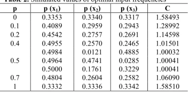
Now we give results of simulation to prove the efficiency of our approach and to validate the calculation code based on genetic algorithm. For different values of p, Tab. 1 resumes theoretical values of input frequencies and channel capacity, while Tab. 2 resumes simulated values.
Table 1. Theoretical values of optimal input frequencies
p p (x1) p (x2) p (x3) C
0 0.3333 0.3333 0.3333 1.5850
0.1 0.4090 0.2955 0.2955 1.2898
0.2 0.4520 0.2740 0.2740 1.1457
0.4 0.4950 0.2525 0.2525 1.0146
0.5 0.5000 0.2500 0.2500 1.0000
0.7 0.4794 0.2603 0.2603 1.0606
1 0.3333 0.3333 0.3333 1.5850
Table 2. Simulated values of optimal input frequencies
p p (x1) p (x2) p (x3) C
0 0.3353 0.3340 0.3317 1.58493
0.1 0.4089 0.2959 0.2943 1.28992
0.2 0.4542 0.2757 0.2691 1.14598
0.4 0.4955 0.2570 0.2465 1.01501
0.5
0.4984 0.0121 0.4885 1.00032
0.4964 0.4741 0.0285 1.00041
0.5000 0.1761 0.3229 1.00041
0.7 0.4804 0.2604 0.2582 1.06090
1 0.3332 0.3336 0.3342 1.58510
Except for p = 0.5, theoretical and simulated values are very close. For p = 0.5, theoretical values are unique but for simulated values there is fluctuation except for p (x1). This
can be explained easily. In fact for p=0.5, any couple of p (x2) and p (x3) have the same impact on value of C. that is
for p = 0.5, we have the minimal value of C and no influence of p (x2) and p (x3) on it. This is why we have swinging
values for p (x2) and p (x3). Of course we have always
p(x2)+p(x3)=1–p(x1)=0.5.
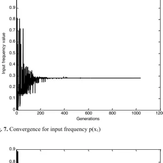
The following figures show convergence, which is evident, for input frequencies and channel capacity through generations.
Fig. 3. Convergence for input frequency p(x1)
0 50 100 150 200 250 300 350 400 450 500
0 0.1 0.2 0.3 0.4 0.5 0.6 0.7 0.8 0.9 1
Generations
In
p
u
t fr
e
q
u
e
n
c
y
v
a
lu
e
Y X
1 - p p
p 1 - p x2
x3 y3
y2 1
21
Fig. 4. Convergence for input frequency p(x2)
Fig. 5. Convergence for input frequency p(x3)
Fig. 6. Convergence for channel capacity
6. 2. Second application
For this second application, we have X={x1, x2, x3, x4, x5}
and Y={y1, y2, y3, y4}. We set the following channel matrix:
Q=
0.48 0.24 0.16 0.12
0.12 0.16 0.24 0.48 0.12 0.48 0.24 0.16
0.16 0.12 0.48 0.24
0.24 0.12 0.16 0.48
For this channel matrix, the obtained optimal input frequencies are:
p (x1) = 0.2820
p (x2) = 0.1113
p (x3) = 0.2609
p (x4) = 0.1939
p (x5) = 0.1510
and the corresponding simulated channel capacity is:
Fig. 7. Convergence for input frequency p(x1)
Fig. 8. Convergence for input frequency p(x2)
0 50 100 150 200 250 300 350 400 450 500
0 0.1 0.2 0.3 0.4 0.5 0.6 0.7 0.8 0.9 1
Generations
In
p
u
t fr
e
q
u
e
n
c
y
v
a
lu
e
0 50 100 150 200 250 300 350 400 450 500
0 0.1 0.2 0.3 0.4 0.5 0.6 0.7 0.8 0.9
Generations
In
p
u
t fr
e
q
u
e
n
c
y
v
a
lu
e
0 50 100 150 200 250 300 350 400 450 500 0
0.2 0.4 0.6 0.8 1 1.2 1.4 1.6
Generations
Ch
a
n
n
e
l
Ca
p
a
c
it
y
0 200 400 600 800 1000 1200
0 0.1 0.2 0.3 0.4 0.5 0.6 0.7 0.8 0.9 1
Generations
In
p
u
t fr
e
q
u
e
n
c
y
v
a
lu
e
0 200 400 600 800 1000 1200
0 0.1 0.2 0.3 0.4 0.5 0.6 0.7 0.8 0.9
Generations
In
p
u
t fr
e
q
u
e
n
c
y
v
a
lu
22
Fig. 9. Convergence for input frequency p(x3)
Fig. 10. Convergence for input frequency p(x4)
C = 0.20865
As usual, the following figures show convergence, which is perfect, for input frequencies and channel capacity through generations.
Fig. 11. Convergence for input frequency p(x5)
Fig. 12. Convergence for channel capacity
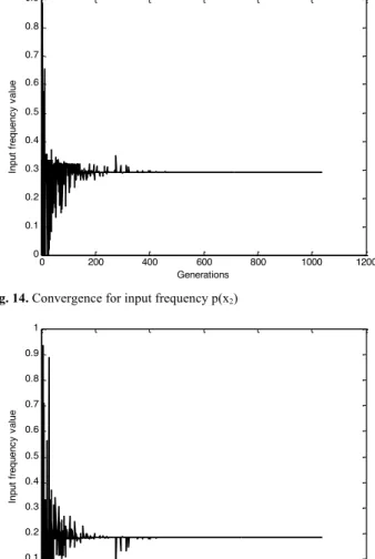
6. 3. Third application
As third application, we take X={x1, x2, x3, x4} for
Y={y1, y2, y3, y4, y5, y6}. The channel matrix is generated
randomly and is given by:
Q
=
0.2808 0.4043 0.0001 0.0013 0.3080 0.0055
0.0478 0.0234 0.6014 0.0189 0.0038 0.3047
0.1911 0.4897 0.0020 0.2655 0.0001 0.0516
0.0001 0.2886 0.0240 0.0000 0.0029 0.6844
The simulated optimal input frequencies are:
p (x1) = 0.3226
p (x2) = 0.2911
p (x3) = 0.1856
p (x4) = 0.1997
and the corresponding channel capacity is:
C = 0.94833
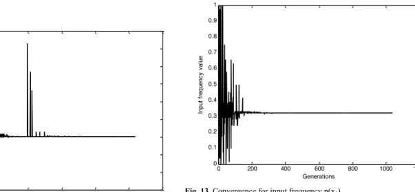
Below and as ever, figures show excellent convergence for input frequencies and channel capacity through generations.
Fig. 13. Convergence for input frequency p(x1)
0 200 400 600 800 1000 1200
0 0.1 0.2 0.3 0.4 0.5 0.6 0.7
Generations
In
p
u
t fr
e
q
u
e
n
c
y
v
a
lu
e
0 200 400 600 800 1000 1200
0 0.1 0.2 0.3 0.4 0.5 0.6 0.7 0.8 0.9
Generations
In
p
u
t fr
e
q
u
e
n
c
y
v
a
lu
e
0 200 400 600 800 1000 1200
0 0.05 0.1 0.15 0.2 0.25 0.3 0.35 0.4 0.45
Generations
In
p
u
t fr
e
q
u
e
n
c
y
v
a
lu
e
0 200 400 600 800 1000 1200
0 0.05 0.1 0.15 0.2 0.25
Generations
Ch
a
n
n
e
l
Ca
p
a
c
it
y
0 200 400 600 800 1000 1200
0 0.1 0.2 0.3 0.4 0.5 0.6 0.7 0.8 0.9 1
Generations
In
p
u
t fr
e
q
u
e
n
c
y
v
a
lu
23
Fig. 14. Convergence for input frequency p(x2)
Fig. 15. Convergence for input frequency p(x3)
Fig. 16. Convergence for input frequency p(x4)
Fig 17. Convergence for channel capacity
7. Conclusion
For efficient transmission, it is necessary to adapt sources to channels. The theory says that we can emit symbols without loss, if information rate is less than the capacity of channel. This parameter is defined as the maximal mutual information between input and output across channel. The mean mutual information is function of input frequencies and the transition probabilities. It is necessary to have measure to this entity, to maximize it and to give assessment about channel by its capacity.
Once the channel is established, the maximization of mutual information is achieved by optimally adjusting the input frequencies. The work is hard and very constraining with much math. To alleviate the procedure, we introduce a genetic algorithm based optimization to bring solution. In fact with this algorithm, there is no need to derivative information and the task is simplified to just formulation of the fitness function, which is the mutual information for our case. This function is the only link between our purpose and genetic algorithm.
The different simulations carried out, show an excellent approach and give very conclusive results. This is very encouraging and constitutes a support to our survey.
______________________________ References
1. C. Arndt, “Information measures”, Springer, 2001.
2. T. M. Cover, J. A. Thomas, “Elements of information theory”, Wiley-Interscience, (2006).
3. I. Csiszár, J. Körner, “Information theory: coding theorems for discrete memoryless systems”, Cambridge University Press, (2011). 4. D. C. Hankerson, G. A. Peter, D. J. Harris, “Introduction to
information theory and data compression”, Chapman and Hall/CRC,
(2003).
5. M. V. Volkenstein, R. G. Burns, A. Shenitzer, “Entropy and information”, Birkhäuser Basel, (2009).
6. I. Land, S. Huettinger, P. A. Hoeher, J. Huber, “Bounds on mutual information for simple codes using information combining”, Annals of Telecommunications, (2004).
7. T. M. Cover, M. Chiang, “Duality between channel capacity and rate
0 200 400 600 800 1000 1200
0 0.1 0.2 0.3 0.4 0.5 0.6 0.7 0.8 0.9
Generations
In
p
u
t fr
e
q
u
e
n
c
y
v
a
lu
e
0 200 400 600 800 1000 1200
0 0.1 0.2 0.3 0.4 0.5 0.6 0.7 0.8 0.9 1
Generations
In
p
u
t fr
e
q
u
e
n
c
y
v
a
lu
e
0 200 400 600 800 1000 1200
0 0.1 0.2 0.3 0.4 0.5 0.6 0.7 0.8 0.9 1
Generations
In
p
u
t fr
e
q
u
e
n
c
y
v
a
lu
e
0 200 400 600 800 1000 1200
0 0.1 0.2 0.3 0.4 0.5 0.6 0.7 0.8 0.9 1
Generations
Ch
a
n
n
e
l
Ca
p
a
c
it
24 distortion with two-sided state information”, IEEE Transactions on
Information Theory, Vol. 48, No. 6, pp. 1629-1638, (2002).
8. G. Caire, S. Shamai, “on the Capacity of some channels with channel state information”, IEEE Transactions on Information Theory, Vol. 45, No. 6, pp. 2007-2019, (1999).
9. R. L. Haupt, S. E. Haupt, “Practical genetic algorithms”, Wiley-Interscience, (2004).
10. C. R. Reeves, J. E. Rowe, “Genetic algorithms - principles and perspectives: a guide to GA theory”, Springer, (2002).
11. S. N. Sivanandam , S. N. Deepa, “Introduction to genetic algorithms”, Springer, (2010).
12. F. Rothlauf, “Representations for genetic and evolutionary algorithms”, Springer, (2010).
13. E. Alba, M.Tomassini, “Parallelism and evolutionary algorithms”, IEEE Transactions on Evolutionary Computation, pp. 443-462, (2002).
14. I. Kushchu, “Genetic programming and evolutionary generalization”, IEEE Transactions on Evolutionary Computation, pp.431-442, (2002).
15. A. Rogers, A. Prugel, “Genetic drift in genetic algorithm selection schemes”, IEEE Transactions on Evolutionary Computation, pp. 298-303, (1999).
16. A. Konaka, D. W. Coitb, A. E. Smith, “Multi-objective optimization using genetic algorithms: A tutorial”, Reliability Engineering and System Safety, pp. 992-1007, (2006).