Quantifying lower tropospheric methane concentrations using near-IR and thermal IR satellite measurements: comparison to the GEOS-Chem model

(1)

AMTD

8, 3851–3882, 2015

Quantifying lower tropospheric

methane concentrations using

Near-IR and Thermal IR satellite measurements

J. R. Worden et al.

Title Page

Abstract Introduction

Conclusions References

Tables Figures

◭ ◮

Back Close

Full Screen / Esc

Printer-friendly Version

Discussion

P

a

per

|

Discussion

P

a

per

|

Discussion

P

a

per

|

Discussion

P

a

per

|

Atmos. Meas. Tech. Discuss., 8, 3851–3882, 2015 www.atmos-meas-tech-discuss.net/8/3851/2015/ doi:10.5194/amtd-8-3851-2015

This discussion paper is/has been under review for the journal Atmospheric Measurement Techniques (AMT). Please refer to the corresponding final paper in AMT if available.

Quantifying lower tropospheric methane

concentrations using near-IR and thermal

IR satellite measurements: comparison to

the GEOS-Chem model

J. R. Worden1, A. J. Turner2, A. A. Bloom1, S. S. Kulawik3, J. Liu1, M. Lee1, R. Weidner1, K. Bowman1, C. Frankenberg1, R. Parker4, and V. H. Payne1

1

Earth Sciences Section, Jet Propulsion Laboratory / CalTech, Pasadena USA

2

School of Engineering and Applied Sciences, Harvard University, Cambridge MA, USA

3

Bay Area Environmental Research Institute, Mountain View CA, USA

4

Deptarment of Physics and Astronomy, University of Leicester, Leicester, UK

Received: 29 March 2015 – Accepted: 3 April 2015 – Published: 20 April 2015

Correspondence to: J. R. Worden (john.worden@jpl.nasa.gov)

Published by Copernicus Publications on behalf of the European Geosciences Union.

(2)

AMTD

8, 3851–3882, 2015

J. R. Worden et al.

Title Page

Tables Figures

◭ ◮

Back Close

Full Screen / Esc

Discussion

P

a

per

|

Discussion

P

a

per

|

Discussion

P

a

per

|

Discussion

P

a

per

|

Abstract

Evaluating surface fluxes of CH4 using total column data requires models to accu-rately account for the transport and chemistry of methane in the free-troposphere and stratosphere, thus reducing sensitivity to the underlying fluxes. Vertical profiles of methane have increased sensitivity to surface fluxes because lower tropospheric

5

methane is more sensitive to surface fluxes than a total column. Resolving the free troposphere from the lower-troposphere also helps to evaluate the impact of trans-port and chemistry uncertainties on estimated surface fluxes. Here we demonstrate the potential for estimating lower tropospheric CH4concentrations through the combi-nation of free-tropospheric methane measurements from the Aura Tropospheric

Emis-10

sion Spectrometer (TES) andXCH4(dry-mole air fraction of methane) from the Green-house Gases Observing Satellite Thermal And Near Infrared for Carbon Observations (GOSAT TANSO, herein GOSAT for brevity). The mean precision of these estimates are calculated to be∼23 ppb for a monthly average on a 4×5 latitude/longitude degree

grid making these data suitable for evaluating lower-tropospheric methane

concentra-15

tions. Smoothing error is approximately 10 ppb or less. The accuracy is primarily deter-mined by knowledge error ofXCO2, used to estimateXCH4from the GOSAT CH4/CO2 “proxy” retrieval. For example, we use differentXCO2fields to quantifyXCH4from the GOSAT CH₄/CO₂ retrieval, one from Carbontracker and another from the NASA Car-bon Monitoring System, and find that differences of up to approximately 60 ppb are

20

possible with a mean value of approximately 35 ppb or less for any given latitude for these lower-tropospheric methane estimates using these two different XCO₂ distribu-tions. We show that these lower-tropospheric concentrations are more directly sensitive to the underlying fluxes than a total column using the GEOS-Chem model. In particular, we compare these lower-tropospheric methane estimates with those from the

GEOS-25

Chem model for July 2009 to determine if these data can capture methane enhance-ments associated with the high-latitude methane fluxes because both TES and GOSAT separately do not show much sensitivity to methane from these sources. We find that

(3)

AMTD

8, 3851–3882, 2015

J. R. Worden et al.

Title Page

Tables Figures

◭ ◮

Back Close

Full Screen / Esc

Discussion

P

a

per

|

Discussion

P

a

per

|

Discussion

P

a

per

|

Discussion

P

a

per

|

the spatial patterns and magnitude of lower tropospheric methane concentrations from GEOS-Chem over Northern European and Siberian wetland fluxes are consistent with these data but modeled concentrations are much larger than measured over Canadian wetland fluxes. Transport of methane significantly affects lower-tropospheric methane concentrations over S.E. Asia as both data and model show methane enhancements

5

that are shifted away from their sources. A possible new finding is that there is no representation of a strong source between the Black and Caspian seas.

1 Introduction

Advances in remote sensing in the last decade have resulted in global mapping of atmospheric methane concentrations (e.g., Frankenberg et al., 2005, 2011; Worden

10

et al., 2012) that in turn have provided new insights into the role of wetlands (e.g., Bloom et al., 2010), fires (e.g., Worden et al., 2012, 2013), the stratosphere (e.g., Xiong et al., 2013), and anthropogenic emissions (e.g. Kort et al., 2014) on tropospheric methane concentrations. However, use of these data to improve global flux estimates and their trends of either methane or CO2, relative to measurements from the surface

15

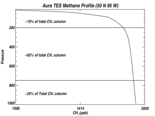
network, is challenging in part because of their measurement accuracy and sampling (e.g., Bergamaschi et al., 2013) or because these measurements are primarily sen-sitive to methane over the whole column or the free-troposphere and stratosphere, which have long mixing length scales (e.g., Keppel-Aleks et al., 2011, 2012; Wecht et al., 2012; Worden et al., 2013). For example, Fig. 1 shows a methane profile derived

20

from Aura Tropospheric Emission Spectrometer (TES) radiances. Because the amount of methane within a sub-column of the profile scales approximately with the pressure di_fference of the layer boundaries, less than 25 % of the total column is typically in the boundary layer where it is most sensitive to the underlying surface fluxes with the remaining column amount in the free-troposphere or stratosphere. Figure 2a and b

25

shows averaged total column measurements derived from GOSAT radiance measure-ments (e.g., Parker et al., 2011 and refs therein) and free-tropospheric measuremeasure-ments

(4)

AMTD

8, 3851–3882, 2015

J. R. Worden et al.

Title Page

Tables Figures

◭ ◮

Back Close

Full Screen / Esc

Discussion

P

a

per

|

Discussion

P

a

per

|

Discussion

P

a

per

|

Discussion

P

a

per

|

from the Aura TES instrument (Worden et al., 2012) for July of 2009 (see Appendix B and Sect. 2.3). Although the total column measurements are more sensitive to near-surface measurements than the TES measurements, both measurements broadly see similar features because they are both strongly sensitive to the bulk of the methane column. The largest methane values occur over the Eastern parts of North America

5

and Asia and moderate values of CH4 over central Asia. Lowest values of the total column are at high-latitudes because the fractional contribution of the depleted strato-sphere to the total column becomes larger with increasing latitude for both data sets. Uncertainties in both of these measurements also increase with latitude because the signal-to-noise of total-column measurements depend on reflected sun-light and the

10

signal-to-noise of thermal infrared based measurements depend on temperature, both of which decrease with increasing latitude. Atmospheric methane concentrations above the lower-troposphere are primarily sensitive to fluxes that are hundreds to thousands of kilometers away, depending on the latitude (e.g., Keppel-Aleks et al., 2011, 2012; Worden et al., 2013). Therefore, uncertainties in transport, both vertical and

horizon-15

tal, are important to consider when using these data to investigate underlying fluxes or processes (e.g., Stephens et al., 2007; Jiang et al., 2013, 2015; Worden et al., 2013).

We next examine the sensitivity of a total column and lower-troposphere column to changes in the underlying fluxes. Figure 3 shows methane fluxes used in Version 9.0.2 of the GEOS-Chem global chemical transport model (Bey et al., 2001; Kaplan

20

et al., 2002; Pickett-Heaps et al., 2011; Wecht et al., 2012, 2014; Turner et al., 2015). Fluxes above 50◦_{N are primarily due to wetlands whereas those at lower latitudes}

are primarily due to a combination of fossil fuels, wetlands, rice-farming, and agricul-ture. Figure 4a shows a comparison between modeledXCH4 above the Hudson Bay Lowlands (∼52◦N, 85◦W) toXCH4, if the modeled southern HBL wetland fluxes are

25

arbitrarily reduced by half. The total column di_fferences in the summer between these two model runs are approximately 10 ppb, about the same as the precision of a single total column measurement from the TANSO GOSAT satellite (Sect. 2). Consequently, substantial averaging and sampling is required to quantify these high-latitude fluxes

(5)

AMTD

8, 3851–3882, 2015

J. R. Worden et al.

Title Page

Tables Figures

◭ ◮

Back Close

Full Screen / Esc

Discussion

P

a

per

|

Discussion

P

a

per

|

Discussion

P

a

per

|

Discussion

P

a

per

|

even to within a factor of two using total column data. In contrast, Fig. 4b shows the effect of this perturbation is much stronger in the lowermost troposphere (the lower-most 250 hPa of atmosphere or approximately surface to 750 hPa) with differences of approximately 40 ppb near the source region. Increasing the sensitivity of remote sens-ing measurements to the underlysens-ing surface fluxes is therefore our motivation for this

5

study. We therefore evaluate the capability of estimating lower tropospheric methane concentrations using GOSAT (SWIR) and TES (TIR) measurements because the com-bination of these measurements provides greater sensitivity to the underlying fluxes and reduced sensitivity to transport error (e.g., Jiang et al., 2015 and refs therein) than either the SWIR or the TIR based measurements alone.

10

2 Estimating lower-tropospheric methane from GOSAT and TES

Recent advances in remote sensing show that combining reflected sunlight and thermal IR measurements to estimate trace gas profiles can provide improved vertical resolu-tion compared to measurements from either individual wavelength region (e.g., Worden et al., 2007, 2010; Kuai et al., 2012). In the case where the trace gas varies

signif-15

icantly in the free-troposphere it is necessary to estimate the trace gas profile from the radiances when the reflected sunlight and thermal IR measurement observe the same air parcel (e.g., Worden et al., 2010). For long-lived trace gases such as CO2 (e.g., Kuai et al., 2012) we can subtract the free-tropospheric/stratospheric posterior estimate (based on thermal IR radiances) from the total column (based on reflected

20

sunlight radiances). In this case observations that are not exactly co-located in space and time can be used together to estimate lower-tropospheric concentrations because of the long mixing length scales of these trace gases in the free-troposphere and strato-sphere (Sect. 3). We therefore use the approach described in Kuai et al. (2012) for es-timating lower tropospheric CO2measurements in which the thermal IR measurement

25

from TES, which provides information about atmospheric methane concentrations from approximately 750 hPa through the stratosphere is subtracted from the total column

(6)

AMTD

8, 3851–3882, 2015

J. R. Worden et al.

Title Page

Tables Figures

◭ ◮

Back Close

Full Screen / Esc

Discussion

P

a

per

|

Discussion

P

a

per

|

Discussion

P

a

per

|

Discussion

P

a

per

|

timates from the GOSAT measurement. For example, Fig. 5 shows an example of the sensitivity of the total column average volume mixing ratio (VMR) of methane from the GOSAT and TES and retrievals (see Appendix B for a summary of the GOSAT and TES retrieval characteristics and data source) respectively to the methane profile (in terms volume mixing ratio or VMR). Both averaging kernels are normalized by the column of

5

each sub-layer (e.g., Eq. 8 in Connor et al., 2008; O’Dell et al., 2012); the GOSAT re-trievals are approximately uniformly sensitive to methane at all levels whereas the TES retrievals have peak sensitivity in the middle/upper troposphere and declining sensitiv-ity towards the surface.

2.1 Estimation approach

10

The retrieved column amount is a function of the prior information, sensitivity, the true state, and uncertainties:

ˆ

C=Ca+CairhTA(x−xa)+Cair

X

i

hT_δ

i. (1)

We define Eq. (1) such that ˆCis the estimated total column in units of molecules cm−2

so that we more conveniently subtract the TES free-tropospheric and stratospheric

col-15

umn amount from the total column amount measured by GOSAT. Theh_{is the column} operator that relates trace gases given in volume mixing ratio (VMR) to the average col-umn mixing ratio (typically given in the literature asXCH₄ for methane), theCair variable is the total dry air column and converts the average column mixing ratio into the dry air column in units of molecules cm−2_{, the}_A_{is the averaging kernel matrix or}_A

=∂_∂xxˆ,

20

wherex_{is the true state and ˆ}_x _{is the estimate of the true state (e.g., Rodgers, 2000).} The superscript “a” refers to the a priori used to constrain the retrieval. The summation overδ refers to all the errors included with this estimate, mapped to a column amount using the “h_{” operator (see Appendix B for summary of the errors in TES and GOSAT} data). Note that the TES data are reported on a log VMR grid. The GOSAT averaging

25

(7)

AMTD

8, 3851–3882, 2015

J. R. Worden et al.

Title Page

Tables Figures

◭ ◮

Back Close

Full Screen / Esc

Discussion

P

a

per

|

Discussion

P

a

per

|

Discussion

P

a

per

|

Discussion

P

a

per

|

a one dimensional vector that is linear in VMR. Both sets of averaging kernels must be converted to the same units prior to comparison.

The GOSAT averaging kernels have been pre-mapped into a “column” averaging kernel,a₌₍hT_A₎_j_/h_j_{, (e.g., Connor et al., 2008) where the subscript “}_j_{” refers to the} pressure levels of the GOSAT retrieval grid. The TES averaging kernels are reported

5

on the forward model pressure levels used in the TES radiative transfer algorithm. For the next set of equations we find it useful to use the nomenclatureb₌hT_A_{which can} be computed from the GOSAT averaging kernels. We next divide up the columns into a lower-tropospheric component (consisting of the pressure levels for the lowermost 250 hPa of the atmosphere or typically surface to 750 hPa), and the rest of the

atmo-10

sphere. The column amount for the lowermost troposphere can then be given as:

ˆ

CL=Cˆtot−CˆU, (2)

where we will use GOSAT to provide the total column and TES to provide the upper tropospheric column (denoted by subscripts tot and U respectively).

Using Eq. (1) we can re-write Eq. (2) as:

15

ˆ

CL=CLa+CairbL xL−xaL

+C_Ua+Cairb G

U xU−xaU

− (3a)

C_Ua+C_Uairh_U_ATES

UU xU−xa_U

+Cair_Uh_U_ATES UL

x_L₋xa L

+Cair

X

i

h_δ_i _(3b)

Equation (3a) represents the GOSAT contribution to the total tropospheric column amount estimate in Eqs. (2) and (3b) represents the TES contribution to the upper tropospheric column. The subscript “L” refers to the pressure levels that make up the

20

“lower troposphere”, the subscript “U” refers to the pressure levels that make up the free-troposphere and stratosphere, the superscript G refers now to the GOSAT averag-ing kernel and the superscript TES refers to the TES averagaverag-ing kernel. The subscripts “UU” and “LL” indicate the block diagonal part of the averaging kernel matrix (A) cor-responding to the “U” and “L” levels, respectively. Because b₌hT_A_{, the vector “}b_U_”

25

(8)

AMTD

8, 3851–3882, 2015

J. R. Worden et al.

Title Page

Tables Figures

◭ ◮

Back Close

Full Screen / Esc

Discussion

P

a

per

|

Discussion

P

a

per

|

Discussion

P

a

per

|

Discussion

P

a

per

|

refers to the “u” set of pressure levels for the vector “b_{” and is not the same as}h_U_A_UU_. Note that we have assumed for the sake of simplicity that the a priori constraint vectors (e.g.,x_a_{) are the same for the GOSAT and TES retrievals as we can always swap one} prior with another (e.g., Rodgers and Connor, 2003). The second part of Eq. (3b) also includes the cross-term “UL” which describes the impact on the upper-tropospheric

5

methane from the lower tropospheric estimate of methane in the TES retrieval (e.g., Worden et al., 2004). We drop this term in subsequent equations as we find it is much smaller than the other error terms. The last term in Eq. (3b) describes the various uncertainties affecting the GOSAT and TES retrievals.

Equation (3) can be re-written as:

10

ˆ

CL=Ca_L+CairbL xL−xa_L

+Cair

b_u_{− ∝}h_u_ATES UU

x_u₋xa_u +X

i

Cihδi, (4)

where_∝₌C_Uair/Cair and the variable Ci in the right side of Eq. (4) refers to either the total column or the upper tropospheric column, depending on the vertical range of the corresponding error.

Typically, data assimilation or inverse estimates of fluxes involve applying the

aver-15

aging kernel from the data to the model, which includes the averaging kernel terms in Eqs. (3a) and (3b). For the comparison discussed in this paper, we will apply Eq. (2) (equivalent to Eq. 4), but without the last term) to the GEOS-Chem model fields. Be-cause the TES and GOSAT instruments do not typically observe the same air-parcel we also must use the approach of subtracting a monthly average of the free-tropospheric

20

CH₄column (based on TES) from the monthly averaged total column based on GOSAT data. This approach will incur a “co-location” error that we evaluate in Sect. 3.1 using the GEOS-Chem model and the TES and GOSAT averaging kernels. A more sophisti-cated approach using both data sets could be to assimilate the TES CH₄fields in order to minimize errors in the model transport and chemistry and then use the GOSAT data

25

to estimate model fluxes (e.g., Kuai et al., 2012); this approach is potentially the subject

(9)

AMTD

8, 3851–3882, 2015

J. R. Worden et al.

Title Page

Tables Figures

◭ ◮

Back Close

Full Screen / Esc

Discussion

P

a

per

|

Discussion

P

a

per

|

Discussion

P

a

per

|

Discussion

P

a

per

|

of a future investigation but is beyond the scope of this current investigation because of the complexities of the data assimilation framework.

2.2 Lower-tropospheric estimates and comparison to GEOS-Chem

We choose to estimate data for July 2009 because (1) both TES and GOSAT have there best overall sampling during this time period and (2) we want to evaluate how

sensi-5

tive these lower-tropospheric estimates are to high-latitude fluxes. Figure 6a shows the July 2009 monthly estimate of XCH4 for the lower troposphere (lowermost 250 hPa of the atmosphere) and Fig. 6b shows the corresponding GEOS-Chem model values after applying the TES and GOSAT averaging kernels, sampling, monthly averaging and subtraction used for the TES and GOSAT lower tropospheric estimate. A global

10

bias of approximately 70 ppb is subtracted from the GEOS-Chem lower tropospheric values; this bias is larger than model/data differences that might be expected from pre-vious studies (e.g., Wecht et al., 2012; Parker et al. 2011; Worden et al., 2012) for the GOSAT and TES retrievals but not unreasonable because the TES data are biased high and the GOSAT data are biased low. The largest near-surface concentrations are

15

in the northern latitudes, as expected by the model (Fig. 6b), and are a result of sum-mertime fluxes of wetlands (e.g., Fig. 3). A combination of biogenic and anthropogenic emissions are responsible for the larger concentrations on the Eastern coasts of North America and Asia with tropical enhancements of methane associated with the source regions in the western Amazon and Congo regions.

20

Figure 7a shows the di_fference between the estimated lower-tropospheric methane and total column with respect to the corresponding GEOS-Chem values. As discussed in the next section, the precision of these data is approximately 23 ppb. Consequently regions that are biased high by 50 ppb or more (red color) or biased low by ₋50 ppb or less (blue colors) are regions where the modeled fluxes are likely in significant

dis-25

agreement with the true fluxes. The largest data/model differences are typically over flux regions (Fig. 3) and suggest that the high-latitude wetland fluxes are too large in the GEOS-Chem model and too low in Europe, North America, and Asia. A large

(10)

AMTD

8, 3851–3882, 2015

J. R. Worden et al.

Title Page

Tables Figures

◭ ◮

Back Close

Full Screen / Esc

Discussion

P

a

per

|

Discussion

P

a

per

|

Discussion

P

a

per

|

Discussion

P

a

per

|

region between the Black and Caspian seas (_∼40◦_{N, 40}◦_{E) is also under-represented}

in the model. For comparison, Fig. 7b shows the total column differences between GOSAT and GEOS-Chem after a global mean bias of∼ −9.5 ppb is removed. As with

Fig. 4, the comparison between Fig. 7a and b empirically demonstrates the increased sensitivity of the lower-tropospheric methane to the underlying methane fluxes as there

5

are significantly larger variations in the lower-tropospheric methane estimates over the larger flux regions. Comparison between Fig. 7a and b also shows how use of the total column alone can lead to erroneous conclusions as the total column data is biased high with respect to the model over South America but the lower-tropospheric estimate comparison shows much more significant variation, with a positive bias in Northern

10

Amazonia and a negative bias in middle Amazonia and Southern Brazil. In addition, the data/model difference for the total column shows very little variation over the Siberian and Northern European wetlands indicating little sensitivity to this important component of the global methane budget.

3 Error analysis

15

We can calculate the “error” statistics of the lower tropospheric methane estimates by subtracting the “true” lower tropospheric column amount (hT

LxL) from Eq. (4) and computing the expectation of this difference:

( ˆCL−CL)( ˆCL−CL) T

=C

2

air(bL−hL)SLL(bL−hL)T

+C_air2 bG

UU− ∝hUATESUU

S_UUbG

UU− ∝hUATESUU

T hT

U+

X

i

C2_ih_S_ihT_, ₍₅₎

20

where theCLis the “true” lower tropospheric column amount and theSi term describes

the statistics (or error covariance) of the error terms “δ” in Eq. (3). The first two terms on the right-hand-side effectively describes the “smoothing error” (Rodgers, 2000) for the lower-tropospheric estimate. A comparison between model (e.g., GEOS-Chem)

(11)

AMTD

8, 3851–3882, 2015

J. R. Worden et al.

Title Page

Tables Figures

◭ ◮

Back Close

Full Screen / Esc

Discussion

P

a

per

|

Discussion

P

a

per

|

Discussion

P

a

per

|

Discussion

P

a

per

|

and data (e.g. GOSAT minus TES) does not need to compare against this smoothing error term as it is removed if the GOSAT and TES averaging kernels are first applied to the model fields. However, we will estimate the smoothing error in the next section (Sect. 3.1) for completeness. Note that there is also a cross-term in this expression that we have ignored because it depends on the atmospheric methane correlations

5

between the upper-troposphere and lower troposphere, which are small, and the term b_L₋h_L_{, which is also small as discussed in next section.}

Uncertainties due to noise and radiative interferences will need to be calculated for any model/data comparison. These errors are contained in the TES and GOSAT prod-uct files as discussed in Worden et al. (2012), Parker et al. (2011) and references

10

therein. The error on the lower-tropospheric column amount will have a much larger percentage error than the total and free-tropospheric estimates for XCH4 because Eq. (2) subtracts two large numbers with similar percentage uncertainties to obtain a smaller number. However, for this comparison we average a month’s worth of data over a 4◦

×5◦ lat/lon grid box, which reduces the random component of this error (e.g.,

15

Worden et al. 2010; Kuai et al. 2012).

We also need to calculate two additional error sources from: (1) the assumption that we can average GOSAT and TES posterior columns on a chosen grid box (in this case 4◦

×5◦) even though the GOSAT and TES observations are not necessarily

co-located and (2) knowledge error of theXCO₂ distribution used to estimate XCH₄

20

concentrations from the GOSAT CH4/CO2“proxy” retrieval.

3.1 Smoothing error from free-troposphere column

The “smoothing error” (Rodgers, 2000) for the lower-tropospheric estimate is given by the first two terms on the right-hand-side of Eq. (5). This term is composed of the smoothing error corresponding to the lowtropospheric levels and the cross state

er-25

ror, which is the impact of the upper-tropospheric estimate on the lower-tropospheric estimate. Both of these errors are removed from any model profile/data comparison if the model is first adjusted with the TES and GOSAT averaging kernels and a

(12)

AMTD

8, 3851–3882, 2015

J. R. Worden et al.

Title Page

Tables Figures

◭ ◮

Back Close

Full Screen / Esc

Discussion

P

a

per

|

Discussion

P

a

per

|

Discussion

P

a

per

|

Discussion

P

a

per

|

ori constraints (or the instrument operators) prior to comparison. However, if only the lower-tropospheric component is compared to the model, in order to model transport and chemistry errors in a data/model comparison, then the second term needs to be included in the overall error budget. We find that the first component of the smoothing error (first term of Eq. 5) is negligible because the expressionb_L₋h_L_{is almost identical}

5

to zero. In fact, this term is approximately 1 ppb even for assumed covariances of up to 200 ppb (squared) in the lower troposphere. We can evaluate the second term (or cross-state error) error an a priori methane climatology from the GEOS-Chem model and the averaging kernels from TES and GOSAT and in general find it to be less than 15 ppb. Note that the TES and GOSAT averaging kernels must both be mapped to the

10

same units and dimensions.

3.2 Co-location error

As discussed previously, most TES and GOSAT observations do not observe the same air parcel; consequently, in order to estimate lower-tropospheric CH₄abundances we subtract monthly averaged free-tropospheric/stratospheric columns (or typically 750

15

to TOA), derived from the TES CH4 profile estimates, from monthly averages of the GOSAT total column:

ˆ

C_LM=CˆM_TOT−CˆM_U, (6)

where the superscript “M” refers to the monthly average. An error results from this as-sumption because the 750–TOA column could change significantly over a month due

20

to transport. For model profile/data comparisons using Eq. (2) or (5), this error is not included in the total error budget because the model is typically sampled at the obser-vations’ spatio-temporal coordinates. However, this error will need to be considered for comparison to monthly averages of aircraft data, for example.

We evaluate this uncertainty by using the GEOS-Chem model and the TES

averag-25

ing kernels. We first calculate the free tropospheric CH4 column (750 hPa to TOA) by

(13)

AMTD

8, 3851–3882, 2015

J. R. Worden et al.

Title Page

Tables Figures

◭ ◮

Back Close

Full Screen / Esc

Discussion

P

a

per

|

Discussion

P

a

per

|

Discussion

P

a

per

|

Discussion

P

a

per

|

applying Eq. (3) to the GEOS-Chem model and using the TES spatio-temporal pling. We then perform the same operation but with the GOSAT spatio-temporal sam-pling and the nearest TES averaging kernels to these spatio-temporal coordinates. We find that the mean RMS difference in the monthly averaged 4◦

×5◦ binned

free-tropospheric sub-column is approximately 7 ppb or less and is effectively random as

5

a function of latitude. We add this uncertainty into the total error budget by computing the RMS of the difference as a function of latitude (Sect. 3.4).

3.3 CO2bias error

The largest potential source of uncertainty in these comparisons is from variable bias error in theXCH4 “proxy” estimates because this estimate of the ratio of CH4to CO2

10

depends on knowledge of the total CO₂ column to infer the CH₄ column (Franken-berg et al., 2010; Butz et al., 2010; Parker et al., 2011). For example, a bias er-ror of 1 % in XCO2 directly leads to a 4 % bias error in the lower-tropospheric sub-column between 1000 and 750 hPa, or approximately 80 ppb for CH₄in the lower tro-posphere. We test the effects of XCO2 knowledge error on our estimates of

lower-15

tropospheric CH4concentrations by first re-normalizing the XCH4 estimates from the GOSAT data (Parker et al., 2013), which usesXCO₂ from the Carbontracker model (Peters et al., 2007), with theXCO₂derived by assimilating GOSAT XCO₂estimates into the land/ocean/atmosphere global carbon models developed for the NASA Car-bon Monitoring System or CMS (e.g, Liu et al., 2014). The revised estimate using the

20

updatedXCO₂ from the CMS results, minus a 20 ppb global bias, is shown in Fig. 8 and shows similar overall variations but also key differences. For example, the Congo region shows higher concentrations of methane and is now more consistent with the GEOS-Chem model. Larger concentrations appear on the East Coast of the USA and China as well as the southern part of the Hudson Bay lowlands. Figure 9 shows the

25

difference between these two lower troposphericXCH4estimates (Fig. 8 vs. Fig. 6a) as a function of latitude. These di_fferences show a mean bias of approximately less than 1 ppb in the southern Tropics and increasing up to approximately 35 ppb in the northern

(14)

AMTD

8, 3851–3882, 2015

J. R. Worden et al.

Title Page

Tables Figures

◭ ◮

Back Close

Full Screen / Esc

Discussion

P

a

per

|

Discussion

P

a

per

|

Discussion

P

a

per

|

Discussion

P

a

per

|

mid-latitudes with maximum values of approximately 60 ppb possible. As a function of latitude, the RMS of the difference ranges from approximately 5 to 20 ppb. We con-servatively add this RMS into the precision part of the error budget. Based on these results, we propose that XCO₂ estimates derived by assimilating data from GOSAT (or from the recently launched Orbiting Carbon Observatory-2 or OCO-2) directly into

5

a global transport model, and then evaluated with aircraft and total column data, have the potential for greatly increasing the accuracy of both the total column and lower tropospheric methane estimates from GOSAT.

3.4 Accuracy and precision

The precision of these estimates can be calculated from the sum of the observation

10

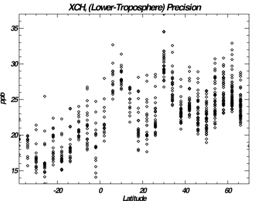
error covariances (noise and spectral interferences), the co-location error, cross-state error, and the RMS of theXCO2error. The observation covariances for a monthly av-erage in each grid box is effectively reduced relative to a single measurement by the square root of the number of observations. The accuracy is primarily determined by knowledge of XCO2 used for the GOSAT XCH4 retrievals. Figure 10 shows the

pre-15

cision function of latitude. The mean precision is approximately 23 ppb with a slight increase from lower to higher latitudes. This precision is sufficient to resolve, for ex-ample, the high-latitude lower-tropospheric concentrations over the Siberian wetlands from the adjacent Russian boreal forest as well as the Canadian wetlands. The ac-curacy could be as large as 35 ppb as shown in Fig. 9 if we use the mean latitudinal

20

di_fference or up to 60 ppb if we use the maximum di_fference. This variation in the accu-racy could have a strong impact on global methane flux inversions as the model would have to balance any large scale methane discrepancies by adjusting the flux.

(15)

AMTD

8, 3851–3882, 2015

J. R. Worden et al.

Title Page

Tables Figures

◭ ◮

Back Close

Full Screen / Esc

Discussion

P

a

per

|

Discussion

P

a

per

|

Discussion

P

a

per

|

Discussion

P

a

per

|

4 Conclusions

This study shows the potential for estimating lower-tropospheric methane concentra-tions using a combination of thermal IR and reflected sunlight measurements. Here we report monthly averaged lower tropospheric methane concentrations (lowermost 250 hPa of the atmosphere) for July 2009 on a 4◦

×5◦ grid. The spatio-temporal

res-5

olution is driven by the sampling of the TES and GOSAT instruments. The smoothing error is approximately 10 ppb or less and the mean precision at this spatio-temporal resolution is approximately 23 ppb. The accuracy of the estimate is primarily due to knowledge error of theXCO2 columns used to quantify XCH4 in the GOSAT “proxy” retrieval.

10

While both TES and GOSAT methane retrievals have been validated against aircraft (Wecht et al. 2012, 2014; Worden et al. 2012; Turner et al., 2015) and up-looking FTS measurements (Parker et al. 2011), it is desirable to validate these lower-tropospheric estimates against aircraft and ground data. However, a robust assessment of these data against ground and aircraft data is beyond the scope of this paper and will

there-15

fore be the subject of a future study. For this reason, we report comparison of these new data against measurements in a future paper. In addition, the GOSATXCH4proxy retrievals should be evaluated using updatedXCO2 columns such as those from the GOSAT or more currently the OCO-2 “Full Physics”XCO₂measurements to potentially improve the accuracy and precision of these data as any bias errors in the total

col-20

umn lead to almost a four-fold increase in the error in the lower-tropospheric methane estimates.

Both the GEOS-Chem model and these new lower tropospheric methane estimates broadly show the same features, which in most cases corresponds to the underlying fluxes specified for the model. However, model/data differences are larger than the

25

calculated errors for Northern Canada, South East Asia, the tropical wetlands, and a region between the Black and Caspian Seas; these regions should be the subject of a future study.

(16)

AMTD

8, 3851–3882, 2015

J. R. Worden et al.

Title Page

Tables Figures

◭ ◮

Back Close

Full Screen / Esc

Discussion

P

a

per

|

Discussion

P

a

per

|

Discussion

P

a

per

|

Discussion

P

a

per

|

The current approach can resolve lower-tropospheric concentrations at monthly time scales on a 4×5 grid. However, many of the key processes controlling wetland fluxes

such as rainfall, flooding, or the freeze and thaw of snow and ice occur at time-scales of much less than a month and at finer spatial scales (e.g., Bloom et al., 2012; Melton et al., 2013; Kort et al., 2014 and many references therein). Consequently it is desirable

5

for an instrument designed to characterize the processes controlling methane to jointly measure the thermal and near-IR radiances for CH4 retrievals at much finer spatial and temporal resolution. A Geo-orbiting satellite with a combined thermal and near-IR capability would greatly improve the spatio-temporal sampling and uncertainty of lower-tropospheric estimates. Combining IR-based CH4measurements from the

Atmo-10

spheric Infrared Sounder (AIRS), Infrared Atmospheric Sounding Interferometer (IASI). IASI, or the Cross-Track Infrared Sounder (CrIS) with total column CH₄ measure-ments from GOSAT or the next-generation Trop-OMI instrumeasure-ments, along with better estimates of total column CO2 from OCO-2 will also greatly enhance our ability to re-solve near-surface methane concentrations, improving sensitivity to estimate methane

15

fluxes, especially at higher latitudes.

Appendix A: Description of GEOS-Chem model

The inputs for the GEOS-Chem model run are described in detail in Picket-Heaps et al. (2011), Worden et al. (2012), Wecht et al. (2014) and Turner et al. (2015). The methane and fire emissions are constrained by the Global Fire Emissions Database

20

(GFED) and the model transport is from re-analysis meteorological fields from the NASA Global Modeling and Assimilation Office. Methane emissions are based on mea-sured emissions factors discussed in Andreae and Merlet (2001) and Van der Werf et al. (2010).

(17)

AMTD

8, 3851–3882, 2015

J. R. Worden et al.

Title Page

Tables Figures

◭ ◮

Back Close

Full Screen / Esc

Discussion

P

a

per

|

Discussion

P

a

per

|

Discussion

P

a

per

|

Discussion

P

a

per

|

Appendix B: Summary of TES and GOSAT retrieval uncertainties

We use Version 6 of the TES CH4data from the “Lite” product files (http://tes.jpl.nasa. gov/data/). A full description of the errors for TES retrievals is provided in Worden et al. (2004) with the basic error analysis theory described in Bowman et al. (2007) and Worden et al. (2012). These errors include the effects of noise as well as radiative

5

interferences from trace gases that absorb and emit in the 8 micron methane band such as H₂O, ozone, and N₂O, as well as the effects of temperature and emissivity.

We use the XCH4 retrievals discussed in Parker et al. (2012). A description of the errors for GOSAT CH4 retrievals is discussed in Butz et al. (2010, 2011), Parker et al. (2012), and Schepers et al. (2012) and references therein and includes the

ef-10

fects of noise, aerosols, and surface albedo. Uncertainties for both the TES and GOSAT retrievals range from 8 to 20 ppb (or 1 % or less). All TES and GOSAT products include uncertainties, the a priori and averaging kernel matrices. In this paper we only derive the uncertainties that result from estimating lower tropospheric methane from combin-ing TES and GOSAT methane retrievals.

15

Acknowledgements. Part of this research was carried out at the Jet Propulsion Laboratory, California Institute of Technology, under a contract with the National Aeronautics and Space Administration. AJT was supported by a Computational Science Graduate Fellowship (CSGF). This research was funded by NASA ROSES CSS proposal 13-CARBON13_2-0071 and the NASA Carbon Monitoring System.

20

References

Andreae, M. O. and Merlet, P.: Emission of trace gases and aerosols from biomass burning, Global Biogeochem. Cy., 15, 955–966, 2001.

Baker, D. F., Bösch, H., Doney, S. C., O’Brien, D., and Schimel, D. S.: Carbon source/sink

information provided by column CO₂measurements from the Orbiting Carbon Observatory,

25

Atmos. Chem. Phys., 10, 4145–4165, doi:10.5194/acp-10-4145-2010, 2010.

(18)

AMTD

8, 3851–3882, 2015

J. R. Worden et al.

Title Page

Tables Figures

◭ ◮

Back Close

Full Screen / Esc

Discussion

P

a

per

|

Discussion

P

a

per

|

Discussion

P

a

per

|

Discussion

P

a

per

|

Bergamaschi, P., Houweling, S., Segers, A., Krol, M., Frankenberg, C., Scheepmaker, R. A., Dlugokencky, E., Wofsy, S. C., Kort, E. A., Sweeney, C., Schuck, T., Brenninkmeijer, C.,

Chen, H., Beck, V., and Gerbig, C.: Atmospheric CH₄ in the first decade of the 21st

cen-tury: inverse modeling analysis using SCIAMACHY satellite retrievals and NOAA surface measurements, J. Geophys. Res.-Atmos., 118, 7350–7369, doi:10.1002/jgrd.50480, 2013.

5

Bey, I., Jacob, D., Yantosca, R., Logan, J., Field, B., Fiore, A., Li, Q., Liu, H. Y., Mickley, L., and Schultz, M. G.: Global modeling of tropospheric chemistry with assimilated meteorology: model description and evaluation, J. Geophys. Res.-Atmos., 106, 23073–23095, 2001. Bloom, A. A., Palmer, P. I., Fraser, A., Reay, D. S., and Frankenberg, C.: Large-scale controls

of methanogenesis inferred from methane and gravity spaceborne data, Science, 327, 322–

10

325, doi:10.1126/science.1175176, 2010.

Bloom, A. A., Palmer, P. I., Fraser, A., and Reay, D. S.: Seasonal variability of tropical wetland

CH₄emissions: the role of the methanogen-available carbon pool, Biogeosciences, 9, 2821–

2830, doi:10.5194/bg-9-2821-2012, 2012.

Bohn, T. J., Lettenmaier, D. P., Sathulur, K., Bowling, L. C., Podest, E., McDonald, K. C., and

15

Friborg, T.: Methane emissions from western Siberian wetlands: heterogeneity and sensitivity to climate change, Environ. Res. Lett., 2, 045015, doi:10.1088/1748-9326/2/4/045015, 2007. Bousquet, P., Ciais, P., Miller, J. B., Dlugokencky, E. J., Hauglustaine, D. A., Prigent, C., Van

Der Werf, G. R., Peylin, P., Brunke, E.-G., Carouge, C., Langenfelds, R. L., Lathière, J., Papa, F., Ramonet, M., Schmidt, M., Steele, L. P., Tyler, S. C., and White, J.: Contribution

20

of anthropogenic and natural sources to atmospheric methane variability, Nature, 443, 439– 443, doi:10.1038/nature05132, 2006.

Bowman, K. W., Rodgers, C. D., Kulawik, S. S., Worden, J., Sarkissian, E., Osterman, G., Steck, T., Lou, M., Eldering, A., and Shephard, M.: Tropospheric emission spectrometer: retrieval method and error analysis, IEEE T. Geosci. Remote, 44, 1297–1307, 2006.

25

Butz, A., Hasekamp, O. P., Frankenberg, C., Vidot, J., and Aben, I.: CH₄retrievals from space-based solar backscatter measurements: performance evaluation against simulated aerosol and cirrus loaded scenes, J. Geophys. Res., 115, D24302, doi:10.1029/2010JD014514, 2010.

Butz, A., Guerlet, S., Hasekamp, O., Schepers, D., Galli, A., Aben, I., Frankenberg, C.,

Hart-30

mann, J. M., Tran, H., Kuze, A., Keppel-Aleks, G., Toon, G., Wunch, D., Wennberg, P., Deutscher, N., Griffith, D., Macatangay, R., Messerschmidt, J., Notholt, J., and Warneke, T.:

(19)

AMTD

8, 3851–3882, 2015

J. R. Worden et al.

Title Page

Tables Figures

◭ ◮

Back Close

Full Screen / Esc

Discussion

P

a

per

|

Discussion

P

a

per

|

Discussion

P

a

per

|

Discussion

P

a

per

|

Toward accurate CO₂and CH₄observations from GOSAT, Geophys. Res. Lett., 38, L14812,

doi:10.1029/2011GL047888, 2011.

Frankenberg, C., Meirink, J., Van Weele, M., Platt, U., and Wagner, T.: Assessing methane emissions from global space-borne observations, Science, 308, 1010–1014, doi:10.1126/science.1106644, 2005.

5

Frankenberg, C., Aben, I., Bergamaschi, P., Dlugokencky, E. J., van Hees, R., Houweling, S., van der Meer, P., Snel, R., and Tol, P.: Global column-averaged methane mixing ratios from 2003 to 2009 as derived from SCIAMACHY: trends and variability, J. Geophys. Res., 116, D04302, doi:10.1029/2010JD014849, 2011.

Gurney, K., Law, R., Denning, A., Rayner, P., Baker, D., Bousquet, P., Bruhwiler, L., Chen, Y.,

10

Ciais, P., and Fan, S.: Towards robust regional estimates of CO₂ sources and sinks using

atmospheric transport models, Nature, 415, 626–630, 2002.

Jiang, Z., Jones, D. B. A., Worden, H. M., Deeter, M. N., Henze, D. K., Worden, J., Bow-man, K. W., Brenninkmeijer, C. A. M., and Schuck, T. J.: Impact of model errors in convective transport on CO source estimates inferred from MOPITT CO retrievals, J. Geophys.

Res.-15

Atmos., 118, 2073–2083, doi:10.1002/jgrd.50216, 2013.

Kaplan, J. O.: Wetlands at the Last Glacial Maximum: distribution and methane emissions, Geophys. Res. Lett., 29, 1079, doi:10.1029/2001GL013366, 2002.

Keppel-Aleks, G., Wennberg, P. O., and Schneider, T.: Sources of variations in total column carbon dioxide, Atmos. Chem. Phys., 11, 3581–3593, doi:10.5194/acp-11-3581-2011, 2011.

20

Keppel-Aleks, G., Wennberg, P. O., Washenfelder, R. A., Wunch, D., Schneider, T., Toon, G. C., Andres, R. J., Blavier, J.-F., Connor, B., Davis, K. J., Desai, A. R., Messerschmidt, J., Notholt, J., Roehl, C. M., Sherlock, V., Stephens, B. B., Vay, S. A., and Wofsy, S. C.: The imprint of surface fluxes and transport on variations in total column carbon dioxide, Biogeo-sciences, 9, 875–891, doi:10.5194/bg-9-875-2012, 2012.

25

Kort, E. A., Frankenberg, C., and Costigan, K. R.: Four corners: the largest

US methane anomaly viewed from space, Geophys. Res. Lett., 41, 6898–6903, doi:10.1002/2014GL061503, 2014.

Kuai, L., Worden, J., Kulawik, S., Bowman, K., Lee, M., Biraud, S. C., Abshire, J. B., Wofsy, S. C., Natraj, V., Frankenberg, C., Wunch, D., Connor, B., Miller, C., Roehl, C., Shia, R.-L., and

30

Yung, Y.: Profiling tropospheric CO₂using Aura TES and TCCON instruments, Atmos. Meas.

Tech., 6, 63–79, doi:10.5194/amt-6-63-2013, 2013.

(20)

AMTD

8, 3851–3882, 2015

J. R. Worden et al.

Title Page

Tables Figures

◭ ◮

Back Close

Full Screen / Esc

Discussion

P

a

per

|

Discussion

P

a

per

|

Discussion

P

a

per

|

Discussion

P

a

per

|

Kulawik, S. S., Jones, D. B. A., Nassar, R., Irion, F. W., Worden, J. R., Bowman, K. W., Machida, T., Matsueda, H., Sawa, Y., Biraud, S. C., Fischer, M. L., and Jacobson, A. R.:

Characterization of Tropospheric Emission Spectrometer (TES) CO₂ for carbon cycle

sci-ence, Atmos. Chem. Phys., 10, 5601–5623, doi:10.5194/acp-10-5601-2010, 2010.

Liu, J., Bowman, K. W., Lee, M., Henze, D. K., Bousserez, N., Brix, H., Collatz, G. J.,

Mene-5

menlis, D., Ott, L., Pawson, S., Jones, D., and Nassar, R.: Carbon monitoring system flux

estimation and attribution: impact of ACOS-GOSATXCO₂sampling on the inference of

ter-restrial biospheric sources and sinks, Tellus B, 66, 22486, doi:10.1117/1.2898457, 2014. Melton, J. R., Wania, R., Hodson, E. L., Poulter, B., Ringeval, B., Spahni, R., Bohn, T.,

Avis, C. A., Beerling, D. J., Chen, G., Eliseev, A. V., Denisov, S. N., Hopcroft, P. O.,

Let-10

tenmaier, D. P., Riley, W. J., Singarayer, J. S., Subin, Z. M., Tian, H., Zürcher, S., Brovkin, V., van Bodegom, P. M., Kleinen, T., Yu, Z. C., and Kaplan, J. O.: Present state of global wetland extent and wetland methane modelling: conclusions from a model inter-comparison project (WETCHIMP), Biogeosciences, 10, 753–788, doi:10.5194/bg-10-753-2013, 2013.

O’Dell, C. W., Connor, B., Bösch, H., O’Brien, D., Frankenberg, C., Castano, R., Christi, M.,

15

Eldering, D., Fisher, B., Gunson, M., McDuffie, J., Miller, C. E., Natraj, V., Oyafuso, F.,

Polon-sky, I., Smyth, M., Taylor, T., Toon, G. C., Wennberg, P. O., and Wunch, D.: The ACOS CO₂

retrieval algorithm – Part 1: Description and validation against synthetic observations, Atmos. Meas. Tech., 5, 99–121, doi:10.5194/amt-5-99-2012, 2012.

Ott, L. E., Pawson, S., Collatz, G. J., Gregg, W. W., Menemenlis, D., Brix, H., Rousseaux, C. S.,

20

Bowman, K. W., Liu, J., and Eldering, A.: Assessing the magnitude of CO₂flux uncertainty in

atmospheric CO₂records using products from NASA’s Carbon Monitoring Flux Pilot Project,

J. Geophys. Res.-Atmos., 120, 734–765, doi:10.1002/(ISSN)2169-8996, 2015.

Parker, R., Boesch, H., Cogan, A., Fraser, A., Feng, L., Palmer, P. I., Messerschmidt, J.,

Deutscher, N., Griffith, D. W. T., Notholt, J., Wennberg, P. O., and Wunch, D.: Methane

25

observations from the Greenhouse Gases Observing SATellite: comparison to ground-based TCCON data and model calculations, Geophys. Res. Lett., 38, L15807, 38, doi:10.1029/2011GL047871, 2011.

Peters, W., Jacobson, A. R., Sweeney, C., Andrews, A. E., Conway, T. J., Masarie, K., Miller, J. B., Bruhwiler, L. M., Pétron, G., and Hirsch, A. I.: An atmospheric perspective

30

on North American carbon dioxide exchange: CarbonTracker, P. Natl. Acad. Sci. USA, 104, 18925–18930, 2007.

(21)

AMTD

8, 3851–3882, 2015

J. R. Worden et al.

Title Page

Tables Figures

◭ ◮

Back Close

Full Screen / Esc

Discussion

P

a

per

|

Discussion

P

a

per

|

Discussion

P

a

per

|

Discussion

P

a

per

|

Pickett-Heaps, C. A., Jacob, D. J., Wecht, K. J., Kort, E. A., Wofsy, S. C., Diskin, G. S., Wor-thy, D. E. J., Kaplan, J. O., Bey, I., and Drevet, J.: Magnitude and seasonality of wetland methane emissions from the Hudson Bay Lowlands (Canada), Atmos. Chem. Phys., 11, 3773–3779, doi:10.5194/acp-11-3773-2011, 2011.

Rodgers, C. D. and Connor, B. J.: Intercomparison of remote sounding instruments, J. Geophys.

5

Res.-Atmos., 108, 4116, doi:10.1029/2002JD002299, 2003.

Schepers, D., Guerlet, S., Butz, A., Landgraf, J., Frankenberg, C., Hasekamp, O., Blavier, J. F., Deutscher, N. M., Griffith, D. W. T., Hase, F., Kyro, E., Morino, I., Sherlock, V., Sussmann, R., and Aben, I.: Methane retrievals from Greenhouse Gases Observing Satellite (GOSAT) shortwave infrared measurements: performance comparison of proxy and physics retrieval

10

algorithms, J. Geophys. Res., 117, D10307, doi:10.1029/2012JD017549, 2012.

Stephens, B. B., Gurney, K. R., Tans, P. P., Sweeney, C., Peters, W., Bruhwiler, L., Ciais, P., Ramonet, M., Bousquet, P., Nakazawa, T., Aoki, S., Machida, T., Inoue, G., Vinnichenko, N., Lloyd, J., Jordan, A., Heimann, M., Shibistova, O., Langenfelds, R. L., Steele, L. P., Francey, R. J., and Denning, A. S.: Weak northern and strong tropical

15

land carbon uptake from vertical profiles of atmospheric CO₂, Science, 316, 1732–1735,

doi:10.1126/science.1137004, 2007.

Turner, A. J., Jacob, D. J., Wecht, K. J., Maasakkers, J. D., Biraud, S. C., Boesch, H.,

Bowman, K. W., Deutscher, N. M., Dubey, M. K., Griffith, D. W. T., Hase, F., Kuze, A.,

Notholt, J., Ohyama, H., Parker, R., Payne, V. H., Sussmann, R., Velazco, V. A., Warneke, T.,

20

Wennberg, P. O., and Wunch, D.: Estimating global and North American methane emissions with high spatial resolution using GOSAT satellite data, Atmos. Chem. Phys. Discuss., 15, 4495–4536, doi:10.5194/acpd-15-4495-2015, 2015.

van der A, R. J., Peters, D. H. M. U., Eskes, H., Boersma, K. F., Van Roozendael, M., De Smedt, I., and Kelder, H. M.: Detection of the trend and seasonal variation in tropospheric

25

NO₂over China, J. Geophys. Res., 111, D12317, doi:10.1029/2005JD006594, 2006.

Wecht, K. J., Jacob, D. J., Wofsy, S. C., Kort, E. A., Worden, J. R., Kulawik, S. S., Henze, D. K., Kopacz, M., and Payne, V. H.: Validation of TES methane with HIPPO aircraft observations: implications for inverse modeling of methane sources, Atmos. Chem. Phys., 12, 1823–1832, doi:10.5194/acp-12-1823-2012, 2012.

30

Wecht, K. J., Jacob, D. J., Sulprizio, M. P., Santoni, G. W., Wofsy, S. C., Parker, R., Bösch, H., and Worden, J.: Spatially resolving methane emissions in California: constraints from the Cal-Nex aircraft campaign and from present (GOSAT, TES) and future (TROPOMI, geostationary)

(22)

AMTD

8, 3851–3882, 2015

J. R. Worden et al.

Title Page

Tables Figures

◭ ◮

Back Close

Full Screen / Esc

Discussion

P

a

per

|

Discussion

P

a

per

|

Discussion

P

a

per

|

Discussion

P

a

per

|

satellite observations, Atmos. Chem. Phys., 14, 8173–8184, doi:10.5194/acp-14-8173-2014, 2014.

Worden, J., Kulawik, S., Shepard, M., Clough, S., Worden, H., Bowman, K., and Goldman, A.: Predicted errors of tropospheric emission spectrometer nadir retrievals from spectral window selection, J. Geophys. Res., 109, D09308, doi:10.1029/2004JD004522, 2004.

5

Worden, J., Liu, X., Bowman, K., Chance, K., Beer, R., Eldering, A., Gunson, M., and Wor-den, H.: Improved tropospheric ozone profile retrievals using OMI and TES radiances, Geo-phys. Res. Lett., 34, L01809, doi:10.1029/2006GL027806, 2007.

Worden, J., Kulawik, S., Frankenberg, C., Payne, V., Bowman, K., Cady-Peirara, K., Wecht, K., Lee, J.-E., and Noone, D.: Profiles of CH₄, HDO, H₂O, and N₂O with improved lower

tro-10

pospheric vertical resolution from Aura TES radiances, Atmos. Meas. Tech., 5, 397–411, doi:10.5194/amt-5-397-2012, 2012.

Worden, J., Jiang, Z., Jones, D. B. A., Alvarado, M., Bowman, K., Frankenberg, C., Kort, E. A., Kulawik, S. S., Lee, M., Liu, J., Payne, V., Wecht, K., and Worden, H.: El Nino, the 2006 Indonesian Peat Fires, and the distribution of atmospheric methane, Geophys. Res. Lett.,

15

40, 4938–4943, doi:10.1002/grl.50937, 2013a.

Worden, J., Wecht, K., Frankenberg, C., Alvarado, M., Bowman, K., Kort, E., Kulawik, S., Lee, M., Payne, V., and Worden, H.: CH₄and CO distributions over tropical fires during Oc-tober 2006 as observed by the Aura TES satellite instrument and modeled by GEOS-Chem, Atmos. Chem. Phys., 13, 3679–3692, doi:10.5194/acp-13-3679-2013, 2013b.

20

Xiong, X., Barnet, C., Maddy, E., Wofsy, S. C., Chen, L., Karion, A., and Sweeney, C.: De-tection of methane depletion associated with stratospheric intrusion by atmospheric infrared sounder (AIRS), Geophys. Res. Lett., 40, 2455–2459, doi:10.1002/grl.50476, 2013.

(23)

AMTD

8, 3851–3882, 2015

J. R. Worden et al.

Title Page

Tables Figures

◭ ◮

Back Close

Full Screen / Esc

Discussion

P

a

per

|

Discussion

P

a

per

|

Discussion

P

a

per

|

Discussion

P

a

per

|

Figure 1.A retrieved methane profile from the Aura TES instrument. The horizontal solid lines are located at 200 and 750 hPa respectively. The region between 1000 to 750 hPa represents the typical pressure range used to define the lower troposphere in this paper.

(24)

AMTD

8, 3851–3882, 2015

J. R. Worden et al.

Title Page

Tables Figures

◭ ◮

Back Close

Full Screen / Esc

Discussion

P

a

per

|

Discussion

P

a

per

|

Discussion

P

a

per

|

Discussion

P

a

per

|

TES 750 hPa - TOA (July 2009)

-100 0 100

Longitude -40

-20 0 20 40 60 80

Latitude

1700 1720 1740 1760 1780 1800 1820 1840

CH

4

PPB

GOSAT Total Column (July 2009)

-100 0 100

-20 0 20 40 60 80

Latitude

1700 1720 1740 1760 1780 1800 1820 1840

CH

4

PPB

(a)

(b)

Figure 2. (a)XCH₄from the GOSAT instrument. Black represents no data.(b)XCH₄from the Aura TES instrument for the free-troposphere to stratosphere (typically 750 hPa to TOA).

(25)

AMTD

8, 3851–3882, 2015

J. R. Worden et al.

Title Page

Tables Figures

◭ ◮

Back Close

Full Screen / Esc

Discussion

P

a

per

|

Discussion

P

a

per

|

Discussion

P

a

per

|

Discussion

P

a

per

|

GEOS-Chem Methane Fluxes

-100 0 100

-20 0 20 40 60 80

Latitude

0 1 2 3 4 5

10

-9 Mols CH

4

m

-2 s

-1

Figure 3.Methane Fluxes used in GEOS-Chem model.

(26)

AMTD

8, 3851–3882, 2015

J. R. Worden et al.

Title Page

Tables Figures

◭ ◮

Back Close

Full Screen / Esc

Discussion

P

a

per

|

Discussion

P

a

per

|

Discussion

P

a

per

|

Discussion

P

a

per

|

Figure 4. (a)Difference inXCH₄between a reference GEOS-Chem run and another in which

the Hudson Bay Lowland Flux has been reduced by half.(b)Same as in(a)but for the lower

troposphere.

(27)

AMTD

8, 3851–3882, 2015

J. R. Worden et al.

Title Page

Tables Figures

◭ ◮

Back Close

Full Screen / Esc

Discussion

P

a

per

|

Discussion

P

a

per

|

Discussion

P

a

per

|

Discussion

P

a

per

|

Normalized TES and GOSAT Averaging Kernels

0.0 0.5 1.0 1.5 2.0

Averaging Kernel 1000

800 600 400 200

Pressure

TES

GOSAT

Figure 5. Sensitivity (or averaging kernel) of the total column with respect to the retrieved GOSAT and TES methane profile. Both averaging kernels have been normalized by the sub-column of each layer in the profile.

(28)

AMTD

8, 3851–3882, 2015

J. R. Worden et al.

Title Page

Tables Figures

◭ ◮

Back Close

Full Screen / Esc

Discussion

P

a

per

|

Discussion

P

a

per

|

Discussion

P

a

per

|

Discussion

P

a

per

|

Figure 6. (a)CH₄ Lower tropospheric estimate using GOSAT and TES data.(b)Lower tropo-spheric estimate from GEOS-Chem model. A mean bias of 70 ppb is removed to better match with the GOSAT/TES data in(a).