www.atmos-chem-phys.net/11/3773/2011/ doi:10.5194/acp-11-3773-2011
© Author(s) 2011. CC Attribution 3.0 License.
Atmospheric
Chemistry
and Physics
Magnitude and seasonality of wetland methane emissions from the
Hudson Bay Lowlands (Canada)
C. A. Pickett-Heaps1,*, D. J. Jacob1, K. J. Wecht1, E. A. Kort1, S. C. Wofsy1, G. S. Diskin2, D. E. J. Worthy3, J. O. Kaplan4, I. Bey5, and J. Drevet6
1School of Engineering and Applied Sciences & Department of Earth and Planetary Sciences, Harvard University,
Cambridge MA 02138, USA
2NASA Langley Research Center, Hampton, Virginia, USA 3Environment Canada, Toronto, Ontario, Canada
4Environmental Engineering Institute, ´Ecole Polytechnique F´ed´erale de Lausanne, Lausanne, Switzerland 5Center for Climate Systems Modeling (C2SM), ETH Z¨urich, Universit¨atstrasse 16, Z¨urich, Switzerland
6Laboratoire de Mod´elisation de Chimie Atmosph´erique, ´Ecole Polytechnique F´ed´erale de Lausanne, Lausanne, Switzerland *current address: CSIRO – Marine and Atmospheric Research, GPO Box 3023, Canberra, ACT, 2601, Australia
Received: 2 August 2010 – Published in Atmos. Chem. Phys. Discuss.: 30 September 2010 Revised: 29 March 2011 – Accepted: 30 March 2011 – Published: 27 April 2011
Abstract. The Hudson Bay Lowlands (HBL) is the second largest boreal wetland ecosystem in the world and an impor-tant natural source of global atmospheric methane. We quan-tify the HBL methane emissions by using the GEOS-Chem chemical transport model to simulate aircraft measurements over the HBL from the ARCTAS and pre-HIPPO campaigns in May–July 2008, together with continuous 2004–2008 sur-face observations at Fraserdale (southern edge of HBL) and Alert (Arctic background). The difference in methane con-centrations between Fraserdale and Alert is shown to be a good indicator of HBL emissions, and implies a sharp sea-sonal onset of emissions in late May (consistent with the air-craft data), a peak in July–August, and a seasonal shut-off in September. The model, in which seasonal variation of emis-sion is mainly driven by surface temperature, reproduces well the observations in summer but its seasonal shoulders are too broad. We suggest that this reflects the suppression of emis-sions by snow cover and greatly improve the model simu-lation by accounting for this effect. Our resulting best esti-mate for HBL methane emissions is 2.3 Tg a−1, several-fold higher than previous estimates (Roulet et al., 1994; Worthy et al., 2000).
Correspondence to:C. A. Pickett-Heaps (christopher.pickett-heaps@csiro.au)
1 Introduction
Methane is the second most important anthropogenic green-house gas after carbon dioxide (IPCC, 2007). Methane concentrations have increased from 700 ppbv in the pre-industrial atmosphere to 1700 ppbv by the early 1990s (Etheridge et al., 1998). This increase is presumably driven by direct emissions from industry and agriculture (IPCC, 2007), but could also reflect changes in the chemical sink (re-action with the OH radical) and the effects of climate change on natural emissions (Worthy et al., 2000). Wetlands are the largest natural source of methane and are highly sensitive to changes in climate (Kaplan et al., 2006), especially in the bo-real zone (Zhuang et al., 2006; Sitch et al., 2007). Here we use aircraft observations over the Hudson Bay Lowlands in northern Ontario as well as surface observations at Fraserdale and Alert to better quantify this boreal wetland source.
The Hudson Bay Lowlands (HBL) is an ecologically significant and well-studied boreal wetlands region (e.g. Glooschenko et al., 1994). It is (after the West Siberian wet-lands) the second largest semi-continuous wetland region in the world, covering an area of 320 000 km2or about 10% of the total area covered by boreal wetlands (Wang et al., 2008; Glooschenko et al., 1994). The ABLE-3B/NOWES airborne and ground campaign conducted in the summer of 1990 esti-mated an annual methane emission of 0.5±0.3 Tg a−1from
the HBL (Roulet et al., 1994). Worthy et al. (2000), using inverse methods to interpret observations from the Alert and Fraserdale Canadian sites, obtained a similar estimate of 0.2– 0.5 Tg a−1. These estimates seem low compared to global inversion studies that infer total boreal wetland emissions of 27–38 Tg a−1 (Hein et al., 1997; Wang et al., 2004; Bous-quet et al., 2006), although Chen and Prinn (2006) obtained an estimate of 7 Tg a−1. Typically, the HBL is assumed to contribute 10% to global boreal wetland emissions.
The above inconsistencies point to the need for a bet-ter understanding of methane emissions from the HBL as a window into the global boreal wetland source. We exploit here methane concentration measurements from the ARC-TAS and Pre-HIPPO aircraft campaigns in May–July 2008 (Fig. 1), together with long-term surface data from Envi-ronment Canada at Fraserdale (81.6◦W, 49.9◦N) and Alert (62.5◦W, 82.5◦N). We interpret these data using a global bottom-up scheme for wetland emissions implemented in the GEOS-Chem chemical transport model (CTM). The ARC-TAS airborne campaign based in Cold Lake, Alberta (Jacob et al., 2010) conducted three flights over the HBL in early July, while the Pre-HIPPO campaign based in Boulder, Col-orado (Pan et al., 2010) conducted 2 flights in the region in May–June.
2 Model description
We use the GEOS-Chem CTM originally described by Bey et al. (2001) in a methane simulation for 2004–2008 to in-terpret the aircraft and surface observations. GEOS-Chem is driven by GEOS-5 analyzed meteorological data from the NASA Global Modeling and Assimilation Office (GMAO). The GEOS-5 data have 1/2◦×2/3◦(lat, lon) horizontal
reso-lution with 72 vertical levels and 6-h temporal resoreso-lution (3-h for surface variables and mixing dept(3-hs). T(3-he (3-horizontal resolution is degraded here to 2◦×2.5◦for input to
GEOS-Chem.
The methane simulation in GEOS-Chem was originally described by Wang et al. (2004), and subsequently improved and updated by Drevet et al. (2011). Major sources in-clude anthropogenic emissions from EDGAR 4.0 (Euro-pean Commission, 2009), natural emissions from wetlands as described below, and GFED2 biomass burning emissions (Giglio et al., 2006). Chemical loss of methane is com-puted using a global 3-D archive of monthly average OH
CH4 flux (2008)
45oN
50oN
55oN
60oN
65oN
110oW 100oW 90oW 80oW 70oW
0 5 10 15 20 g.m-2.a-1
!"#$%&!!'(
((()*+,(-.(/012(3.4(
((()*+,(-5(/678(.54(
9:;<9=(
((()*+,(-.(/67*(->4(
((()*+,(-5(/67*(-?4(
@(A$.(1$3(
)"1B#"C1*#(
!"#$%&"'
()*$+',-./0'123456,' 0#+D18#(EAFBBFG8B(/67*24(
%7CBG8(H12( IGJ*18CB(
)*F@D+(+"1KLB(M(>---A(
Fig. 1.ARCTAS and Pre-HIPPO flight tracks over the Hudson Bay
Lowlands (HBL) below 4 km, superimposed on a map of GEOS-Chem methane emissions for July 2008. The locations of Fraserdale and of the two ABLE-3B/NOWES study regions are also shown. The black rectangle encompasses the HBL region as defined in the present study.
concentrations from a GEOS-Chem simulation of tropo-spheric chemistry. The mean tropotropo-spheric OH concentra-tion is 10.8×10⁵molecules cm−3, typical of current models
(a global model inter-comparison by Shindell et al. (2006) gives a mean value of 11.1±1.7×10⁵molecules cm−3). The corresponding tropospheric lifetime of methylchloro-form against oxidation by OH is 5.3 yr, within the range con-strained by observations (Prinn et al., 2005). Additional mi-nor sinks for methane in the model include stratospheric oxi-dation prescribed as a constant decay (Wang et al., 2004) and soil absorption (from EDGAR 4.0).
The wetlands emission scheme in GEOS-Chem is based on Kaplan (2002). The scheme applies methane emission factors to heterotrophic respiration rates in tropical and bo-real wetlands, following algorithms described by Kaplan et al. (2002), Sitch et al. (2003) and Bergamaschi et al. (2007). The emission flux E (molecules CH4m−2s−1) for each
model grid square is given by:
E=δW FβAe
−E0
T−T0
2 X
i=1 Ci
τi
(1)
where C1 and C2 (mol C m−2) are soil and litter carbon
pools, respectively, specified on a 2◦×2.5◦grid by the
Lund-Potsdam-Jena dynamic global vegetation model (Sitch et al., 2003). These pools have fixed residence times τ1=32 yr
andτ1=2.8 yr from Sitch et al. (2003). The Arrhenius
fac-tor with A=1.0e+3, E0=309 K, and T0=227 K (Lloyd
β=3×10⁻² mol CH4 per mol C respired (Christensen et
al., 1996). An additional scaling factorF is used to match observed ecosystem fluxes of methane, separately for tropi-cal (T) and boreal (B) wetlands:
F=α·FT+(1−α)·FB (2)
where α=min exp ¯
T−T1/8,1, T¯ (K) is the mean
monthly soil temperature taken here as the GEOS-5 skin tem-perature, andT1=303.15 K. Scaling factorsFT=0.14 and FB=0.005 were derived by J. Kaplan and J. Drevet
(per-sonal communication, 2009) to match published emission estimates for the Amazon (Melack et al., 2004) and boreal wetlands (Hein et al., 1997; Wang et al., 2004). Finally,
W in Eq. (1) represents the maximum potential fraction of wetland coverage for the grid square, as obtained from vari-ous databases described by Kaplan et al. (2002) and Berga-maschi et al. (2007). Whether a wetland is actually present (δ=1) or not (δ=0) over that fractionW at any given time depends on the level of the water table, which we diagnose using GEOS-5 soil moisture as a proxy following Bergam-aschi et al. (2007). Wetlands are present if the soil moisture exceeds a specified threshold of 0.1 for the ratio between the soil water content and the porosity of the soil (J. O. K. Ka-plan, personal communication, 2009)
Annual emissions for the HBL (geographically defined as 50◦N–60◦N, 75◦W–96◦W) computed in the above manner in GEOS-Chem average 2.9 Tg a−1for 2004–2008, with the spatial distribution shown in Fig. 1. This estimate is much larger than the previous HBL emission estimates of Roulet et al. (1994) and Worthy et al. (2000).
3 Constraints on HBL methane emissions
We examine the consistency of the GEOS-Chem methane emissions with the aircraft data from Pre-HIPPO and ARC-TAS, and the surface data from Fraserdale and Alert. The DACOM tunable diode laser instrument used in ARCTAS (Sachse et al., 1987) has an estimated accuracy/precision of 1%/0.1%. The quantum cascade laser instrument used in Pre-HIPPO has an estimated accuracy and precision of 0.25%. The surface measurements at Fraserdale are ob-tained by gas chromatography on samples collected from a 40-m high tower and have an accuracy/ precision of 1%/0.2% (Worthy et al., 2003). Similar specifications apply to the sur-face measurements at Alert.
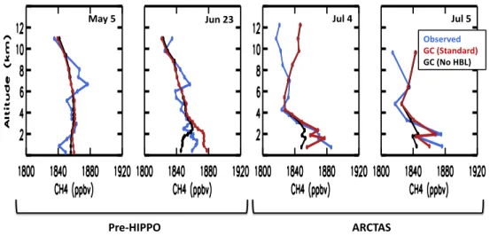
Figure 2 shows the ensemble of aircraft vertical profiles over the HBL from 12 May (Pre-HIPPO) to 5 July (ARC-TAS). We excluded stratospheric air as diagnosed by a molar O3/CO ratio exceeding 1.25 (Hudman et al., 2006) and fire
plumes as diagnosed by CO exceeding 200 ppbv. The lat-ter fillat-ter effectively removed biomass burning influence from the data set as inferred from correlation between methane and CO. The HBL methane enhancements in Fig. 2 can thus be reliably attributed to wetland emissions.
The ARCTAS observations on 4–5 July show strong boundary layer enhancements over the HBL. The Pre-HIPPO flight on 12 May shows no boundary layer enhancement while that on 23 June shows a moderate enhancement. Ob-servers on the Pre-HIPPO aircraft reported snow cover over the HBL on 12 May but not on 23 June. For comparison with the aircraft we sample the model at the time and loca-tion of the flights. We see in Fig. 2 that the model provides a good simulation of the boundary layer structure for the dif-ferent flights, the enhancement observed in ARCTAS, and the sharp springtime transition from May to July. However, model overestimation is evident for the 23 June profile.
To further investigate the magnitude and seasonal on-set of HBL emissions we used 2004–2008 surface data at Fraserdale and Alert collected by Environment Canada, with Alert serving as an Arctic background site against which the HBL influence at the Fraserdale downwind site can be refer-enced (Worthy et al., 1998). For Fraserdale we sample the daily data averaged over the 1700–1900 local time window, when the surface measurements are most representative of a relatively deep mixed layer (Worthy et al., 1998), and further select for surface winds from the northern quadrants, when direct influence from the HBL can be expected (Fig. 1). Se-lection for northerly winds retains∼50% of the original data.
We sample Alert data for the same times at Fraserdale in or-der to facilitate analysis of the difference between the two sites as discussed later.
Figure 3 shows the observed seasonal variations at Fraserdale and Alert for 2004–2008. The observations at Alert show a July minimum due to chemical loss in the Northern Hemisphere. The model minimum lags 4–6 weeks behind, an offset that can be attributed to background error in the seasonal variation of sources, transport, or OH concen-trations. The observations at Fraserdale follow the seasonal variation at Alert in winter-spring but deviate in late May toward an August maximum, ostensibly due to emissions from the HBL. The model shows the same seasonal devia-tion at Fraserdale relative to Alert but shifted 6 weeks early. A model sensitivity simulation with no HBL emissions (also shown in Fig. 3) confirms that the seasonal deviation between Fraserdale and Alert is due primarily to HBL emissions. The model shows multiple seasonal peaks at Fraserdale (late June, late August, early November) compared to a single ob-served peak, but this fine structure reflects fluctuations in the background rather than HBL emissions as discussed below.
!"#$%$ &'($)*$ &'+$,$ &'+$%$
-./01203$ 45$678"(3"139$ 45$6:;$<=>9$
?10@<A??-$ BC5DB7$
Fig. 2. Methane vertical profiles from Pre-HIPPO and ARCTAS over the HBL (May–July 2008). Observations (blue) are compared to
GEOS-Chem (GC) model vertical profiles sampled along the flight tracks at the flight times. The standard simulation (red) and a sensitivity simulation with no HBL emissions (black) are presented.
!!!!!!"!!!!!!!!!#!!!!!!!!$!!!!!!!!%!!!!!!!!$!!!!!!!!"!!!!!!!!!!"!!!!!!!!!!%!!!!!!!!!&!!!!!!!!!'!!!!!!!!(!!!!!!!!)!!
*+
,
!-../
0
1!
Fig. 3. Seasonal variation (2004–2008) of methane at Fraserdale
and Alert. GEOS-Chem results are compared to observations. Also plotted is the model background concentration at Fraserdale as de-rived from a simulation with no HBL emissions. Data are daytime values smoothed with a 28-day moving average and then averaged over 5 yr. For Fraserdale we use only data associated with winds from the northern quadrants.
Figure 4 shows the seasonal variation of the difference in concentrations between Fraserdale and Alert (1CH4),
illus-trating more precisely the methane flux signature from the HBL. Here we assume that Alert provides a reasonable mea-sure of background concentrations at Fraserdale; this is sup-ported in the model by the comparison in Fig. 3 of the model simulation at Alert (thin blue line) and at Fraserdale in the ab-sence of HBL emissions (thick black line). We find that the multi-peak structure of model concentrations at Fraserdale in June–November (Fig. 3) is reduced when corrected for the
!
!"
#
$%
&&'
(
)$
$$$$$$*$$$$$$$$$$+$$$$$$$$$,$$$$$$$$-$$$$$$$$,$$$$$$$$$*$$$$$$$$$$*$$$$$$$$$$-$$$$$$$$$.$$$$$$$$$/$$$$$$$$$0$$$$$$$$1$$
Fig. 4. Mean seasonal differences in CH4concentration between
Fraserdale and Alert (1CH4)for 2004–2008 (data in Fig. 3).
Ob-servations (blue) are compared to the standard GEOS-Chem sim-ulation, a sensitivity simulation restricting emissions to snow-free ground, and a sensitivity simulation with no HBL emissions.
Alert background (Fig. 4). More importantly, we find that any residual multi-peaks in modeled 1CH4 are associated
more with changes in the model background at Fraserdale relative to that at Alert than in HBL model emissions. Tem-poral fluctuations during those two months in the model may also reflect the greater variability in surface temperatures (used in the model to compute methane emission) than in ac-tual soil temperatures. Heat transfer in the soil column would be expected to dampen temporal variability in soil tempera-tures.
observations discussed above and with previous field stud-ies in nearby James Bay peatlands that suggest an onset of emissions in mid-May (Pelletier et al., 2007). By contrast, we see from Fig. 4 that HBL emissions in the model begin in early April. In addition, the observations indicate a sea-sonal shutdown of HBL emissions in September whereas in the model these emissions persist into October. The early on-set of model emissions was not apparent in comparison with the Pre-HIPPO profile on 12 May in Fig. 2, but that is be-cause of delayed spring warming in 2008 and bebe-cause that flight profile sampled the northern edge of the HBL (Fig. 1). The premature onset of HBL methane emissions in the model likely reflects the use of skin temperature as proxy for soil temperature. Seasonal increases in soil temperature at depth lag behind the land surface during the spring thaw. We attempted to impose in the model a time lag for soil heat-ing by usheat-ing the standard heat transport parameterization of Campbell and Norman (1998) with thermal diffusivities from Sitch et al. (2003), but the resulting delay in the onset of emissions was insufficient. Instead we identified persistent snow cover in the GEOS-5 data well past the model onset in model emissions. Snow cover would insulate the underlying soil from warming, inhibiting methanogenesis in spring, and would also trap methane in the autumn (Friborg et al., 1997). Consequently we modified the model to restrict emissions to snow-free regions. Figure 4 shows that this mostly corrects the model biases in the spring and autumn, although there is still a small lag of 1–2 weeks in the spring. This additional delay might reflect a period of time required for the underly-ing peatlands to thaw before methanogenesis ensues (Dunn et al., 2009). Comparison with the aircraft profiles in Fig. 2 is unaffected by the delayed onset in model emissions. The resulting annual reduction in model HBL emissions is 20% (2.3 Tg a−1vs. 2.9 Tg a−1).
The model temporal variability of methane emissions in the snow-free season is driven largely by surface tempera-ture (Eq. 1), and this appears adequate to match the observed July–August maximum of HBL emissions (Fig. 4). Previous studies of boreal wetlands have pointed out the sensitivity of emissions to changes in the level of the water table (Moore et al., 1994; Pelletier et al., 2007). However, the flat topography of the HBL results in poor drainage and maintains persistent wetland coverage throughout the summer.
Figure 5 shows the interannual variation of HBL model emissions for 2004–2008 as driven by temperature and snow cover. The seasonal onset of emission can vary by a month from year to year. There is much less year-to-year variability in the fall shutdown of emissions. The mean annual emission for the 5 yr is 2.3±0.3 Tg a−1.
4 Comparison to ABLE-3B/NOWES estimates
The ABLE-3B/NOWES surface and aircraft field study in July 1990 previously reported an annual emission estimate
!"""""""""""""""#""""""""""""""""!""""""""""""""""""$""""""""""""""""""$""""""""""""""""""#""""""""""""""""""%"""""""""""""""""&""""""""""""""""'"
()
*
"+,-".
/0
"1
234"
526718"971:"
;<<*"
;<<5"
;<<="
;<<>" ;<<?"
;<<*@"""3A?"/0"123"
;<<5@""";A5"/0"123"
;<<=@""";A5"/0"123"
;<<>@""";AB"/0"123"
;<<?@""";A;"/0"123"
Fig. 5. Seasonal variation of HBL methane emissions simulated
by the model for 2004–2008. Values are integrated spatially over
the HBL domain (50◦N–60◦N, 75◦W–96◦W) and smoothed
tem-porally with a 4-week moving average. Also tabulated are annual emission estimates for individual years.
of 0.5±0.2 Tg a−1for the HBL (Harris et al., 1994; Roulet et al., 1994). This is considerably less than our best esti-mate of 2.3 Tg a−1, and would be inconsistent with the Pre-HIPPO and ARCTAS data of Fig. 2 as well as the Fraserdale
1CH4data of Fig. 4. The ABLE-3B/NOWES estimate was
obtained by extrapolation of direct flux measurements at sur-face sites, using wetland coverage derived from satellite and aerial imagery. The surface sites and supporting aircraft eddy correlation flux measurements were located in two small study areas at the southern and northern edges of the HBL (Fig. 1). Roulet et al. (1994) reported mean June-October emission estimates for the southern and northern study ar-eas of 3.4 g m−2a−1 and 6.3 g m−2a−1, respectively, from their surface measurements. Aircraft measurements over these same regions in July yielded consistent mean fluxes of 5±3 g m−2a−1and 4±6 g m−2a−1 respectively. These values agree with our flux estimates of ∼5 g m−2a−1 for both ABLE-3B/NOWES regions in July (Fig. 1). Roulet et al. (1994) went on to infer annual mean emissions by tak-ing their June–October measurements to be representative of free conditions and assuming zero emissions for snow-covered ground. This is consistent with our findings.
The large difference between our estimate of HBL emis-sion estimate and that of Roulet et al. (1994) thus lies in the spatial extrapolation to the scale of the HBL. We see from Fig. 1 that our emissions are much higher in the mid-section of the HBL than in the ABLE-3B/NOWES study regions. The boundary layer methane enhancements observed from the ABLE-3B aircraft (∼30 ppbv) were indeed much lower
5 Conclusions
Aircraft observations over the Hudson Bay Lowlands (HBL) in May–July 2008 show a seasonal onset of methane emis-sions in June and 60 ppbv enhancements in the boundary layer in July. Surface observations at Fraserdale (just south of the HBL), when referenced against a background Arctic site (Alert) to isolate the HBL contribution, indicate a sea-sonal onset of methane emission in late May, a peak emis-sion from mid-July to the end of August, and a sharp de-crease in September. The GEOS-Chem model including a standard methane emission scheme for boreal wetlands can successfully reproduce these observations except for a pre-mature springtime onset and a delayed fall shut-off. Seasonal variation of wetland emission in the model is mainly driven by surface temperature. We find that accounting in addition for suppression of emission by snow cover corrects the model biases in spring and fall. The variability in the model is still larger than observed and this could reflect dampening of soil temperature fluctuations relative to the surface. Our result-ing best estimate of HBL methane emissions is 2.3 Tg a−1, much higher than previous estimates for the region (Roulet et al., 1994; Worthy et al., 2000). We argue that this reflects gradients of methane emission within the HBL that were not previously accounted for.
Acknowledgements. This work was supported by the US National
Science Foundation and by the Tropospheric Chemistry Program of the National Aeronautics and Space Administration. We thank the reviewers for useful comments.
Edited by: A. Stohl
References
Bergamaschi, P., Frankenberg, C., Meirink, J.F., Krol, M., Den-tener, F., Wagner, T., Platt, Y., Kaplan, J.O., Kroner, S., Heimann, M., Dlugokencky, E. J., and Goede, A.: Satellite cartography of atmospheric methane from SCIAMACHY on board ENVISAT: 2. Evaluation based on inverse model simulations, J. Geophys. Res., 112, D02304, doi:10.1029/2006JD007268, 2007.
Bey, I., Jacob, D. J., Yantosca, R. M., Logan, J. A., Field, B. D., Fiore, A. M., Li, Q. B., Lui, H. G. Y., Mickley, L. J., and Schultz, M. G.: Global modeling of tropospheric chemistry with assim-ilated meteorology: Model description and evaluation, J. Geo-phys. Res., 106(D19), 23073–23095, 2001.
Bousquet, P., Ciais, P., Miller, J. B., Dlugokencky, E. J., Hauglus-taine, D. A., Prigent, C., Werf, G. R. Van der, Peylin, P., Brunke, E.-G., Carouge, C., Langenfelds, R. L., Lathiere, J., Papa, F., Ramonet, M., Schmidt, M., Steele, L. P., Tyler, S. C., and White, J.: Contribution of anthropogenic and natural sources to atmospheric methane variability, Nature, 443, 439– 443, doi:10.1038/nature05132, 2006.
Campbell, J. S. and Norman, J. M.: An introduction to Environ-mental Biophysics, 28 pp., Springer, 1998.
Chen, Y. H. and Prinn, R. G.: Estimation of atmospheric methane emissions between 1996 and 2001 using a three-dimensional
global chemical transport model, J. Geophys. Res., 111, D10307, doi:10.1029/2005JD006058, 2006.
Christensen, T. R., Prentice, I. C., Kaplan, J. O., Haxeltine, A., and Sitch, S.: Methane flux from northern wetlands and tundra, Tel-lus, 48, 652–661, doi:10.1034/j.1600-0889.1996.t01-4-00004.x, 1996.
Drevet, J., Bey, I., Kaplan, J., Generoso, G., and Koumoutsaris, S.: A modeling studyof the global methane budget over the period 1990–2004: 1. Model description and evaluation, in preparation, 2011.
Dunn, A. L., Wofsy, S. C., and Bright, A. H.: Landscape het-erogeneity, soil climate, and carbon exchange in a boreal black spruce forest, Ecol. Appl., 19(2), 495–504, 2009.
Etheridge, D. M., Steele, L. P., Francey, R. J., and Langenfelds, R. L.: Atmospheric methane between 1000AD and present: Evi-dence of anthropogenic emissions and climate variability, J. Geo-phys. Res., 103(D13), 15979–15993, 1998.
European Commission, Joint Research Centre (JRC)/Netherlands Environmental Assessment Agency (PBL). Emission Database for Global Atmospehric Research (EDGAR), release version 4.0. http://edgar.jrc.ec.europa.eu, 2009
Friborg, T., Christensen, T. R., and Søgarrd, H.: Rapid response of greenhouse gas emission to early spring thaw in a subarc-tic mire as shown by micrometeorological techniques, Geophys. Res. Lett., 24(23), 3061–3064, doi:10.1029/97GL03024, 1997.
Giglio, L., Csiszar, I., and Justice, C. O.: Global
distribu-tion and seasonality of active fires as observed with the Terra and Aqua Moderate Resolution Imaging Spectroradiometer (MODIS) sensors, J. Geophys. Res.-Biogeo., 111, G02016, doi:10.1029/2005JG000142, 2006.
Glooschenko, W., Roulet, N. T., Barrie, L. A., Schiff, H. I., and McAdie, H. G.: The Northern Wetlands Study (NOWES): An overview, J. Geophys. Res., 99(D1), 1423–1428, 1994.
Harriss, R. C., Wofsy, S. C., Hoell Jr., J. M., Bendura, R. J., Drewry, J. W., McNeal, R. J., Pierce, D., Rabine, V., and Snell, R. L.: The Arctic Boundary Layer Expedition (ABLE-3B): July– August 1990, J. Geophys. Res., 99(D1), 1635–1643, 1994. Hein, R. and Crutzen, P. J.: An inverse modeling approach to
investigate the global atmospheric methane cycle, Global Bio-geochem. Cy., 11(1), 43–76, 1997.
Hudman, R. C., Jacob, D. J., Turquety, S., Leibensperger, E. M., Murray, L. T., Wu, S., Gilliland, A. B., Avery, M., Bertram, T. H., Brune, W., Cohen, R. C., Dibb, J. E., Floke, F. M., Fried, A., Holloway, J., Neuman, J. A., Orville, R., Perring, A., Ren, X., Sachse, G. W., Singh, H. B., Swanson, A., and Wooldridge, P. J.: Surface and lightning sources of nitrogen oxides over the United States: Magnitudes, chemical evolution and outflow, J. Geophys. Res., 112, D12S05, doi:10.1029/2006JD007912, 2006. IPCC: Climate Change 2007: The Physical Science Basis.
Con-tribution of Working Group I to the Fourth Assessment. Report of the Intergovernmental Panel on Climate Change, edited by: Solomon, S., Qin, D., Manning, M., Chen, Z., Marquis, M., Av-eryt, K. B., Tignor, M., and Miller, H. L., Cambridge University Press, Cambridge, United Kingdom and New York, NY, USA, 996 pp., 2007.
Com-position of the Troposphere from Aircraft and Satellites (ARC-TAS) mission: design, execution, and first results, Atmos. Chem. Phys., 10, 5191–5212, doi:10.5194/acp-10-5191-2010, 2010. Kaplan, J. O.: Wetlands at the Last Glacial Maximum:
Distribu-tion and methane emissions, Geophys. Res. Lett., 29(6), 1079, doi:10.1029/2001GL013366, 2002.
Kaplan, J. O., Folberth, G., and Hauglustaine, D. A.: Role
of methane and biogenic volatile organic compound sources in late glacial and Holocene fluctuations of atmospheric methane concentration, Global Biogeochem. Cy., 20, GB2016, doi:10.1029/2005GB002590, 2006.
Lloyd, J. and Taylor, J. A.: On the temperature dependence of soil respiration, Funct. Ecol., 8, 315–323, 1994.
Melack, J., Hess, L. L., Gastil, M., Forsberg, B. R., Hamilton, S. K., Lima, I. B. T., and Novo, E. M. L. M.: Regionalization of methane emissions in the Amazon basin with microwave remote sensing, Glob. Change Biol., 10, 530–544, 2004.
Moore, T. R., Heyes, A., and Roulet, N. T.: Methane emissions from wetlands, southern Hudson Bay lowland, J. Geophys. Res., 99(D1), 1455–1467, 1994.
Pan, L. L., Bowman, K. P., Atlas, E. L., Wofsy, S. C., Zhang, F. Q., Bresch, J. F., Ridley, B. A., Pittman, J. V., Homeyer, C. R., Ro-mashkin, P., and Cooper, W. A.: The Stratosphere-Troposphere Analyses of Regional Transport 2008 Experiment, B. Am. Mete-orol. Soc., 91(3), p. 237, 2010.
Pelletier, L., Moore, T. R., Roulet, N. T., Garneau, M., and Beaulieu-Audy, V.: Methane fluxes from three peatlands in the La Grande Riviere watershet, James Bay lowland, Canada, J. Geophys. Res., 112, G01018, doi:10.1029/2006JG000216, 2007. Prinn, R. G., Huang, J., Weiss, R. F., Cunnold, D. M., Fraser, P. J., Simmonds, P. G., McCulloch, A., Harth, C., Reimann, S., Salameh, P., O’Doherty, S., Wang, R. H. J., Porter, L. W., Miller, B. R., and Krummel, P. B.: Evidence for variability of atmo-spheric hydroxyl radicals over the past quarter century, Geophys. Res. Lett., 32, L07809, doi:10.1029/2004GL022228, 2005. Roulet, N. T., Jano, A., Kelly, C. A., Klinger, L. F., Moore, T. R.,
Protz, R., Ritter, J. A., and Rouse, W. R.: Role of the Hudson Bay lowland as a source of atmospheric methane, J. Geophys. Res., 99(D1), 1439–1454, 1994.
Sachse, G. W., Hill, G. F., Wade, L. O., and Perry, M. G.: Fast-response, high-precision carbon monoxide sensor using a tunable diode laser absorption technique, J. Geophys. Res., 92, 2071– 2081, 1987.
Shindell, D. T., Faluvegi, G., Stevenson, D. S., Krol, M. C., Em-mons, L. K., Lamarque, J. F., Petron, G., Dentener, F. J., Elling-son, K., Schultz, M. G., Wild, O., Amann, M., Atherton, C. S., Bergmann, D. J., Bey, I., Butler, T., Cofala, J., Collins, W. J., Derwent, R. G., Doherty, R. M., Drevet, J., Eskes, H. J., Fiore, A. M., Gauss, M., Hauglustaine, D. A., Horowitz, L. W., Isaksen, I. S. A., Lawrence, M. G., Montanaro, V., Muller, J. F., Pitari, G., Prather, M. J., Pyle, J. A., Rast, S., Rodriguez, J. M., Sander-son, M. G., Savage, N. H., Strahan, S. E., Sudo, K., Szopa, S., Unger, N., van Noije, T. P. C, and Zen, G.: Multimodel simu-lations of carbon monoxide: Comparison with observations and projected near-future changes, J. Geophys. Res., 111, D08302, doi:10.1029/2006JD007100, 2006.
Sitch, S., Smith, B., Prentice, I. C., Arneth, A., Bondeau, A., Cramer, W., Kaplan, J. O., Levis, S., Lucht, W., Sykes, M. T., Thonicke, K., and Venevsky, S.: Evaluation of ecosystem dy-namics, plant geography and terrestrial carbon cycling in the LPJ dynamic global vegetation model, Glob. Change Biol., 9, 161– 185, 2003.
Sitch, S., McGuire, A. D., Kimball, J., Gedney, N., Gamon, J., En-gstrom, R., Wolf, A., Zhuang, Q., Clein, J., and McDonald, K. C.: Assessing the carbon balance of circumpolar arctic tundra using remote sensing and process modeling, Ecol. Appl., 17(1), 213–234, 2007.
Walter B. P., Heimann, M., and Matthews, E.: Modeling modern methane emissions from natural wetlands 1: Model description and results, J. Geophys. Res., 106(D24), 34189–34206, 2001. Wania, R., Ross, I., and Prentice, I. C.: Integrating peatlands and
permafrost into a dynamic global vegetation model: 1. Evalu-ation and sensitivity of physical land surface processes, Global Biogeochem. Cy., 23, GB3014, doi:10.1029/2008GB003412, 2009.
Wang, J. S., Logan, J. A., McElroy, M. B., Duncan, B. N., Megret-skaia, I. A. and Yantosca, R. M.: A 3-D model analysis of the slowdown and interannual variability in the methane growth rate from 1988 to 1997, Global Biogeochem. Cy., 18, GB3011, doi:10.1029/2003GB002180, 2004.
Wang, J. S., McElroy, M. B., Logan, J. A., Palmer, P. I., Chamei-des, W. L., Wang, Y., and Megretskaia, I. A., A quantitative as-sessment of uncertainties affecting estimates of global mean OH derived from methyl chloroform observations, J. Geophys. Res., 113, D12302, doi:10.1029/2007JD008496, 2008.
Worthy, D. E. J., Levin, I., Trivett, N. B. A., Kuhlmann, A. J., Hop-per, J. F., and Ernst, M. K.: Seven years of continuous methane observations at a remote boreal site in Ontario, Canada, J. Geo-phys. Res., 103(D130), 15995–16007, 1998.
Worthy, D. E. J., Levin, I., Hopper, F., Ernst, M. K., and Trivett, N. B. A.: Evidence for a link between climate and northern wet-land methane emissions, J. Geophys. Res., 105(D3), 4031–4038, 2000.
Worthy, D. E. J., Platt, A., Kessler, R., Ernst, M., and Racki, S.: The Greenhouse Gases Measurement Program, Measurement Proce-dures and Data Quality, In: Canadian Baseline Program; Sum-mary of progress to 2002, Meteorological Service of Canada, Canada, 97–120, 2003.
Zhuang, Q., Melillo, J. M., Sarofim, M. C., Kicklighter, D. W., McGuire, A. D., Felzer, B. S., Sokolov, A., Prinn, R. G.,
Steudler, P. A., and Hu, S.: CO2 and CH4 exchanges
be-tween land ecosystems and the atmosphere in northern high
lat-itudes over the 21st century, Geophys. Res. Lett., 33, L17403,