Investigation of Electromagnetic Waves in Prefractal Microstrip Line Systems By the Raleigh Method

(1)

J. Nano- Electron. Phys.

2 (2010) No2, P. 134-142 (Sumy State University) 2010 SumDU

134 PACS numbers: 07.57. – c, 02.30. Rz

INVESTIGATION OF ELECTROMAGNETIC WAVES IN PREFRACTAL MICROSTRIP LINE SYSTEMS BY THE RALEIGH METHOD

G.I. Koshovy

National Aerospace University,

17, Chkalov Str., 61070, Kharkov, Ukraine E-mail: [email protected]

Investigation of electromagnetic waves in the prefractal microstrip line system is presented. The problem is formulated in the form of a set of the first kind singular integral equations, which are transformed for application of the Raleigh method. This method separates the basic types of quasi-transverse electromagnetic waves. At first the electrostatic approach is examined in details. Then the dispersion additional terms of the quasi-transverse wave propagation constants are considered.

Keywords: ELECTROMAGNETIC WAVES, FRACTAL MODELING, MICROSTRIP LINES, INTEGRAL EQUATIONS, THE RALEIGH METHOD.

(Received 12 June 2010, in final form 17 July 2010)

1. INTRODUCTION

The one of the oldest methods – the small parameter method or perturbation method connected with the Raleigh name [1, 2] – is related to the rigorous methods used in electrodynamics. It was successfully used in the case of a single open microstrip line (MSL) and their certain system [2, 3]. In the present paper we propose to use the Raleigh method for the investigation of electromagnetic waves in prefractal MSL system [4-6]. Topicality of the work follows from the fact that use of fractal models in different fields of human activity leaves far behind their theoretical developments. As an example, one can consider the practical use of a fractal antenna in Boston by the American engineer N. Cohen. As one of the Internet sites shows, the figure he has created was fabricated from aluminum foil in the shape of a certain stage of the construction of the Koch snowflake; afterwards it was glued on a paper and attached to the receiver. It was found that such an antenna operates well and can replace the external one which was forbidden at that time. Though the physical principles of its operation have not been studied yet, this did not interfere with the start of a business and serial production of prefractal antennas.

As for the use of the term “fractal”, in the given paper it denotes a set

with the topological dimension, which is strictly less than the Hausdorff (or fractal) dimension [6, 7]. This object is perfect, and therefore only certain approximations are usually used in the modeling. In particular, the second-fourth stages of the construction of such classical fractals, as the Gilbert curve, Koch snowflake, Sierpinski carpet and napkin [8, 9] are used while modeling in electrodynamics. Therefore it is appropriate to use the term “pre

(2)

INVESTIGATION OF ELECTROMAGNETIC WAVES IN … 135

2. STATEMENT OF THE PROBLEM

We consider a system of open asymmetric strip lines with common dielectric base where strips are placed in conformity with the line segments which form a certain stage of the construction of the perfect Cantor set (PCS) with variable fractal dimension [6]. Here we will use the principle of the PCS construction, according to which the initial object (creator) has three equal segments. In Fig. 1 we present the right part of the MSL system, which cor-responds to the PCS creator. While constructing this self-similar fractal, a number of segments at each step is tripled, i.e., there will be 3m_{of them at} the m-th step, and the size of each segment quickly decreases. If continue the process infinitely, a perfect set will be formed. The Hausdorff dimension of this set leads to the expression d ln3/[ln(1 + / )], where and are the coordinate of the right strip center and its half-width normalized to the dielectric base thickness d, respectively.

Fig. 1 – Cross-section of the MSL system

Thus, the system of 3m_{classical open MSL with common dielectric base is} considered and the electromagnetic waves propagating in this structure are investigated. To find their characteristics the mathematical models in the form of the systems of the first-order integral equations (IE) are used [3]

[ ( ) ( ) ( ) ( )] ( , ),

z x

l

z x x

l

j T x i j S x d x

i

i j S x j R x d x

x l. (1)

Here 3

1 m

x l l is the group of line segments of the m-th stage of the PCS

construction.

System kernels are represented by the following integrals:

2

( ) 2 ( ), ( ) 2( 1) ,

ctg

( ctg )( ctg )

iwu iwu

e dw e dw

u P u P u

2 2

( ) 2 ( ), ( ) ( ),

ctg

iwu e dw

R u P u S u P u

2 2 2 2 2

(3)

136 G.I. KOSHOVY

2 2 _w2_;_kd₂ _d_{/ ;}_hd_{; is the dielectric constant of the}

system base; k is the wave number of the free space; h is the propagation constant of electromagnetic wave. There are factors in denominators of the integration functions, which define the surface waves in the shielded dielec-tric waveguide (the same structure, but without a strip grating).

Due to the correlation between kernels R(u) – T(u) S(u) – 2_P₍_u_), equa-tions (1) can be transformed to the simpler ones

2

1

( ) ( ) ( , ),

( ) ( ) ( ) ( ) ( , ),

l

z l

q t G x t dt x

j t G x t q t P x t dt x x l, (2)

where there is a new unknown function

( ) [ x( ) z( )]

q t i j t iv j t (3)

and new kernels

1 2

( ) 2 , ( ) 2

ctg ctg

i w u i w u

e dw e dw

G u G u .

They will be equivalent to the equations (1) if the following conditionds hold:

2

[ x( ) ( ) z( ) ( )] ( , )

l

i j t R t j t S t dt ,

where is the coordinate of the -th strip center normalized to d. These conditions along with the ratios

2

1 ( ) : ( )

m m

l l

q t dt q t dt (4)

following from (3) by the integration are used for determination of unknown constants , Am_,_Bm_.

The target of the given investigation is 3m_{quasi-transverse} electromag-netic waves, and for them the condition << 1 holds. Therefore, further we will use the method of small frequency parameter (the Raleigh method).

3. THE RALEIGH METHOD

In the main (zero) approximation equations (2) are very simple and can be written using the only one equation _lq0 t G0 x t dt A0, x l, which in the expanded form represents the following system of IE:

1 3

0

0 0

1 1

( ) ( ( )) , 1, 1, ,3 .

m

i m

i m i

q t G x t dt A x (5)

Parameters i, m, are dimensionless geometric correlations between the line segments, which form a certain stage of the PCS construction [4-6]. Here the kernel is defined by the integral 0

0 cos 4

( cth 1) wu dw

G u

(4)

the main term in the expansion of the kernel of the first equation (2). It can be represented as a sum of the geometric progression

2 2

0 ₂ ₂

0

2 4( 1)

( ) ln

1 4

m

m u

G u q

m u , where

1 1

q .

In order to see this we present the denominator of the integral in the form 2

2

1

cth 1 ( 1)

1

w

w q e w

e ,

and use the sum of the infinitely decreasing geometric progression with the denominator qe–2w_{: we obtain the series}

2 2( 1)

0

0 0

4

( ) cos

1

mw m w

m

e e

G u q wudw

w .

Let us present the difference of improper integrals of the last expression as

2 2( 1)

0

cos (2 , ) (2 2, )

mw m w

e e

wudw I m u I m u

w

,

where

0

( , ) e wcos

I u wudw

w

( 0, |u| 2). This improper integral has

the logarithmic singularity at u 0. We will take the partial derivative with respect to the first parameter and use twice the formula of integration by parts. As a result, we obtain I ( , u) – /( 2₊_u2_{), and, finally,} integra-ting in the limits of [2m, 2m + 2] we have

2 2( 1) 2 2

2 2

0

1 4( 1)

cos ln

2 4

mw m w

e e m u

wudw

w m u ,

that leads to the indicated sum.

If consider the second equation of the system (2) in zero approximation we will obtain the same system of IE (5), where we should take 1. In particular, the kernel

2

01 0 ₁ ₂

4

( ) ( ) 2 ln

(cth 1)

i w u

e dw u

G u G u

w w u .

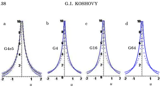
Fig. 2a shows the comparison of G0(u) calculation for 16: the solid line corresponds to the whole series; dots denote the sums of the first 4 and 5 terms. Graphical precision appears after the first 15 terms. Figs. 2b-2d compare calculations for G01(u) (firm line) and G0(u) for three values of :

4 (b), 16 (c), 64 (d).

(5)

138 G.I. KOSHOVY

Fig. 2 – Dependences of G0(u)

To determine the main characteristics of quasi-transverse waves we use the known approach based on the solution of the first kind singular IE with known right part of equation

1 3

0 1 1

( ) ( ( )) , 1, 1, , 3

m

in m

i m n

i

q t G x t dt x . (6)

Here index n indicates the strip with the unit potential (it also changes from 1 to 3m_{) and defines certain electrostatic problem: to find the} distri-bution of the surface charge density on the strips under the condition that all of them, except of the n-th one, have zero potential. In other words, we have 3m_{systems of IE with almost zero right part of equation:}

nm is the Kronecker symbol.

Comparing systems (5) and (6), we obtain the relationship between their solutions in the following form: 3

0i ( ) nm1 0n in( )

q t A q t . After integration of the last expression we find that 3

0i nm1 0n in

q A q , where q0i 11q0i ( )t dt. Then we use the correlations q0i 0q01i , which appear from (4) and connect solutions of the system (5) for > 1 and 1. Substituting into these solutions the corresponding sums, we obtain

3

0

0 1

1

( ) 0, 1,..., 3 .

m

n in in m

n

A q q i (7)

In the matrix form we have (Q v Q A0 1) 0 0. Thus, the problem of the determination of characteristics of quasi-transverse electromagnetic waves is transformed to the solution of the generalized problem of the eigenvalues of matrixes Q and Q1 formed by the elements qin at > 1 and 1. These matrixes are symmetric and positively determined, therefore the eigenvalues 0i are positive. They define the propagation constants of quasi-transverse electromagnetic waves by the approximation formulas hi 0ik. Correspon-dingly, the distribution of the surface current density on the strips is equal

to 3

0 1 1

( ) m _n _n( )

z n

j t A q t ,

G4e5 G4 G16 G64

u u u u

(6)

3

0 0 0 1

1

( ) ( ) ( )

m x

n n n

x

n

j x i A q t q t dt.

Here index indicates the strip where the mentioned function is considered. The possibility of taking into account the transverse component of the sur-face current density on the strips (it already depends on the frequency) is the significant difference of the given approach from the static one or T-approximation [11]. As a result of this possibility, in zero T-approximation another component of the surface current density is determined by the dis-tribution of the surface charge density in the system without dielectric base, i.e., 1. To coordinate the obtained expressions for the characteristics in the order of small frequency parameter , it is necessary to find the disper-sion corrections of the first order for h and jz(t).

4. INVESTIGATION OF THE DISPERSION

Dispersion corrections of the first order are determined by the equations similar to (5)

1 3

0

1 1

( ) [ ( ) ] , 1, 1, ,3 .

m

i m

i m i

q t G x t dt A x

Therefore using the applied algorithm we find the expressions for desired functions

3

1 ,1 1 ,1

1

( ) ( )

m

i n in

n

q t A q t .

In this case for the defined constants _A₁n_{we obtain that}

3 3

0 1

1 1 0 1

1 1

( )

m m

n in in n in

n n

A q q A q .

We multiply this equality by _A₀i_{, sum up and use the symmetry of matrixes}

Q, Q1 and equations (7). As a result, we obtain equality 1 (Q A1 0 A0) 0, from which we have ₁ 0 due to the positive determinacy of matrix Q1. Thus, dispersion corrections of the first order for h and jz(t) (in the case of simple eigenvalue 0i) are absent, and all expressions obtained in zero appro-ximation have an inaccuracy of the order of O( 2_ln – 1_{). To improve them it} is also necessary to consider the following approximation.

Dispersion corrections of the second order are determined by the equations 1

3

0 2

2 2

1 1

( ) ( ( )) ( ), 1, 1, ,3 .

m

i m

i m m

i

q t G x t dt A F x x (8)

Here

1

3 1 2

2( ) 2( ) 1 1 0( ) 2 ( ) , 2( ) 0 0 0( 0)2 m

i

m i

F u u q t G u t dt u B u A u ,

1 3

21( ) 2( ) 1 1[ 01( ) 21( ) 0 ( ) (0 )] m

i i

m m

i

(7)

140 G.I. KOSHOVY

G2(u), G21(u), P0(u) are the corresponding expansion coefficients of the kernels of IE system (2) in the small frequency parameter

0 2 0

2 ₂ 1 ₂ 0 2

0

2 1 2 1

( ) 2 ln ( , ) 4 ( ) ( , ),

1

G u i u i u

1 ₂ ₂ ₂

0

cos 1

( , ) ,

( cth 1) ( )

wu dw

i u

w w w w

2 ₂ ₂

0

sh 2 2 cos

( , ) ;

2 (ch 2 1) ( cth 1)

w w wu dw

i u

w w w w

21 0 1 0 2

0

2 1

( ) 2( 1) ln (1, ) 4( ) (1, ),

2 1

G u i u i u

0

2 0

1 2 ln

( ) 4(1 ) ln 4

1

cos 1

4( 1) .

( cth 1)(cth 1) ( )(1 )

P u

wu dw

w w w w w w

In the right part of equations (8) we have unknown terms A₂, which can be extracted from unknown functions q2i ( )t using solutions (6) in such a way as it was done in zero approximation

3

2 2 2

1

( ) ( ) ( )

m

i n in i

n

q t A q t p t .

New unknown functions p2i ( )t satisfy equation (8) without unknown A2 in the right part. To determine the dispersion correction of the second order ₂ we will use the corresponding correlation q2i 2q01i 0q21i following from (4). It can be represented in another form:

3 3

0 2 0

2 1 0 1 21 2

1 1

( )

m m

n in in n in i i

n n

A q q A q p p .

Multiply these equation by A0i, sum up and use (7). As a result, we find

3 3 3

2 0 0 1 0 0 21 2

1 1 1

( ) 0

m m m

i n in i i i

i n i

A A q A p p .

Expression for the dispersion correction of the second order can be easily obtained from the last equation due to the positive determinacy of matrix Q1

3

0

0 2 21

1 2

1 0 0

( )

m

i i i

i

A p p

Q A A . (9)

(8)

1 3

0 2

2 1 1

( ) ( ( )) ( ), 1, 1, , 3 .

m

i m

i m m

i

p t G x t dt F x x

Indeed, if multiply this equality by q0 ( )x , integrate, sum up and use the fact that function G0(u) is paired and equations (5), we obtain

1

3 3

2

0 2 0

1 1 1

( ) ( )

m m

i i

m i

A p q x F x dx.

Thus, numerator in (9) is completely determined by zero approximation and the corresponding expansion coefficients of the kernels of IE system (2)

1

3 3

0 2 0 21

0 2 21 0 01

1 1 1

( ) [ ( ) ( ) ( ) ( )]

m m

i i i

m m

i

A p p q x F x q x F x dx.

As a result, the expression 2 3

0[1 2 2 ]0 ( )

h k is obtained, and taking

it into account we can calculate the propagation constant of quasi-trans-verse electromagnetic waves.

5. CONCLUSIONS

The problem of electromagnetic wave propagation in the prefractal MSL system using the Raleigh method is investigated. This method separates the basic types of quasi-transverse electromagnetic waves. Transformation and simplification of the first kind singular integral equations used for the determination of the wave characteristics are performed. At first, zero or electrostatic approximation is studied in detail. Transformation of the kernel defined by the integral to the sum of the geometric progression is carried out as well as the numerical calculations. Frequency dependence and the possibility of taking into account the transverse component of the surface current density on the strips are manifested even in zero approximation. Furthermore the dispersion corrections of the propagation constants of quasi-transverse waves are considered. It is proved that the first order cor-rections with respect to the small frequency parameter for h and jz(t) (for the case of simple eigenvalue of the generalized problem of eigenvalues of (7)) are absent. Dispersion corrections of the propagation constants, which are of the order of O( 2_ln –1_{) and O(} 2_{) and which can be determined} with-out solving the IE (8) using zero approximation and known right part of (8), are obtained. We have to note about the possibility of application of the mentioned algorithm for the determination of the arbitrary order dispersion corrections relative to the frequency parameter .

REFERENCES

1. H. Henle, A. Mower, K. Vestpfall, Teoriya fifraktsii (M.: Mir: 1964).

2. E.I. Nefedov, A.T. Fialkovskiy, Poloskovye linii peredachi (M.: Nauka: 1980). 3. G.I. Koshovy, V.G. Sologub, Prepr./AN USSR. In-t radiofiziki i elektron. No322,

39 (1986).

4. A.G. Koshovy, G.I. Koshovy, Telecommun. Radio Eng.68, 1305 (2009).

5. G.I. Koshovy, Radiotekhnika155, 282 (2008).

(9)

142 G.I. KOSHOVY

8. V.F. Kravchenko, M.A. Basarab, Tech Phys. Lett. 29, 1055 (2003). 9. S.V. Krupenin, J. Commun. Technol. El.51, 526 (2006).

10.B. Mandelbrot, Fraktal’naya geometriya prirody (M.: Institut komp’yuternyh issledovanij: 2002).

11.Spravochnik po raschetu i konstruirovaniyu SVCh poloskovyh ustroistv (Red.