www.ocean-sci.net/3/485/2007/
© Author(s) 2007. This work is licensed under a Creative Commons License.
Ocean Science
Comparing the steric height in the Northern Atlantic with satellite
altimetry
V. O. Ivchenko1, S. D. Danilov1, D. V. Sidorenko1, J. Schr¨oter1, M. Wenzel1, and D. L. Aleynik2
1Alfred Wegener Institute for Polar and Marine Research, Bremerhaven, Germany 2The University of Plymouth, Plymouth, UK
Received: 23 April 2007 – Published in Ocean Sci. Discuss.: 16 May 2007
Revised: 12 October 2007 – Accepted: 15 November 2007 – Published: 28 November 2007
Abstract. Anomalies of dynamic height derived from an analysis of Argo profiling buoys data are analysed to assess the relative roles of contributions from temperature and salin-ity over the North Atlantic for the period of 1999–2004. They are compared with dynamic topography anomalies based on TOPEX/Poseidon and Jason altimetry. It is shown that the halosteric contribution to the anomalies of dynamic height is comparable in magnitude to the thermosteric one over the period analyzed. Taking both salinity and temperature into account improves the agreement between zonally aver-aged trends in the satellite dynamic topography and dynamic height increasing the correlation between them to 0.73 from 0.63 when only temperature variability is taken into account. The implication of this result is that the salinity contribution cannot be neglected in the North Atlantic and that one cannot rely on estimating the thermosteric part by anomalies in the sea surface dynamic topography derived from the satellite al-timetry.
1 Introduction
Whether the ocean is warming or cooling is an important question both in physical oceanography and for monitoring climate change. Temperature anomalies in the ocean lead to changes in the steric height and thus contribute to sea surface height (SSH) anomalies which can also be observed from satellites. This suggests using satellite altimetry to improve estimates of heat content tendencies (Willis et al., 2004) still suffering from sparsity of the in-situ data.
However, the variability of the SSH can be caused by dif-ferent oceanic processes. In addition to steric height changes it is affected by redistribution of the water masses in the ocean or barotropic component of sea-surface height (Willis Correspondence to:V. O. Ivchenko
et al., 2003, 2004), or direct changes in the total ocean mass (sea level rise). The steric height variability itself depends not only on temperature but also on salinity anomalies. Thus the temperature signal in the SSH anomalies is masked by other influences.
Many authors suggest that the temperature anomalies in the upper few hundred meters is the leading factor determin-ing both steric height and SSH anomalies and disregard the influence of the salinity variation. Such analyses are made either for the global ocean (Willis et al., 2003) or for its particular regions (White and Tai, 1995). Note, that even if the thermosteric effect dominates over the halosteric one in the globally averaged steric height, this is not necessarily true locally. Antonov et al. (2002) point out that the salin-ity effects are crucially important in some regions, includ-ing the subpolar North Atlantic. However, the haline effects play a minor role for the spatially averaged steric height be-tween 50◦S and 65◦N for the 1957–1994 period. Sato et al. (2000) demonstrate importance of salinity for the heat storage estimation from TOPEX/Poseidon in the in situ data for three points at low latitudes in the Pacific and Atlantic. Gilson et al. (1998) demonstrate that including salinity mea-surements significantly reduces errors in specific volume and steric height in the North Pacific. Maes (1998) discusses different possible mechanisms in tropics, subtropics and the Southern Ocean by which the salinity variations may gener-ate a signal in sea level.
Summing up, the following problems need to be resolved:
– What is the relative importance of variability of salin-ity and temperature in their contribution to the steric height?
of the North Atlantic for the 10◦boxes for the 1999–2005.
– In which regions can one expect increased halosteric contributions?
The availability of the Argo floats data suggests a unique possibility to address these questions which is the main goal of this paper. Our analysis below is limited to the North At-lantic basin and mainly concentrated on the first problem. We should add the caveat that period of five years is insufficient for an accurate computation of the ocean trends.
We describe the data used and their preparation in Sect. 2. Sections 3–5 present our main results, discussion and con-clusion, respectively.
2 Data and method
Temperature and salinity profiles from the Argo project were used for calculations of steric height. The analysis is limited to the North Atlantic basin between 10◦N and 70◦N and to the period between January 1999 to December 2004. The data were obtained from the official Argo web-site. They comprise 31 949 temperature profiles and 19 108 salinity pro-files. Quality control flags provided by the originators were used to eliminate inappropriate profiles, which led to some reduction of the data set. The data set was further reduced by eliminating profiles that differ by more than 4 standard deviations from the monthly averaged values in 10 by 10 de-gree boxes. In the February 2007 the Argo users were in-formed that profiles from SOLO floats with FSI CTD (Argo Program WHOI) may have incorrect pressure values. For this reason all observations by this type of instrument were removed from our data set. The number of profiles decreases to 22 529 and 16 088 for the temperature and salinity data, respectively.
The mean coverage of the Northern Atlantic with floats is shown in Fig. 1a. It is not uniform with a maximum over the central North Atlantic and minima along the coast. The coastal regions correspond to about 10 profiles in a 10 by 10 degree box per month of observations. It is worth men-tioning that there is considerable improvement in coverage of the North Atlantic from 1999 to 2004 almost everywhere, ex-cept for the western part of the zonal belt between 20◦N and
which is optimal in the least squares sense. The covariance of the data is assumed to be Gaussian with the correlation lengthL=350 km everywhere within the domain. This value is more than twice the value used by Lavender et al. (2005), but is justified by the data distribution within the domain used here.
The altimetry data set used for comparison is based on the TOPEX/Poseidon/Jason missions and was provided to us by S. Esselborn (GFZ Potsdam). It covers a period from 1993 to May 2005. Both Argo and altimetry monthly mean anoma-lies were interpolated to 1 by 1 degree grid.
The steric height is defined as an integral between the sur-face and some depthD(or pressure) of the specific volume anomaly δ computed with respect to a temperature of 0◦C and a salinity of 35 psu (Gill, 1982). A depth of 1000 m was used for the most of the presented results (see Sect. 4). The monthly anomalies of steric height (ASH) were computed with respect to their mean annual cycle over January 1999– December 2004 while the mean annual cycle over a longer period of time (1993–December 2004) was used to compute anomalies of satellite altimetry (ASA). Due to difference in averaging periods there is offset of the ASA with respect to ASH. It is computed as the difference between mean values of the ASH and ASA over the last six years and compensated for the comparison of the anomalies.
The error estimates for trendsσα are computed asσα =
σf ld
σ[1...n]
· 1−r 2
(n−1)1/2, whereσf ld is the standard deviation of
a field (sea surface satellite altimetry or steric height) forn
years,σ[1...n]is the square root of the variance of the set of years from 1 ton, andris the correlation coefficient between the regression and the variability of the field.
3 Results
3.1 Steric height vs. altimetry
Fig. 2.The ASH (red) and ASA (blue) anomalies averaged over the Northern Atlantic.(a)– full anomalies;(b)– the seasonal cycle of the ASH and ASA; the averaging time is between 1999 and 2005 and between 1993 and 2005 for the ASH and ASA, respectively;(c)
– The anomalies after removing the seasonal cycle. The green curve shows ASH for the experiment with the half of the data excluded. The ASA curve is shifted down by the difference between the mean over last six years and the total mean. The units are in m.
thermocline this difference should be attributed mostly to non-steric contributions into the ASA.
Removing the seasonal cycle of both data sets leaves anomalies of smaller amplitude which are considered further. Panel C of Fig. 2 shows the basin averaged ASH (red) and ASA (blue) for both data sets. They are generally consistent and show variability of similar amplitude within individual years. The trend for the ASA is 2.58 mm/year and larger than the trend of the ASH, which is 1.44 mm/year with stan-dard errors of 0.38 mm/year and 0.37 mm/year for the ASA and ASH, respectively. The trends are computed over last six years.
Annually averaged fields of the ASH and ASA were com-puted to exclude the influence of the seasonal cycle and vari-ability on short time scales. The differences in horizontal distributions between two consecutive years (not reproduced here) have much in common for ASH and ASA in spite of their inherently different patchiness.
In order to simultaneously characterize the entire period of observation we computed linear regression for five annual mean values at every grid point for ASH and ASA (i.e. 2000– 2004; 1999 was excluded because salinity measurements are less dense). Figure 3 depicts the pattern of trend found for the satellite data (Fig. 3a) and steric height (Fig. 3b). The values of the trend of the surface height and the steric height are larger than the values of the errors shown in Fig. 3c, d.
Fig. 3. The trends of the altimetry and steric height anomalies for the period 2000–2004. Panels(a), (b),(e)and (f)correspond to trends in satellite altimetry, full steric height and the thermosteric and halosteric contributions, respectively. Panels (c) and (d) present trend uncertainties for ASA and ASH respectively.
Once again, there is a reasonable similarity between the trend patterns. Predominantly positive trends occur in the south-ern, northern and mid western domains of the basin in both fields. Mostly negative values are in the mid North Atlantic and subpolar gyre in both fields. However, contrary to the negative trend of the ASH in the south-east corner of the basin the trend in the ASA is positive here with exception of small area in the vicinity of Africa. A similar difference is found for the Labrador Sea where we see a negative trend in the steric height but a positive trend in the satellite altime-try. A possible reason for such a difference in behavior can be a bias due to insufficient amount of the Argo data in these regions (see Fig. 1).
3.2 Roles of temperature and salinity anomalies
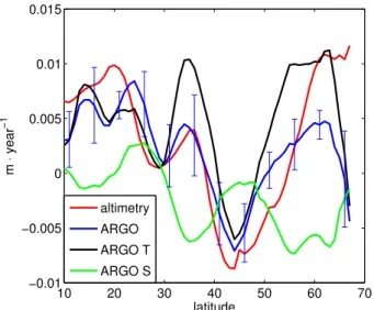
10 20 30 40 50 60 70 −0.01
−0.005
latitude altimetry
ARGO ARGO T ARGO S
Fig. 4. Zonally averaged trends between 2000 and 2004 for the satellite altimetry (red), full steric height (blue), and thermosteric (black; salinity is climatological)) and halosteric (green; tempera-ture is climatological)) heights. The vertical bars represent uncer-tainties.
temperature contributions into ASH are of similar magnitude (several centimeters) although the pattern of thermal contri-bution in the ASH is closer to ASA. In many places, the salin-ity anomalies act against the temperature anomalies. This fact is best seen in patterns of trend due to thermal expansion and saline contraction shown in Fig. 3e and f respectively.
The main contribution to the profound positive signal in the northern and southern domains comes from temperature anomalies. Similarly, a predominantly negative trend in the ASH above the center of the North Atlantic Ridge comes from the temperature. However, the importance of the contri-bution of salinity anomaly is clearly seen over the eastern do-mains and close to the U.S. coast starting at 30◦N. A strong positive trend of the ASH near the African coast (which is not observed in the satellite altimetry trend) is partly compen-sated by the strong negative ASH coming from the halosteric part.
In order to estimate a typical value of local trends we computed their rms values. The rms value of the trend of the ASA is higher than that of the steric height (8.5 and 7.7 mm/year, respectively). The rms value of the steric height lies between the corresponding values of the “temper-ature only” and “salinity only” experiments which are 9.6 and 5.6 mm/year, respectively. Thus the impact of salinity anomalies on the steric height is to partly compensate the temperature influence.
There is a strong similarity between the zonally averaged trends of ASH and ASA as demonstrated by Fig. 4. The correlation between the corresponding curves is relatively high and reaches 0.73. The correlation between thermosteric anomalies and ASA drops down to 0.63 while it becomes
ticorrelated changes in temperature and salinity. That is why our result is not unexpected.
To illustrate this issue we computed yearly averaged anomalies of the depth of neutral density surface γ=27.5 (ADNDS). The differences in ADNDS between consecutive years are mainly due to the temperature variability for the first several years (2000–1999 and 2001–2000). This can be partly a consequence of inadequate coverage of salinity data for the first two years. In the following years (2002–2001 and 2003–2002), the contribution from the “salinity only” is even stronger than the contribution from the “temperature only”.
The change of depth of the neutral surface γ=27.5 be-tween 2004 and 2003 in Fig. 5 demonstrates the importance of both temperature and salinity contributions in forming this change. A large negative displacement of the neutral sur-face in the eastern southern and middle parts is apparently associated with salinity anomalies. Over other places like the western middle part and the northern part the positive values are mainly related to the temperature field. The rms displacement due to both temperature and salinity anoma-lies is 16.9 m. Thermally induced rms displacement is larger (20.2 m), and the rms displacement due to “salinity only” is 19.6 m.
4 Discussion
Fig. 5.The variation of the depth of the neutral surface of 27.5 between 2004 and 2003 due to both temperature and salinity anomalies (left), temperature only (middle) and salinity only (right).
similar to the full data set (Fig. 2, lower panel) with the cor-relation coefficient of 0.84 (the data were filtered with a 5 point low pass filter). The trend of the ASH decreases from 1.44 mm/year (error of 0.37 mm/year) to 0.84 mm/year (error of 0.42 mm/year) when data coverage is reduced from full to 50%, respectively.
The choice of a reference depthDis not a trivial problem. It should be deep enough so that the steric height is not sen-sitive to its further increase (this surface does not necessarily exist). Our experiments show that the depth of 1000 m is a good first approach forDin the North Atlantic. We checked that computing ASH referenced to 1500 m does not change conclusions drawn here and opted for a shallower depth of 1000 m to have a better data coverage.
The total steric height anomalyha can be split into two contributions,ha=ha1+ha2, one from the water column
be-tween the surface and depth of seasonal thermoclinehs(ha1)
and the other betweenhs andD(ha2). The total anomaly is
dominated byha1over the seasonal cycle. The seasonal cycle
in mid latitudes is much more profound in temperature than in salinity field. The changes of heat content in the seasonal thermocline are mainly a consequence of the net surface heat flux (Yan et al., 1995; Stammer, 1997). As a result changes of the steric height due to the seasonal thermocline can be calculated by using net surface heat flux. The deep partha2
becomes a major contribution on longer (interannual) time scales or if the seasonal cycle of steric height is removed and salinity anomaly can be an important contributor to this part. Usually the thermosteric and halosteric contributions to the steric height anticorrelate (see Fig. 4), i.e. partly com-pensate each other. This is not surprising, because the mo-tion below the seasonal thermocline occurs along isopycnals and the salinity of a moving water parcel must be higher if its temperature is higher to retain the same density.
5 Conclusions
The analysis above shows that both temperature and salin-ity determine the variabilsalin-ity of steric height in the North Atlantic over a 5-year period considered here. Considering only temperature variability leads to a basin averaged trend of 2.7 mm/year which is about of two-fold larger than the to-tal trend in the steric height. Although this value is closer to the trend in basin averaged altimeter anomalies this closeness is only superficial. There is indeed improvement in the agree-ment between trends after inclusion of salinity anomalies as is best seen in zonal averages (see Fig. 4). On the local scale, the contribution from temperature and salinity are of similar magnitude.
The positive temporal trend in the surface height (from satellite altimetry) is higher than the trend in steric height only. It implies that other contributions of non-steric nature also play an important role in the North Atlantic over time scales studied here.
Acknowledgements. We are grateful to S. Esselborn for providing
the altimeter data. VOI was supported by the UK NERC (RAPID program) whilst preparing the objective analysis of the Argo data.
Edited by: N. C. Wells
References
Antonov, J. I., Levitus, S., and Boyer, T. P.: Steric sea level vari-ations during 1957–1994: Importance of salinity. J. Geophys. Res., 107(C12), 8013, doi:10.1029/2001JC000964, 2002. Bretherton, F. P., Davis, R. E., and Fandry, C. B.: A technique for
objective analysis and design of oceanographic experiments ap-plied to MODE-73, Deep-Sea Res., 23, 559–582, 1976. Gandin, L. S.: Objective analysis of meteorological fields.
Leningrad, Gidrometeoizdat, 287 pp. (in Russian), English trans-lation No. 1373 by Israel Program for Scientific Transtrans-lations, (1965), 242 pp., 1963
in the ocean, Geophys. Res. Lett., 25(19), 3551–3554, 1998.
Stammer, D.: Steric and wind-induced changes in
TOPEX/POSEIDON large-scale sea surface topography observations, J. Geophys. Res., 102, 9, 20 987–21 009, 1997. Stephens, C., Antonov, J. I., Boyer, T. P., Conkright, M. E.,
Lo-carnini, R., and O′Brien, T. D.: World Ocean Atlas 2001, 1: Tem-perature (CD-ROM), eds. by S. Levitus, NOAA Atlas NESDIS 49, U.S. Govt. Printing Office, Washington, D. C., 2002.