Is land surface temperature
an earthquake precursor?
Ardit Sulçe
Submitted in partial fulfilment of the requirements for the degree of
Master of Science in Geospatial Technologies
ii
Dissertation supervised by:
Prof. Edzer Pebesma, Ph.D.
Institute for Geoinformatics
University of Muenster
Muenster, Gemany
Dissertation co-supervised by:
Prof. Mario Caetano, Ph.D.
Instituto Superior de Estatística e Gestão de Informação
Universidade Nova de Lisboa
Lisbon, Portugal
Prof. Filiberto Pla, Ph.D
Departamento de Lenguajes y Sistemas Informatícos
Universitat Jaume I
Castellon, Spain
iii
Declaration of originality
iv
Acknowledgment
“Whatever the cost of our libraries, the price is cheap compared to that of an ignorant nation.” - Walter Cronkite.
Following the quote above, I would like to start by thanking the financial supporter of this program, European Commission, without whom, not only me, but thousands of other students would not have been able to gain the aspired precious knowledge and to contribute their wisdom to the betterment of humanity.
I would like to express my gratitude to my thesis research supervisors, Prof. Edzer Pebesma, Prof. Mario Caetano and Prof. Filiberto Pla for supervising my research by giving valuable feedback that helped me view the ideas, problems and solutions in different perspectives.
I would like to thank my fellow students for sharing their knowledge and their experiences and for being part of this exciting learning experience in such a rich and stimulating educational program.
v
Abstract
This study aims to investigate and explain the land surface temperature variations before and after the earthquake of August 11, 2012 that struck Iran, by making critical considerations of weather factors. This goal underlies two main objectives. The first objective was to detect land surface temperature anomalies over time in respect to the day of the earthquake, and over space relative to the location of the earthquake epicentre. The other main objective was to determine whether the detected anomalies originated from the weather, or the earthquake. To meet these objectives, observations of remote sensing land surface temperature, near-ground air temperature and air temperature of multiple atmospheric levels were used. All the datasets were daily night-time observations extending to a period of five years, repeatedly from July 11, to August 31.
All the observations of the three datasets were visualized in space and time to seek anomalous temperature patterns. The results showed several prominent land surface temperature increases over the 5-year period, but none of them fell out a few days before the earthquake. The most enduring land surface temperature increase occurred two days after the earthquake. In contrast to the land surface temperature, air temperature exhibited the sharpest anomalies of the entire period a few days before the earthquake. Both the air and the land surface temperature increased periodically few times within the 5-year period. The high temperature patterns that were detected in the near-ground air also matched in time with the patterns found in the temperature of multiple atmospheric levels.
vi
Contents
Declaration of originality ... iii
Acknowledgment ...iv
Abstract ... v
Index of figures... viii
Keywords ... ix
Acronyms ... ix
1. Introduction ... 1
1.1. Background ... 1
1.2. Research questions ... 2
1.3. Theoretical background ... 3
1.3.1. The mechanism of thermal earthquake precursors... 3
1.3.2. Similar studies ... 3
1.3.3. Heat exchange between land surface and air ... 5
2. Data and quality assurance ... 5
2.1. Data ... 5
2.1.1. Land surface temperature satellite images ... 5
2.1.2. Near-ground air temperature observations ... 7
2.1.3. Atmospheric air temperature observations ... 7
2.2. Quality assurance... 7
2.2.1. Quality assurance of the land surface temperature satellite images ... 7
2.2.2. Quality assurance of the near-ground air temperature observations ... 8
2.2.3. Quality assurance of the atmospheric air temperature observations ... 8
3. Methodology ... 8
3.1. Pre-processing of satellite images ... 8
3.2. Land surface temperature normalization ... 9
3.3. Approach 1: detecting land surface temperature changes in space and time ... 10
3.3.1. (a) Plotting land surface temperature in a time-temperature graph... 10
3.3.2. (b) Plotting land surface temperature in a time-space-temperature graph ... 11
3.4. Approach 2: detecting anomalous differences between land surface and near-ground air temperature ... 13
3.5. Approach 3: detecting temperature changes in the vertical atmospheric column above the earthquake epicentre ... 15
vii
4.1. Land surface temperature changes in space and time ... 15
4.2. Anomalous temperature differences between land surface and near-ground air ... 21
4.3. Temperature changes in the vertical atmospheric column above the earthquake epicentre. 21 4.4. Discussion ... 25
5. Conclusions ... 27
6. Recommendations ... 28
viii
Index of figures
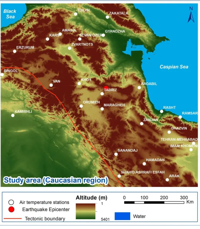
Figure 1: Study area comprising an approximately 1000 x 1000 km region; distribution of air temperature stations ... 2
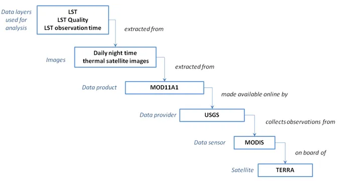
Figure 2: Diagrams of LST satellite image data acquisition ... 6
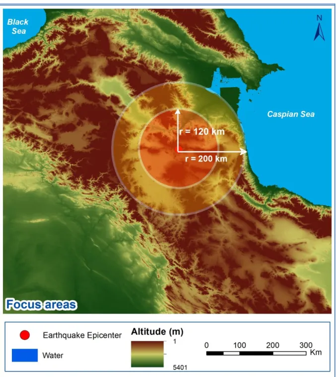
Figure 3: The three areas for which the LST was calculated: (a) the area extending 120 km from the epicentre, (b) the area extending 200 km from the epicenter and (c) the entire area... 11
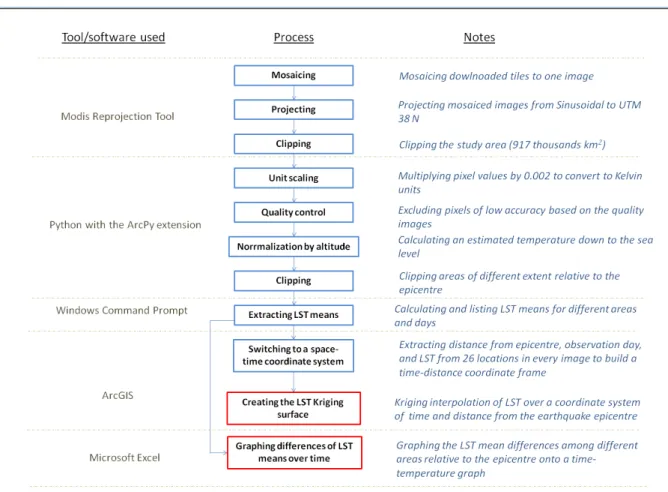
Figure 4: Methodology diagram of "Approach 1” listing major processes starting from the input data
to the two final graphs ... 12
Figure 5: Differences in LSTs of areas with different extents relative to the earthquake epicentre. Positive values indicate higher land surface temperature of the areas close to the earthquake compared to the entire area. No anomalies exist a few days before the earthquake... 19
Figure 6: LST Kriging surface in a coordinate frame of time horizontally, and epicentral distance vertically. Seasonal warm LST patterns repeating every year can be observed over time in the area extending up to 200 km from the epicentre. The surface was created using daily night time remote sensing LST observations. ... 20
Figure 7: Kriging surface of differences in temperature between land surface and near-ground air in a coordinate frame of time horizontally, and epicentral distance vertically. Land surface temperature exhibits the lowest values compared to air temperature ... 21
Figure 8: Daily air temperature measured at 3 different atmospheric levels. Temperature exhibits a normal behaviour in the days before the earthquake. All the three levels show similar trends. The graph was created using weather balloon radiosonde night time daily temperature observations. .. 23
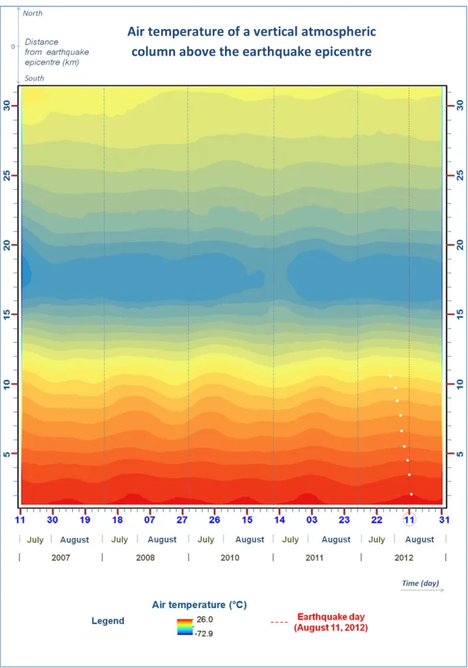
Figure 9: Air temperature of the vertical atmospheric column. The white dots indicate that the warm pattern originated earlier in the high atmosphere to propagate later down to the lower layers. The graph was created using weather balloon radiosonde night-time daily temperature observations. . 24
ix
Keywords
Air temperature
Land surface temperature
LST
Thermal remote sensing
Temperature anomalies
Earthquake prediction
Acronyms
DEM – Digital Elevation Model
IGRA – Integrated Global Radiosonde Archive
ISD – Integrated Surface Database
LST – Land Surface Temperature
MODIS – Moderate Resolution Imaging Spectrometer
MOD11A1 – MOD_L2 projected to sinusoidal projection
MOD11_L2 – Level 2 MODIS LST product
NCDC – National Climatic Data Center
NOAA – National Oceanic and Atmospheric Administration
QC – Quality Check
1
1.
Introduction
1.1.
Background
Earthquake prediction has for decades been, and still is a challenging target for the scientific community. A wide range of precursor phenomena ranging from abnormal animal behaviours to temperature anomalies are claimed to have been spotted before big earthquake events (Cicerone et al., 2009). One of these precursors is believed to be land surface temperature (LST). Detecting LST anomalies as earthquake precursor is also the focus of this study. The big earthquake of August 11, 2012 in the northwest of Iran is the event in focus. The earthquake had a magnitude of 6.5 and resulted in a death toll of nearly 300 people (Torbati, 2012).
A number of similar studies aiming to detect LST anomalies have been done. The majority of them has claimed LST increase from 2 to 4 ˚C occurring 2 to 10 days prior to big earthquakes. The focus of the analyses of these studies has been the comparison of the LST for the period preceding the earthquake with the average LST of the same season, but for other years that experienced no earthquake in the area of interest.
In contrast to previous studies where LST has been a stand-alone analyzed variable, in this study, air temperature data were also incorporated into the analyses with the goal to understand the weather effect on the expected LST variations. In other words, the objective of this study is not merely detecting LST anomalies a few days before the earthquake, but also explaining their origin.
To accomplish what was just stated, three different datasets were used: (a) LST satellite images, (b) near-ground air temperature observations, and (c) air temperature observations of multiple atmospheric levels. All these data were daily observations taken at night-time between 9 PM and 12 PM. The reason behind analyzing night-time observations is because the sun irradiation effect is minimal during that time (Laughton, 2010). Therefore, there is much less possibility that the anomalies will be masked by other factors. Each of the datasets was used in three different approaches to detect and understand the possible land surface temperature anomalies. The period of the observation extends from 2008 to 2012 repeatedly for the period from July 11 to August 31.
2
Figure 1: Study area comprising an approximately 1000 x 1000 km region; distribution of air temperature stations
1.2.
Research questions
The research questions listed below were raised on the basis of this research:
1. Are there land surface temperature anomalies in the few days before the earthquake of August 11, 2012 in the area extending within a 200 km radius from the epicentre? Are these anomalies sharper in the area within 120 km from the epicentre?
3
3. Is the temperature increase, if any, a localized pattern in the low atmosphere or is it a seasonal pattern with a similar vertical extent as in other periods?
4. Do all three research approaches lead to the same conclusion and If not, why?
1.3.
Theoretical background
1.3.1.
The mechanism of thermal earthquake precursors
Several phenomena are believed to trigger the increase of land surface temperature before earthquakes strike. However, these phenomena are still vaguely understood and not widely accepted by the scientific community.
An earthquake phenomenon itself is generated from a few to dozens of kilometres deep underground. Rock pressure builds due to the continuous movements of the tectonic plates and causes rock ruptures. The sudden movement will then send seismic waves up to the earth’s surface. This process is associated with a significant energy release (Scholz, 2002).
Before earthquakes occur, rock pressure is thought to be the very origin that triggers temperature increases on the land surface. The stress accumulation is believed to emit thermal infrared waves which themselves are thought to increase the thermal activity (Ouzounov and Freund, 2004).
Creation of micro-pores in the earth’s crust because of pressure built is another proposed phenomenon. This is believed to allow gases to travel up to the near surface causing temperature increase (Saraf et al., 2009).
Radon, a radioactive element found both in soil and air is also thought to be an important earthquake precursor. Studies claim that radon is ionized before earthquakes strike. Its ionization leads to increased humidity which causes the temperature to increase (Pulinets et al., 2006). While some studies investigate the thermal effect of this phenomenon, other studies (Singh et al., 1999) have done more direct research on radon as an earthquake precursor by analyzing its amounts in ground waters.
Well water levels have also been a research subject for a long time in this field. Their increase is believed to be an earthquake precursor (Igarashi and Wakita, 1991). Besides this direct relation, there is also an indirect one that has to do with land surface temperature. Supposedly, the well water rise causes temperature to propagate through soil up to the land surface (Ouzounov et al., 2006).
Even though the list of the phenomena related to the thermal precursors is rich, their mechanism is poorly understood and their acceptance by the scientific community is still humble.
1.3.2.
Similar studies
4
Weather seems to be a factor that has not been taken into consideration throughout the studies done so far in efforts of detecting LST anomalies. This omission is not because weather is a factor that does not affect LST, but because it is difficult to predict and understand its behaviour. Some studies have also analyzed air temperature, but no studies appear to have studied both LST and air temperature in order to count for their interaction.
Mainly, the detection methodologies of thermal precursors have been designed to compare the temperature of the days preceding the earthquake with the temperature of the same season, but in another year where there was no earthquake. These LST time series analyses have been performed for area surrounding the earthquake epicentre. In Ouzonov and Freund (2004), the LST was compared with the mean of two other years. Robust satellite technique has also been a widely applied technique, not only for detecting thermal precursors (Lisi et al., 2010) but even broader in monitoring seismic hazards (Tramutoli et al., 2001), (Aliano et al., 2008).
Evaluations of different methods of detecting thermal precursors have also been performed concluding that all the methods were able to reveal anomalies, but with no certainty on their relation with earthquakes (Okyay, 2012).
Along with the varying conclusions about whether the thermal precursors exist or not, their quantification has also varied. Different studies have claimed different occurrence times of the LST anomalies with a wide range from 2 to 24 days before the earthquake, an indicator that may cast doubts on the real source of these precursors. In Ouzunov (2006), the LST anomalies were found to occur 4 to 14 days before the earthquake. In Tronin et al. (2002), the anomalies were claimed to occur 6 to 4 days before the event.
Similarly to the diversity on how many days in advance earthquake thermal precursors emerge, their spatial extent has also been dubbed with a wide range. Some studies have found that the temperature anomalous patterns had a small extent of few kilometres away from the epicentre while some others have concluded ranges of hundred kilometres. In Tronin et al. (2002) for instance, the LST anomalous patterns had a spatial extent of 700 x 50 km, which is an area of an unsymmetrical shape differing from what the other studies have concluded.
The temperature magnitude of the detected anomalies has also had a wide range, from 2 to 12 ˚C. In Ouzounov et al. (2006) and Saraf et al. (2009), many earthquakes were studied and the variation of temperature was in the interval of 2 – 4 ˚C. There are also other cases when higher amplitudes ranging from 5 to 12 ˚C have been found.
Besides studies that recognized the existence of LST anomalies before earthquake events, there are other ones that have not found any relation between earthquakes and thermal signals. There are also cases where precursors have been spotted, but cautious interpretations have been made, concluding that the anomalies found cannot be related with the earthquake as the increased thermal activity was also present in other periods of time (Okyay, 2012).
Criticism has also followed not only the idea of detecting thermal precursors, but other earthquake prediction efforts as well (Geller, 2007). In some cases such as in Geller et al. (1997) the speculations have reached the point to make definite statements that earthquakes cannot be predicted.
5
psychological caution seems to not have been taken into consideration when interpreting the results in the majority of the previous studies that have analyzed temperature as an earthquake precursor.
1.3.3.
Heat exchange between land surface and air
In order to count for the weather behaviour, besides LST analyses, the scope of this study extended to air temperature analyses of both near-ground and upper atmosphere reaching 30 km above ground level. Starting from just above the ground and going up to higher atmospheric levels, different layers having different properties are met. The very first layer of air extends 1-3 cm above the ground. It is considered a separate layer due to its tight relations with the land surface. This layer is heated directly by the land surface and it has a very inefficient heat exchange with air mass above. The differences between this shallow layer and the air above can reach up to 15 ˚C (Hackworth, 2004). It therefore acts as an isolating layer between the land and the air mass above it. Looking at the differences between LST and air temperature would therefore reveal important clues if the land was to be heated by any source other than weather.
On a broader scale, another first layer is defined by meteorology. This layer is named “boundary atmospheric layer”. It is a layer extending from a few hundred meters above the poles to 1 km above the equator. Its definition identifies it as a layer where the effects of the surface such as friction, heating and cooling are felt directly on time scales less than one day (Garratt, 1994). Radon, an element that is thought to be related to earthquake precursors is found in considerable amounts in this region compared to other layers of the atmosphere (Porstendörfer et al., 1991).
As altitude increases, the temperature decreases linearly. This is known as the lapse rate and has a value of 6.5 ˚C / km (Minder et al., 2010). This relation allows for estimation and interpolation of temperature. These interpolated surfaces then can be used to visualize temperature and possible anomalies in different levels of the atmosphere.
2.
Data and quality assurance
The data used in this study were acquired from USGS and NOAA. Specifically, remote sensing observations such as LST and DEM were provided by USGS, while the air temperature observations from ground stations and weather balloon radiosondes were provided by NOAA. In both cases the data were downloaded online from the respective websites. In more details the data are described in section 2.1 while the quality assurance process is described in section 2.2.
2.1.
Data
2.1.1.
Land surface temperature satellite images
6
itself is the result of a generalized split window algorithm used to retrieve the land surface temperature (Wan, 2006).
This split window algorithm corrects for atmospheric effects based on the differential absorption in adjacent infrared bands (Wan and Dozier, 1996). In the case of land surface temperature, these adjacent bands are bands 31 and 32. The thermal information is collected by the MODIS sensors via these two bands. These two sensor channels correspond to a bandwidth of 10.780 - 11.280 and 11.770 - 12.270 µm respectively (Maccherone). These channels are also referred as atmospheric windows as they can receive specific wavelength radiation from earth with minimum loss as the signal travels through the atmosphere. These signals are then registered in grid format and converted to digital numbers to be distributed in the form of images. Along with the land surface temperature data, the image products also contain other information such as accuracy indicators, time and angle of observation on a pixel basis and other relevant information. Part of this information comes in the form of image layers and other metadata in textual form.
The MOD11A1 product image layers used in this research are (a) night-time LST, (b) night-time LST quality control and (c) night-view-time. The spatial resolution of the images is 1200 by 1200 pixels with a pixel dimension of 927 by 927 m. The LST accuracy varies at an average of ±1 K depending on emissivity, atmosphere content, sensor view angle, etc. The information about accuracy is given on a pixel basis (Wan, 2006). Accuracy issues are discussed in more depth in section 2.2.1.
260 daily LST images for July, 11-August, 31 repeatedly for the period 2008-2012 were used. The time of the observations varies from 9 PM to 10 PM and is consistent with the air and atmospheric observations datasets. These LST remote sensing observations were acquired from USGS (USGS, 2013).
7
2.1.2.
Near-ground air temperature observations
Daily night-time air temperature data of ground stations located 2 m above ground were used to secure the near-ground air temperature data used in the second method. The ground observations are made available by NOAA through ISD. ISD is a database containing weather observation data taken hourly by thousands of ground weather stations worldwide.
26 stations spread through the study area were found to have consistent data and therefore were used accordingly for the second method. The observations belong to the same period of time as in the case of LST satellite images, specifically from July 11, to August, 31 repeatedly for all the years within the period 2008-2012. The average of temperature observations taken between 9 PM and 23 PM was calculated to retrieve the air temperature of the same time of the night as in the case of LST satellite images. The near-ground air temperature was acquired by NOAA website (NOAA, 2013).
2.1.3.
Atmospheric air temperature observations
Daily night-time air temperature data of atmospheric layers were used for analyses in the third method. The observations are taken daily by radiosondes attached to weather balloons and made available by NOAA through IGRA archives.
The daily observations of a station located 35 km away from the earthquake epicentre were used to analyze the temperature of the atmosphere. The observations are taken every 1.5 km vertically starting from the ground and up to 30 km above it.
The observations used belong to the period from July 11 to August 31, repeatedly for the years 2007, 2009-2012. This is the same period as the LST and ground air temperature data with the difference that the data from 2007 were used instead of 2009 due to an incomplete dataset in the latter one. All the observations are taken starting at 12 AM until 1 AM every day as the weather balloon rises up to 30 km. The data were acquired from NCDC (NCDC, 2013).
2.2.
Quality assurance
Quality check was performed for all the data used in this study. All the temperature values were associated with quality flags, which are indices that describe the quality of the observations. More details on how the quality assurance was performed are given below for each dataset.
2.2.1.
Quality assurance of the land surface temperature satellite images
The LST image datasets have gone through two quality check phases described below:
The first phase has been performed by the data providers. In this process LST images have been validated with insitu measurements in more than 50 clear sky cases in the temperature range from
-10oC to 58oC (Wan, 2006).
8
land emissivity effects on the LST. The flags are associated with every LST image pixel value. Based on the quality check flags, pixels with emissivity error greater than 0.02 and LST error greater than ±2 K were excluded from the LST images.
2.2.2.
Quality assurance of the near-ground air temperature observations
The air temperature values that had passed all the quality checks according to the quality flags were used for the study. This filtering process found only a few erroneous values. 99.9 % of the data passed the requirements and therefore were used for the analysis.
2.2.3.
Quality assurance of the atmospheric air temperature observations
The temperature values of the radiosonde atmospheric observation were also associated with quality flags. According to the quality flags, values that fell within the "tier-1" climatological limits based on all days of the year and all times of the day at the station were used for the analysis. Nearly 50% of the values satisfied these quality requirements yet without affecting the homogeneity of the observations’ vertical intervals.
3.
Methodology
All three datasets, the LST, the near-ground air temperature and the atmospheric observations were pre-processed and formatted to be consistent for being used in the analyses. Additionally, the LST was normalized by altitude using a digital elevation model with a pixel size of 1x1 km - the same as the LST images.
The three research approaches are described after the pre-processing and normalization sections. The first approach aims to detect LST anomalies in space-time by generating two different graphs that represent LST in two different perspectives which complement each-other in terms of information conveyed. In the second approach, differences between air temperature and LST are plotted, again in a space-time coordinate frame that allows comparative interpretations between the two variables in both space and time. In the third approach, a vertical atmospheric column profile is generated in order to visualize and analyze the temperature patterns in a broader view. This atmospheric column of air temperature will be the base for determining if the LST and air temperature variations found in the two previous approaches were localized patterns or patterns that have a consistent behaviour with the upper layers of the atmosphere.
3.1.
Pre-processing of satellite images
As part of the pre-processing phase, the downloaded image tiles were mosaiced, projected to Universal Transversal Mercator projection, zone 38, North, and clipped to the study area. This was accomplished using MODIS Reprojection Tool.
9
approximately 500 km in terms of the distance from the epicentre, which is located approximately in the centre of the area. After the study area was well defined, the quality control process took place in order to exclude low quality pixels.
The units of the image values were scaled to be converted to Kelvin according to the scale coefficients given in the MODIS user product guide. Both quality control and unit scaling processes were performed using Python with the ArcPy extension.
3.2.
Land surface temperature normalization
Taking advantage of the high correlation between altitude and temperature, the LST images were normalized by terrain altitude. In every 1 km increase of altitude, the temperature decreases with 6.5 ᵒC (Minder et al., 2010). This normalization of LST was done for two reasons.
First, the normalization by altitude allows possible LST anomalous patterns to visually emerge in the satellite images as it balances out a great factor of the temperature change - altitude. The second and more important reason for normalizing the LST is related to the issue of missing pixel values. The lack of the pixel values is a phenomenon that primarily occurs due to cloud cover and therefore it is not selective –it might happen in different regions of different altitudes in different days. Due to this heterogeneity, during the LST comparative analyses, temperatures of different altitudes will have to be compared with each other. Therefore, the comparison process would not be correct as the temperature values would be altitude-dependent. In contrary, comparing temperatures of the same altitudes would give more accurate results.
To conclude the idea, a digital elevation model of the study area was used as altitude information to normalize the temperature down to the sea level. The normalized temperature TN was calculated as in formula (1).
(1)
Where:
T- temperature at a given location in Kelvin
H- altitude at a given location in meters
c- temperature change for every 1 m altitude decrease, c=0.0065 K/m (Minder et al., 2010)
10
3.3.
Approach 1: detecting land surface temperature changes in space and time
3.3.1.
(a) Plotting land surface temperature in a time-temperature graph
To detect LST changes, daily time satellite images were used. They consisted of 260 daily night-time LST satellite images for the period 2008-2012, repeatedly from July 11 to August 31. The acquisition and the quality assurance process of these data are described in sections 2.1.1 and 2.2.1 respectively.
After all the LST images were pre-processed and normalized by altitude, the LST of three regions of different extent within the study area was extracted for each day within the 5-year period. Each of these three regional LSTs represents the average of all the LST pixel values within their regions. These regions are graphically represented in Figure 3 and also described below:
1. The entire study area region.
2. The region within a radius of 120 km around the earthquake epicentre. 3. The region within a radius of 200 km around the earthquake epicentre.
The purpose of having the LST of different regions within the study area is to investigate possible space-time LST changes relative to the day of the earthquake and its epicentre. The next step after having extracted the values is to calculate the differences among them in order to reveal warm temperature patterns. The three LST spatial differences described above were calculated as below for each day of the period:
(2.1)
(2.2)
(2.3)
i = 1, 2, ... 260
Where:
-the mean LST of the entire study area for day i
-the mean LST of the region within a 120 km radius around the epicentre for day i
-the mean LST of the region within a 200 km radius around the epicentre for day i
i –day index
11
Figure 3: The three areas for which the mean LST was calculated: (a) the area extending 120 km from the epicentre, (b) the area extending 200 km from the epicenter and (c) the entire area
3.3.2.
(b) Plotting land surface temperature in a time-space-temperature
graph
12
In order not to lose space information, every single image has to be displayed in a traditional X and Y coordinate system. However, this would produce too many images and therefore the information would be hardly grasped. Hence, a time-space-temperature coordinate frame featuring the LST as an interpolated surface was developed in this approach.
Figure 4: Methodology diagram of "Approach 1” listing major processes starting from the input data to the two final graphs
We are interested in investigating possible anomalous LST patterns in time relative to the day of the earthquake, and in space relative to the epicentre location. Therefore, two pieces of information are of crucial importance: the epicentral distance, and the day that the LST observations were acquired. To carry this out, the distance from the epicentre and the observation day of the image pixels were extracted from every image. Additionally, as the focus feature was the land surface temperature, this attribute was also extracted along with the epicentral distance and the day of the LST image observation by having this way a triple of information.
13
were available. In order to gain comparable results between the two approaches, in this approach (Approach 1a), 26 locations were also used in the analyses as described in the following paragraphs.
As it was already mentioned, a triple of information containing the epicentral distance, the day of observation and the LST was extracted from 26 locations in every image. The epicentral distance and the day of the observation were regarded as coordinates and therefore were used to build a coordinate system featuring time in days in the horizontal axis and epicentral distance in km in the vertical axis. The coordinate system is described as in equation (3.1).
(3.1)
Where:
t- time in days starting from July 11, 2008 regarded as the horizontal axis
d –distance of the station from the epicentre in km, taking positive values for the stations in north and negative for the stations in south regarded as vertical axis
- LST average of a 4 km2 area around the air temperature station regarded as attribute
When switching from a full space coordinate system (i.e. the coordinate system of the satellite images) to a space-time one, some information about space is lost. To preserve the space at its maximum, the geographical area represented in the satellite images was divided into two sections, north and south. The distances of the stations from the epicentre were then assigned positive values for the stations located north and negative values for the ones located south.
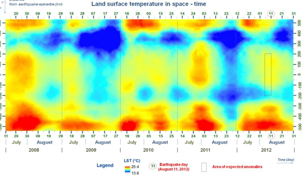
As the coordinate frame was established, 4102 points representing 26 locations for July and August for the period 2008-2012 with LST data were mapped onto it. A surface of the LST was then generated using Ordinary Kriging interpolation method. The created map (Figure 6) will be useful to investigate possible high LST values around the epicentre a few days before August 11, 2011, the day of the earthquake.
3.4.
Approach 2: detecting anomalous differences between land surface and
near-ground air temperature
“As solar energy strikes the earth’s surface each morning, a shallow (1–3 cm) layer of air directly above the ground is heated by conduction. Heat exchange between this shallow layer of warm air and the cooler air above is very inefficient. On a warm summer’s day, for example, air temperatures may vary by 15°C from just above the ground to waist height.” (Hackworth, 2004)
14
Therefore, night-time LST and air temperature datasets collected from 26 stations with weather sensors mounted 2 m above the ground were used as the input data for this second approach. In more details, these two datasets are described in sections 2.1.1 and 2.1.2 respectively.
The air temperature measured by each of the 26 weather stations daily for July and August during the period 2008-2012 was extracted. Along with the air temperature, the spatial LST mean of a 4 km2 area around each of the locations of the 26 weather stations was calculated for all the images of July and August during the period 2008-2012.
Similarly to LST changes, here we are also interested to detect possible anomalous temperature differences in time relative to the day of the earthquake and in space relative to the epicentre. Therefore, the need to build a space-time coordinate system emerges again. The same coordinate frame as in “Approach 1” was established. As in “Approach 1” the coordinate frame features time in days in the horizontal axis and epicentral distance in km in the vertical axis.
The only difference from “Approach 1” is that instead of LST, this time the difference between LST and air temperature 2 m above was plotted onto the space-time coordinate system. This system is described as in equation (3.2).
(3.2)
Where:
t- time in days starting from July 11, 2008 regarded as the horizontal axis
d –station of the station from the epicentre in km taking positive values for the stations north of the epicentre and negative for the stations in the south regarded as vertical axis
– difference in temperature between the land surface and air 2 m above, regarded as attribute
In order to preserve the space at its maximum, as in “Approach 1”, the geographical area was divided into two sections, north and south. The station distances from the epicentre belonging to the stations in the north were assigned positive values while the ones located south were assigned negative values. The temperature differences between land and air are described in (3.3).
(3.3)
Where:
- LST of a 4 km2 area around the weather station
- Air temperature measured by the weather station 2 m above ground
15
compared with the maps of other methods to analyze the degree that the temperature changes are matching in time.
3.5.
Approach 3: detecting temperature changes in the vertical atmospheric
column above the earthquake epicentre
In the third approach the investigated phenomena is going to be the air temperature of the atmospheric layers. As it might be implied by the research questions, there are two reasons for analyzing the atmosphere temperature: (a) To understand the weather effect on the temperature patterns found in “Approach 1” and “Approach 2”, and to compare these patterns with patterns in other periods; and (b) To analyze the temperature of the atmospheric boundary layer (the atmospheric layer extended 0.3-1 km above ground) for possible anomalous patterns caused by radon ionization.
The data used in this approach include the period from July, 11 to August 31, for the years 2007, 2008, 2010-2012. The timeline of the data aligns with the LST and air temperature data with the difference that year 2009 was traded for 2007 due to a 75% lack of atmospheric layer data during the former one. The observations are taken every day within the aforementioned period. In more details, the acquisition of the data and quality assurance processes are described in sections 2.1.3 and 2.2.3 respectively.
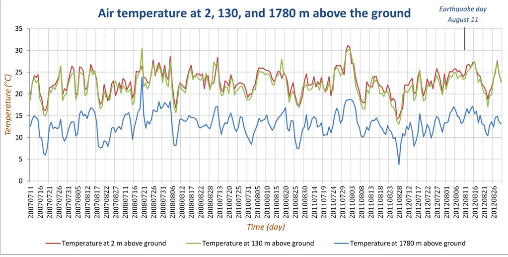
In order to investigate the temperature of the lower atmosphere, first, a two-dimensional graph was constructed with time horizontally and temperature vertically. Only the temperature measured at three different atmospheric levels over time was used to build the two-dimensional graph in order to show temperature trends at great detail for the lower atmosphere. The temperature measured daily at 2, 130, and 1780 m above the ground level was visualized through this graph (Figure 8).
Besides this time-temperature graph, another representation was made by visualizing the temperature starting from 2 m above ground, up to 30 km reaching the troposphere layer. The data were formatted to be consistent with a time-altitude coordinate frame. Time in days was mapped in the horizontal axis and altitude in km in the vertical one. All the points of the 5-year period were then mapped onto the coordinate frame. A temperature surface was generated using Ordinary Kriging interpolation method (Figure 9).
4.
Results and discussion
4.1.
Land surface temperature changes in space and time
16
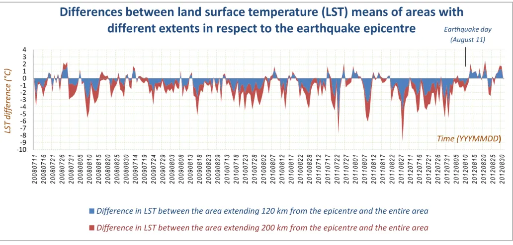
(a) The first graph (Figure 5) represents the LSTs differences among areas of different extent relative to the epicentre. Positive values indicate a rise in temperature of the area around the earthquake epicentre. Several positive values can be observed along the graph. However, no anomalous values are observed prior to the earthquake day. The highest values of the entire period in the graph are the ones occurring two days after the earthquake. Even if these high values have a relation with the earthquake, they are not in the form of a precursor and therefore they are of no interest for predictive activities. A similar behaviour of LST could be observed after the LST graphs between the area extending at a 120 km radius around the epicentre and the bigger area at a 200 km radius around the epicentre were compared. High values in the 120 km radius area correspond to the high values of the 200 km radius area and vice-versa. This parallelism indicates that the area located 120 km around the epicentre did not experience higher LST values than the 200 km radius area.
19
Figure 5: Differences in LSTs of areas with different extents relative to the earthquake epicentre. Positive values indicate higher land surface temperature of the areas close to the earthquake compared to the entire area. No anomalies exist a few days before the earthquake.
-10 -9 -8 -7 -6 -5 -4 -3 -2 -1 0 1 2 3 4
20080711 20080716 20080721 20080726 20080731 20080805 20080810 20080815 20080820 20080825 20080830 20090714 20090719 20090724 20090729 20090803 20090808 20090813 20090818 20090823 20090829 20100713 20100718 20100723 20100728 20100802 20100807 20100812 20100817 20100822 20100828 20110712 20110717 20110722 20110727 20110801 20110807 20110812 20110817 20110822 20110827 20120711 20120716 20120721 20120726 20120731 20120805 20120810 20120815 20120820 20120825 20120830
LS
T
d
if
feren
ce
(°
C)
Time (YYYMMDD
)
Differences between land surface temperature (LST) means of areas with
different extents in respect to the earthquake epicentre
Difference in LST between the area extending 120 km from the epicentre and the entire area
Difference in LST between the area extending 200 km from the epicentre and the entire area
20
21
4.2.
Anomalous temperature differences between land surface and
near-ground air
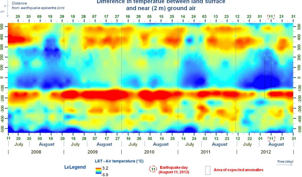
The result of this approach is an Ordinary Kriging surface featuring the differences in temperature between land and air 2 m above it. The resulted graph is shown in Figure 7. Again, our focus area is located 2-6 days before the earthquake at a spatial extent of 100 – 200 km from the epicentre represented with a dashed black rectangle shown in the graph. As it can be seen from the graph, the focus area exhibits a pattern of low values, the lowest within the period and within its spatial extent. In other words, the air temperature around the epicentre a few days before the earthquake has had the highest value within the entire period compared to the land surface temperature. If a source other than air was heating the land surface, according to M. Hackworth as explained in section 1.3.3,
21
21
4.3.
Temperature changes in the vertical atmospheric column above the
earthquake epicentre
The visualization of the temperature observations for multiple layers of the atmosphere helped understanding the weather effect over the temperature behaviour. As it was mentioned before, a temperature increase before earthquakes might also be caused by radon ionization, a process that is supposed to happen before earthquakes at the atmospheric boundary layer extending up to 1 km above ground. Therefore, it was also sought for localized temperature patterns caused by radon ionization at the lower levels of the atmosphere.
Two results in form of two graphs are the outputs of this approach. The first graph (Figure 8) features the air temperature for three different heights, 2, 130 and 1780 m above the ground for July and August during 2007, 2008, 2010-2012. There is no particular anomalous behaviour observed from the graph. The temperature follows the same trend along all three different altitude levels in the days prior the earthquake. This similarity suggests that there is not any localized warm pattern caused by radon ionization.
23
Figure 8: Daily air temperature measured at 3 different atmospheric levels. Temperature exhibits a normal behaviour in the days before the earthquake. All the three levels show similar trends. The graph was created using weather balloon radiosonde night time daily temperature observations.
0 5 10 15 20 25 30 35
20070711 20070716 20070721 20070726 20070731 20070805 20070812 20070817 20070822 20070827 20080711 20080716 20080721 20080726 20080731 20080806 20080812 20080817 20080822 20080828 20100713 20100720 20100725 20100731 20100805 20100810 20100815 20100820 20100825 20100830 20110714 20110719 20110724 20110729 20110803 20110808 20110813 20110818 20110823 20110828 20120712 20120717 20120722 20120727 20120801 20120806 20120811 20120816 20120821 20120826
Tem
p
era
tu
re
(°
C)
Time (day)
Air temperature at 2, 130, and 1780 m above the ground
Temperature at 2 m above ground Temperature at 130 m above ground Temperature at 1780 m above ground
24
Figure 9: Air temperature of the vertical atmospheric column. The white dots indicate that the warm pattern originated earlier in the high atmosphere to propagate later down to the lower layers. The graph was created using weather balloon radiosonde night-time daily temperature observations.
25
Furthermore, another observation can be made by looking at Figure 9. As indicated by the dashed white arrow line, the temperature increase propagates from higher to lower levels of the atmosphere through time. This suggests that the temperature increase originated from the higher atmosphere. Therefore, this approach also concludes that the LST increase detected after the earthquake event in first approach is due to the weather and because of a heating source coming from underground or the ground surface.
4.4.
Discussion
In contrast to the majority of studies that do recognize the existence of land surface temperature increase before big earthquakes, this study gave arguments supporting the opposite. This study can therefore be considered as a counterexample that would reject the general proposition which states that big earthquakes exhibit positive land surface temperature changes before they strike. This would bring out implications regarding the feasibility of setting up earthquake prediction systems in the domain of thermal precursors.
If an earthquake thermal-based prediction system existed and was up and running in the area where the earthquake of August 11, 2012 struck, the event would have been overlooked. The undertaken approaches in this research were able to detect anomalies, but not in form of precursors. As all the result showed, LST anomalies did not occur in the few days preceding the earthquake, but after the earthquake struck. Therefore, an earthquake prediction system would signal false detections in terms of time by therefore missing out the real event.
The techniques used in this research showed that the post-earthquake temperature increase was due to weather. This was accomplished by looking at the temperature patterns horizontally along the earth’s surface and also vertically through the atmosphere. These patterns had similar extent in time and space with patterns found in the other years. The weather origin of the temperature patterns however, does not confirm that temperature and earthquakes are unrelated at all. There might be a relation between thermal precursors and earthquakes, but this relation is weak enough to be masked by weather which is the primary factor of the temperature variations for both the atmosphere and the land surface.
Another obstacle that weakens the feasibility of relating thermal signals to earthquakes is the poor understanding of the mechanism of how thermal precursors emerge. Incomplete explanations are given to how an incoming earthquake triggers the temperature to increase. In efforts to understand the mechanism of how temperature propagates up to the land surface, an important finding from micrometeorology literature was made (Figure 10).
26
Figure 10: Diurnal soil temperature at different depth showing a very slow propagation (Arya, 2001). It can be implied that earthquake-related temperature propagations from underground to the land surface are very improbable.
Figure 10 shows the diurnal soil temperature variations at different depth. If we investigate the difference in time between the peak of the temperature measured at 2.5 cm depth and the peak measured at 15 cm, this difference is 4 hours. In other words, the temperature travels vertically through soil with a speed of 12.5 cm in 4 hours, or 3 meters in 4 days.
Furthermore, the speed of 3 meters in 4 days assumes that the temperature would not lose its magnitude while travelling through soil, which is not true. We have to consider the temperature attenuation effect to have a clearer view of how probable it is for the temperature to reach the land surface from underground. To illustrate this, we look at Figure 10 one more time. We can see that in contrast to the temperature at 2.5 cm underground which exhibits sharp peaks, the one at 30 cm experiences very slight variations. That means the temperature has attenuated while travelling downward. Adding the attenuation effect to the slow propagation, we can imply that insignificant amounts of temperature if not at all, would reach the land surface.
27
Having discussed the phenomena that are believed to be the origin of land surface thermal precursors by previous research and experiments, an important insight can be derived about their nature. All of the proposed thermal changes are effects of some causes. Investigating the cause rather than its effect would most likely give better results. The increase of well water levels for example is supposed to cause the increase of the LST. However, LST variations are primarily caused by weather. Therefore, it would be a more straightforward approach to measure well water levels instead of LST. Another example is the LST increase from radon ionization in soil (Pulinets et al., 2006). Similarly, it would be more significant to measure radon directly instead of LST. Indeed, there are studies that have been done on these other earthquake precursors as well. They also continue to be a big question on the earthquake prediction arena.
As it was underlain in the discussion paragraphs above, earthquake prediction in general continues to be a hot topic and thermal precursors are just one of the phenomena claimed to have a relation with earthquakes. Research on earthquake precursors is abundant and often the phenomena seem to be well understood. However, setting up prediction systems keeps causing a lot of drawbacks in the scientific community.
5.
Conclusions
The results derived by all three approaches were found to be consistent with each-other. After having summarized and interpreted these results, it was concluded that the hypothesised presence of land surface temperature anomalies a few days before the earthquake of August 11, 2012 was indeed false. In contrast to our hypothesis, the land surface temperature increase occurred two days after the earthquake, and not before it.
Besides the conclusion that the land surface did not experience any precursory temperature anomalies, the performed analyses also brought other conclusions explaining the source of the temperature patterns found after the earthquake struck. After having investigated the behaviour of both the land surface and the air temperature through time, it was reasoned out that the high temperature patterns found after the day of the earthquake for both air and land surface, were caused by the weather. The reason behind this conclusion is that both the air and the land surface temperature patterns occurred in similar spatial extents through different years in approximately the same period of the year. Furthermore, the land surface and near-ground air temperature patterns matched in time with the temperature patterns that were found using air temperature observations of multiple atmospheric levels. The atmospheric temperature patterns themselves exhibited similar vertical extent through time. This would weaken even more the relation of the land surface temperature increase with the earthquake even if the land surface would have experienced temperature anomalies. All of these indicators suggest that the temperature variations were seasonal.
28
In addition to the conclusions drawn above regarding the existence of the land surface and air thermal precursors, this study was also able to shed light on the mechanism of land surface temperature precursor by bringing up a soil layer temperature model from the literature (Figure 10). Having interpreted that model, it was concluded that the speed at which temperature propagates vertically through the soil, is very slow. Adding the attenuation effects, it would become very improbable for the temperature to reach the land surface from downward.
6.
Recommendations
The very first recommendation to be given to further studies concerning earthquake precursory temperature anomalies would be to analyze air temperature instead of land surface temperature. This is firstly because land surface temperature did not exhibit anomalies a few days before the earthquake while air temperature showed the highest anomaly of the entire under studied 5-year period in the few days before the earthquake, and secondly because temperature propagation through soil is extremely slow and too inefficient to be able to lead to land surface temperature increase for reasons other than weather. This second reasoning was discussed in section 4.4.
Second, a deeper understanding of weather behaviour is needed in order to say with more confidence if the anomalies in question are due to an incoming earthquake or an expected weather front. The reason why weather should be in the spotlight is because weather is the main and the most intense factor that causes temperature variations.
Third, careful interpretation should be made upon the apparent detected precursors. Anomalies always occur many times at multiple geographical regions. Making up random imaginary earthquakes along the under studied period and looking if anomalies precede them would give a more realistic perspective and it would help on quantifying how much accurate we can be in predicting earthquakes.
Lastly, adding to the above recommendations, more earthquakes would give more solid results and would determine if it is worth to consider the temperature as an earthquake precursor with the nowadays available measurement technologies and setups.
7.
References
ALIANO, C., CORRADO, R., FILIZZOLA, C., GENZANO, N., PERGOLA, N. & TRAMUTOLI, V. 2008. Robust TIR satellite techniques for monitoring earthquake active regions: limits, main achievements and perspectives. Annals of Geophysics, 51, 303-317.
ARYA, P. S. 2001. Introduction to micrometeorology, Academic press.
CICERONE, R. D., EBEL, J. E. & BRITTON, J. 2009. A systematic compilation of earthquake precursors.
Tectonophysics, 476, 371-396.
GARRATT, J. R. 1994. The atmospheric boundary layer, Cambridge university press.
GELLER, R. J. 2007. Earthquake prediction: a critical review. Geophysical Journal International, 131,
425-450.
HACKWORTH, M. 2004. Weather & Climate [Online]. Available:
http://www.physics.isu.edu/weather/kmdbbd/notesc3.pdf [Accessed 10/01/2013 2013]. IGARASHI, G. & WAKITA, H. 1991. Tidal responses and earthquake-related changes in the water level
29
LISI, M., FILIZZOLA, C., GENZANO, N., GRIMALDI, C., LACAVA, T., MARCHESE, F., MAZZEO, G., PERGOLA, N. & TRAMUTOLI, V. 2010. A study on the Abruzzo 6 April 2009 earthquake by applying the RST approach to 15 years of AVHRR TIR observations. Nat. Hazards Earth Syst. Sci, 10, 395-406.
MACCHERONE, B. MODIS specifications
[Online]. National Aeronautics and Space Administration. Available:
http://modis.gsfc.nasa.gov/about/specifications.php [Accessed 20/01/2013 2013]. MARVIN, C. 1918. Monthly Weather Review, Washington.
MINDER, J. R., MOTE, P. W. & LUNDQUIST, J. D. 2010. Surface temperature lapse rates over complex terrain: Lessons from the Cascade Mountains. Journal of Geophysical Research, 115, D14122. NCDC. 2013. NCDC official homepage [Online]. Available: www.ncdc.noaa.gov [Accessed 24/02/2013
2013].
NOAA. 2013. NOAA official homepage [Online]. Available: www.noaa.gov [Accessed 24/02/2013 2013].
OKYAY, Ü. 2012. Evaluation of thermal remote sensing for detection of thermal anomalies as earthquake precursor. Master, New University of Lisbon.
OUZOUNOV, D., BRYANT, N., LOGAN, T., PULINETS, S. & TAYLOR, P. 2006. Satellite thermal IR phenomena associated with some of the major earthquakes in 1999–2003. Physics and Chemistry of the Earth, Parts A/B/C, 31, 154-163.
OUZOUNOV, D. & FREUND, F. 2004. Mid-infrared emission prior to strong earthquakes analyzed by remote sensing data. Advances in Space Research, 33, 268-273.
PORSTENDÖRFER, J., BUTTERWECK, G. & REINEKING, A. 1991. Diurnal variation of the concentrations of radon and its short-lived daughters in the atmosphere near the ground. Atmospheric Environment. Part A. General Topics, 25, 709-713.
PULINETS, S., OUZOUNOV, D., KARELIN, A., BOYARCHUK, K. & POKHMELNYKH, L. 2006. The physical nature of thermal anomalies observed before strong earthquakes. Physics and Chemistry of the Earth, Parts A/B/C, 31, 143-153.
SARAF, A. K., RAWAT, V., CHOUDHURY, S., DASGUPTA, S. & DAS, J. 2009. Advances in understanding of the mechanism for generation of earthquake thermal precursors detected by satellites.
International Journal of Applied Earth Observation and Geoinformation, 11, 373-379. SCHOLZ, C. H. 2002. The mechanics of earthquakes and faulting, Cambridge university press.
SINGH, M., KUMAR, M., JAIN, R. & CHATRATH, R. 1999. Radon in ground water related to seismic events. Radiation measurements, 30, 465-469.
TORBATI, Y. 2012. Reuters. Available: http://www.reuters.com/article/2012/08/12/us-iran-earthquake-idUSBRE87A08N20120812 [Accessed 20/01/2013 2013].
TRAMUTOLI, V., DI BELLO, G., PERGOLA, N. & PISCITELLI, S. 2001. Robust satellite techniques for remote sensing of seismically active areas.
USGS. 2013. USGS official homepage [Online]. Available: www.usgs.gov [Accessed 24/02/2013 2013].
WAN, Z. 2006. MODIS land surface temperature products users' guide. Institute for Computational Earth System Science, University of California, Santa Barbara, CA. http://www. icess. ucsb. edu/modis/LstUsrGuide/usrguide. html.