Universidade Federal de São Carlos
Centro de Ciências Exatas e de Tecnologia
Departamento de Estatística
Time series forecasting:
advances on Theta method
José Augusto Fiorucci
Time series forecasting:
advances on Theta method
Tese apresentada ao Programa de Pós-Graduação em Estatística da Universidade Federal de São Carlos - PPGEs/UFSCar, como parte dos requisitos para
obtenção do título de Doutor em Estatística.
Orientador: Prof. Dr. Francisco Louzada Neto
Ficha catalográfica elaborada pelo DePT da Biblioteca Comunitária UFSCar Processamento Técnico
com os dados fornecidos pelo(a) autor(a)
F521t
Fiorucci, José Augusto
Time series forecasting : advances on Theta method / José Augusto Fiorucci. -- São Carlos : UFSCar, 2016.
87 p.
Tese (Doutorado) -- Universidade Federal de São Carlos, 2016.
Agradecimentos
Agradeço primeiramente a Deus por me permitir estudar e desenvolver pesquisas. Agradeço a toda minha família pelo apoio e incentivo, em especial aos meus pais, José Airton Fiorucci e Luzia Neuza Dalaqua, com os quais eu sempre estarei em divida. Agradeço ao meu orientador, Francisco Louzada Neto, por todo ensinamento, amizade e paciência durante esses anos.
Agradeço ao meu supervisor no exterior, Dipak Dey, o qual tornou possível o meu estágio nos Estados Unidos.
Agradeço aos muitos amigos pelos momentos de descontração e apoio. Em especial a Yiqi Bao, por todo convívio e colaboração durante esses anos.
Aos professores Ricardos Sandes Ehlers e Liane Werner, membros da banca de qualificação, pelas valiosas sugestões feitas.
Aos professores Adriano Kamimura Suzuki, Luis Aparecido Milan, Marinho Gomes de Andrade Filho e Rodrigo Fernandes de Mello, membros da banca de defesa, por todas correções e suggestões para trabalhos futuros.
Essa tese contou com a colaboração de varias pessoas com as quais sou extremamente grato. Em especial destaco meus coautores: Tiago Pellegrini, por ter me introduzido a trabalhar com o método theta e ter compartilhado varias ideias; Fotios Petropoulos, por todo acompanhamento e colaborações, as quais foram fundamentais para obtenção dos resultados aqui apresentados; Anne B. Koehler, por todas as correções, ideias e refinamentos.
Aos professores e aos demais funcionários do departamento de estatística da UFSCAR e da UCONN por todo ensinamento e excelente convívio.
I thank God for enabling me to study and develop this research.
I thank my family for their support and encouragement, especially, my parents, José Airton Fiorucci and Luzia Neuza Dalaqua, to whom I will always be indebted.
I thank my supervisor, Francisco Louzada Neto, for his teaching, counsel, friendship and patience.
I thank my external supervisor, Dipak Dey, who made my internship in the United States of America possible.
I thank my friends for shared moments and encouragement, in particular, Yiqi Bao, for her conviviality and cooperation.
I thank the Professors Ricardo Sandes Ehlers and Liane Werner, the members of my qualifying exam, for their invaluable recommendations.
I thank the Professors Adriano Kamimura Suzuki, Luis Aparecido Milan, Marinho Gomes de Andrade Filho and Rodrigo Fernandes de Mello, the member of my defense exam, for all corrections and suggestions for future works.
This PhD thesis was developed with the collaboration of several colleagues, to whom I am most grateful, above all, my coauthors: Tiago Pellegrini, who introduced me to Theta methods and shared several ideas; Fotios Petropoulos, whose contributions were critical to obtaining the results reported herein; Anne B. Koehler, for all corrections, ideas and improvements.
I wish to express my gratitude to the professors and other staffs in the department of statistics at UFSCAR and UCONN for their teaching and congeniality.
Resumo
Métodos precisos e robustos para prever séries temporais são muito importantes em diversas áreas. Uma vez que os dados históricos são utilizados para o planejamento estratégico de operações futuras, como compra ou venda de determinados produtos para controle de estoque e demanda.
Neste contexto, várias competições para métodos de previsão de séries temporais univariadas foram realizadas, sendo a Competição M3 a maior. Ao vencer a Competição M3, o método Theta intrigou pesquisadores por sua capacidade preditiva e simplicidade. O método Theta é uma combinação de outros métodos, o qual propõe decompor a série temporal (desazonalizada) em outras duas séries temporais chamadas de "linhas thetas". A primeira linha theta remove completamente a curvatura dos dados, sendo assim um estimador para a tendência a longo prazo. A segunda linha theta dobra a curvatura da série sendo assim um estimador para a componente de curto prazo.
Várias questões relacionadas ao método Theta foram levantadas, algumas pelos próprios autores, como parâmetros ideais para as linhas thetas, pesos para combinar as linhas thetas, construção de intervalos de predição, número ideal de linhas thetas, entre outras.
Nesta tese algumas dessas questões são solucionadas. Pesos ótimos para a combinação de linhas thetas são derivados, esses resultados são utilizados para a construção de modelos estatísticos que generalizam/aproximam o método Theta padrão. A metodologia estatística é empregada para estimação dos parâmetros e construção de intervalos de predição. Os pesos ótimos também são utilizados para propor métodos que consideram duas ou mais linhas thetas. Parte da metodologia proposta é implementada em um pacote para a linguagem de programaçãoR.
Accurate and robust forecasting methods for univariate time series are critical as the historical data can be used in the strategic planning of such future operations as buying and selling to ensure product inventory and meet market demands.
In this context, several competitions for time series forecasting have been organized, with the M3-Competition as the largest. As the winner of M3-Competition, the Theta method has attracted attention from researchers for its predictive performance and simplicity. The Theta method is a combination of other methods, which proposes the decomposition of the deseasonalized time series into two other time series called "theta lines". The first completely removes the curvatures of the data, thus accurately estimating the long-term trend. The second doubles the curvatures to better approximate short-term behavior.
Several issues have been raised about the Theta method, even by its originators. They include the number of theta lines, their parameters, weights to combine them, and construction of prediction intervals, among others.
This doctorate thesis resolves part of these issues. We derive optimal weights for combine the theta lines, this result is used to derive statistical models which generalizes /approximate the standard Theta method. The statistical methodology is considering for parameter estimation and for compute the prediction intervals. The optimal weights are also used to propose new methods that hold two or more theta lines. Part of proposed methodology is implemented in a package for R-programming language.
Contents
Contents . . . . v
List of Figures . . . . vii
List of Tables . . . . 0
1 INTRODUCTION . . . . 1
1.1 Chapters descriptions . . . 2
2 SYSTEMATIC REVIEW . . . . 3
2.1 Introduction . . . 4
2.2 Content analysis methodology . . . 4
2.3 Results and discussion . . . 8
2.4 Final comments . . . 11
3 MODELS FOR OPTIMISING THE THETA METHOD . . . . 17
3.1 Introduction . . . 18
3.2 Theta method and SES-d . . . 20
3.2.1 The original Theta method . . . 20
3.2.2 SES with drift . . . 21
3.2.3 Other generalisations of Theta method . . . 22
3.3 Models for Optimising the Theta Method . . . 23
3.3.1 Optimised Theta Model and Standard Theta Model . . . 24
3.3.2 Dynamic Optimised Theta Model and Dynamic Standard Theta Model . . 25
3.3.3 Parameter estimation . . . 26
3.4 Empirical evaluation . . . 27
3.4.1 Design . . . 27
3.4.2 Results . . . 29
3.4.3 Discussion . . . 32
3.5 Concluding remarks . . . 34
4 EXPANDING THE THETA METHOD . . . . 39
4.2.2 Three theta lines . . . 43
4.2.3 Four or any even number of theta lines . . . 45
4.2.4 Definitions of methods and estimation of theta parameters . . . 46
4.3 Application to M3 database. . . 49
4.4 Final Comments . . . 52
5 FORECTHETA R PACKAGE . . . . 55
5.1 Introduction . . . 56
5.2 Theta Models . . . 57
5.3 Generalised Rolling Origin Evaluation . . . 58
5.4 The forecTheta R package . . . 59
5.4.1 The time series forecasting functions . . . 59
5.4.2 The cross validation functions . . . 62
5.4.3 Other functions. . . 63
5.4.4 Illustrations . . . 64
5.4.5 DOTM behavior for artificial data . . . 66
5.4.6 Reproducing the DOTM results for M3 data set . . . 71
5.5 Final comments . . . 72
6 CONCLUSION . . . . 73
List of Figures
Figure 1 – Procedure of the content analysis review. . . 5
Figure 2 – Number of articles per year. . . 9
Figure 3 – MCB intervals for selected forecasting methods. . . 33
Figure 4 – Representation of the solution line (non-dashed line) for the three theta lines method in the casesθ2 ≤1 andθ2>1, where the middle point is highlighted with a star point. . . 44
Figure 5 – Example of fixed origin evaluation. The model is fitted in the training sample part and predictions (blue line) are computed for validation sample part. In gray are present the errors of prediction. . . 48
Figure 6 – MCB intervals with 95% of confidence. . . 52
Figure 7 – Example of GROE function. . . 60
Figure 8 – Example of plot(dotm(y,8)) command. . . 66
Figure 9 – DOTM behavior for simulated data. . . 69
Table 1 – List of questions and possible responses to the proposed content analysis 6 Table 2 – Number of papers per journal and main objective of published papers. 9
Table 3 – Authors with more than 3 papers and at least 1 as first co-author. . . . 10
Table 4 – Summary of reviewed articles according to the content analysis (1995– 2015) . . . 12
Table 5 – Indexing of reviewed articles (2014-2015) . . . 14
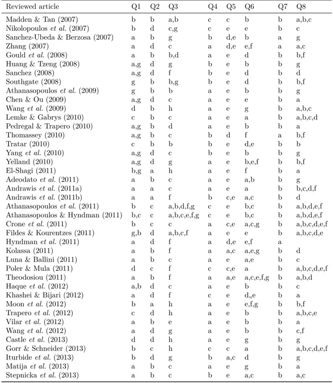
Table 6 – Indexing of reviewed articles (2007-2013) . . . 15
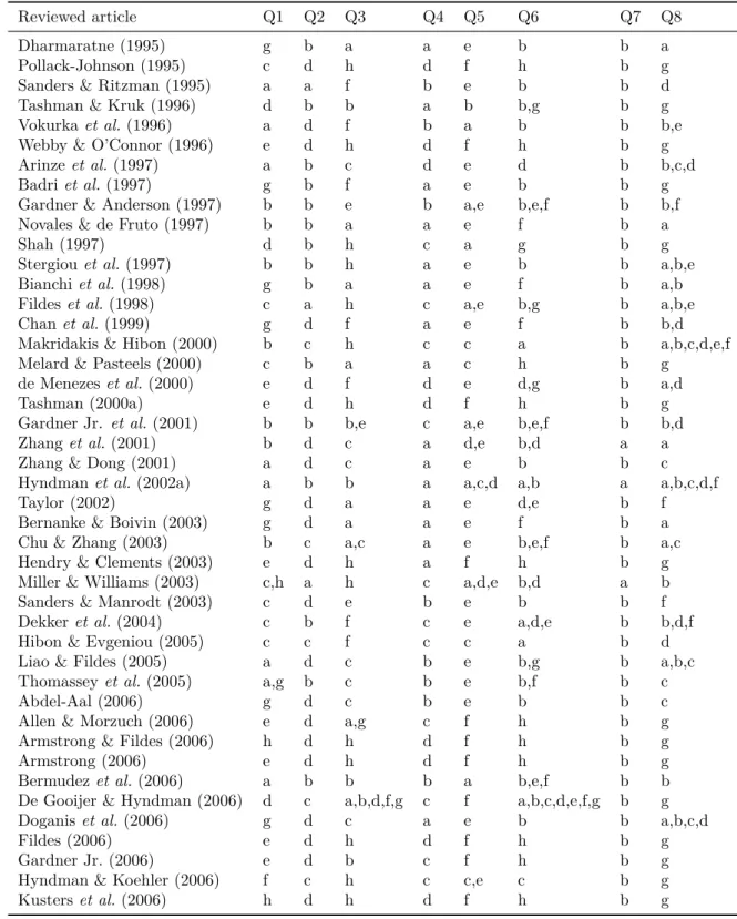
Table 7 – Indexing of reviewed articles (1995-2006) . . . 16
Table 8 – The different Theta methods and models considered in the empirical evaluation. . . 27
Table 9 – The benchmark methods used in the current study. . . 28
Table 10 – M3-Competition dataset. . . 28
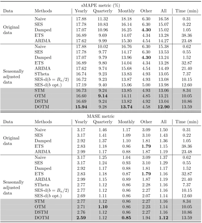
Table 11 – Empirical results for all methods using the sMAPE and the MASE. . . 30
Table 12 – Empirical results for SES-d (boptimised) and OTM for the trimmed sMAPE. . . 32
Table 13 – Percentage improvements for DOTM over DSTM in terms of MASE (numbers in brackets refer to sample sizes). . . 33
Table 14 – Empirical results for all methods using the sMdAPE. . . 38
Table 15 – The weights (ω1∗, ω2∗) for the method with two theta lines fixing θ1 = 0. 43 Table 16 – The weights (ω∗ 1, ω∗2, ω∗3) for the method with three theta lines fixing θ1 = 0. . . 45
Table 17 – The weights (ω1∗, ω∗2, ω∗3, ω∗4) for the method with four theta lines fixing θ1 = 0. . . 46
Table 18 – M3-Competition data set. . . 49
Table 19 – The benchmark methods used in the current study. . . 50
Table 20 – Selected theta values using the in-sample sMAPE metric for M3 data set. 51 Table 21 – Empirical results for out-sample sMAPE metric for all methods. . . 51
Table 22 – In-sample sMAPE results forLS(θ1, θ2). . . 53
Table 23 – In-sample sMAPE results forLDS(θ1, θ2, θ3). . . 53
Table 24 – In-sample sMAPE results forLDDS(θ1, θ2, θ3, θ3). . . 54
1 Introduction
This study focuses on time series forecasting models, especially, those for univariate time series. The application of these models extends through several areas of economy, commerce, energy, and health for which historical data regarding transactions, prices, demand, customers/patients, and other factors can provide predictive value in logistics planning.
In search of the optimal forecasting method, several competitions have been organized. Among the most significant are the Makridakis Competitions organized by the Inter-national Institute of Forecasters, which began in 1982 with the M-Competition, which comprised 24 competitors and 1001 time series. In 1993, the M2-Competition included 19 competitors and 29 time series. The largest competition to date, the M-3 Competition, took place in 2000 with 24 competitors and 3,003 time series, involving macro- and micro-economy, industry, finance and demographics. The time series were distributed with frequencies of yearly, quarterly, monthly and other (including daily and weekly) observations. The results were published in the International Journal of Forecasting (Makridakis and Hibon, 2000). The principal findings of the three competitions are
similar, the most significant are the following:
• Sophisticated methods do not ensure greater accuracy than simple ones;
• The accuracy measure may influence the ranking of performance of various methods;
• On average The combination of methods outperforms the specific methods being combined;
• The ranking of various methods vary according the length of forecasting horizon;
exponential smoothing, respectively. All details about the Theta method will be present in Chapter 3.
This thesis expands the theory of time series forecasting, particularly as it concerns the Theta method. A systematic review of more than 100 related studies published over the last two decades is presented, with a questionnaire used to identify each study’s primary objective and classify its methodology. The findings were used to analyze the evolution of related literature and determine the present state of research.
The principal advances in the Theta method expand the number of theta lines, compute optimal weights for combining them, derive stochastic approaches, and use statistical theory to estimate parameters and establish prediction intervals. The new models perform quite well using the M3-Competition data, with some outperforming the standard Theta method according to two well-established metrics and a statistical test. The code implementation of the proposed models via theforecTheta package for
R-programming language has been made freely available.
1.1
Chapters descriptions
The remainder of this study is organized as follows. The research is reported in four papers, with a chapter devoted to each. The first (Chapter 2), systematically reviews time series forecasting literature over the past two decades, considering more than 100 studies and addressing several questions for each. Chapter 3 presents the paper "Models for optimising the theta method and their relationship to state space models," which has been accepted for publication in the International Journal of of Forecasting. In that study, optimal weights for combining two theta lines were established and used to derive four stochastic approaches for the Theta method. The most elaborate model is the Dynamic Optimized Theta (DOTM), which performs well using M3-Competition data. Chapter 4 provides conditions to combine two or more theta lines with optimal weights, which are determined for three or any even number of theta lines and used to expand the standard Theta method to three or four theta lines. The study’s results show that increasing the number of theta lines enhances forecasting accuracy.
2 Systematic review for time series
fore-casting
This chapter corresponds to a manuscript to be submitted to a scientific journal, which presents a systematic review for time series forecasting involving more than one hundred of papers. The people involved in this work are: Bao Yiqi (Federal University of São Carlos, Brazil), Francisco Louzada (University of São Paulo, Brazil) and Dipak Dey (University of Connecticut, USA).
Abstract
2.1
Introduction
Time series analysis has significant application into such key areas as the economy, engineering, commerce, and health. The study of time series modeling, in turn, involves such fields of knowledge as mathematics, statistics, and computer science, with a focus on forecasting. Forecast-related literature has been growing rapidly over the last few decades (De Gooijer & Hyndman, 2006) as consequence of such factors as forecasting competitions (Makridakiset al., 1993; Makridakis & Hibon, 2000; Athanasopoulos et al., 2011), progress of automatic algorithms (Hyndmanet al., 2002a; Poler & Mula, 2011), and specialized computers softwares (Kusterset al., 2006; Hyndman & Khandakar, 2008). Even a series of studies focused on the same research topic generally has different objectives. Systematic review, content analysis or still scientometric analysis facilitate our understanding of a specific research area’s primary objectives, model classification, and comparison techniques. Moreover, this type of study enables us to analyze the evolution of the related literature, principal studies. and their authors’ academic affiliations.
This study has conducted a systematic review of the articles published over the past two decades covering all studies related to time series forecasting (TSF) included in the ScienceDirect and Scopus databases. The studies are classified under several categories such as publication year, journal title, year, first author, and primary objective. This study improves a better understanding about the historical evolution and the current state of this research area.
This chapter is organized as follows. Section 2.2 describes the methodology to select and classify study articles, while Section 2.3 discusses the results of their categorization. Final comments and recommendations for further research are presented in Section 2.4.
2.2
Content analysis methodology
The methodology used to select and classify the articles covered by this review is based on published papers of content analysis for other areas. Interested readers may refer to Li & Cavusgil (1995) and Hachicha & Ghorbel (2012) for more details.
All study is performed taking into account the online papers available onScienceDirect andScopusdatabases. The articles were found via computerized search related key words that follow the selection criteria:
CHAPTER 2. SYSTEMATIC REVIEW 5
Potentially related articles (124)
Articles selected in this survey
(109)
Exclusion of articles based on selection criterions
(15)
Classification and statistics Based on four categories
(1) Year of publication
(2) Title of journal
(3) Last name of the first co-author
(4) Conceptual scheme based on 8 questions
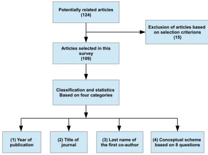
Figure 1 – Procedure of the content analysis review.
• The content analysis restricts the study eligibility to journal full articles in English. Other publication forms such as unpublished working papers, master and doctoral dissertations, books, conference in proceedings, white papers, and others were ineligible for inclusion.
The articles were selected and classified according to the procedure depicted in Figure 6. From 124 studies, 109 were selected with 15 failing to meet the selection criteria. Each was classified according to year of publications, title of journal, last name of the first co-author and other eight questions listed in Table 1. These questions were selected in order to identify the main proposes and how these proposes were presented in the articles. Some articles propose modifications on well established models, in these cases, we consider the result as a new model/methodoly. The study does not distinguish the terms "model" and "method" in regard to stochastic or deterministic processes.
This study considers eight types of primary objectives: those in which the study proposes a new method for TSF, compares traditional methods, discusses methods or techniques related TSF conceptually, proposes new features for model selection, reviews related literature, proposes a new feature for performance measurement, models a type of data set, and addresses other TSF-related issues not previously considered.
1. What is the main objective of the article?
a) Propose a new model/methodology
b) Comparison in methods
c) Conceptual discussion
d) Feature selection
e) Literature review
f) Performance measure
g) Application
h) Other issues
2. How is the seasonality modeled in the pro-posed/worked models?
a) Prior decomposition
b) Included in the model
c) Both
d) Not considered/Not apply
3. What is the type of the main classification method?
a) ARIMA
b) Exponential Smoothing
c) Neural networks
d) State Space Models
e) Non parametric approach
f) Combination
g) Other
h) Not apply
4. How are the considered methods?
a) Stochastic
b) Deterministic
c) Both
d) Not apply
5. What datasets are used?
a) M1-Competition
b) M2-Competition
c) M3-Competition
d) Simulated
e) Other
f) Not apply
6. Which metrics are considered?
a) sMAPE/sMdAP b) MAPE/MdAPE c) MASE/MdASE d) MSE/MdSE e) MAE/MdAE f) RMSE/RMdSE g) Other
h) Not apply
7. Was performed exhaustive simulation study?
a) Yes
b) No
8. Which benchmarks methods are considered for comparison?
a) ARIMA
b) Exponential Smoothing
c) Neural Network
d) Combination
e) Naive/Seasonal Naive
f) Other
g) Not apply/None
CHAPTER 2. SYSTEMATIC REVIEW 7 (e.g., classical decomposition) or included in the model (e.g., Holt-Winters) and type of the main method. We consider six family models as alternative, one example of combination type is the Theta Model of Assimakopoulos & Nikolopoulos (2000), the winner of the M3-Competition (Makridakis & Hibon, 2000). Question number (4) refers to stochastic or deterministic modeling of proposed or implemented methods. While the punctual forecasts are sometimes the same in both cases, the use of stochastic approaches has benefits, such as the possibility to use the information criteria for model selection and easy construction of prediction intervals.
The three M-Competitions have invaluable importance for TSF research and literature, see Makridakiset al. (1993); Makridakis & Hibon (2000) for details. The time series sets used in the competitions are freely available on Internet, researchers can use them to validate their methods and compare their performance. Question 5 identifies each data set, or part thereof, used in the studies, while Question 6 focuses on the metrics used to compare models. The customary metric used to this end is the MAPE defined as the mean of Absolute Percentage Errors (APE) given by
AP E(yt,ybt) = 100
|yt−ybt|
yt
,
whereytis true value one point of time series andybis the forecast fory. Absolute percent errors (APE), however, are not a symmetric function, which means that MAPE does not attend the mathematical restriction to be a true metric. Accordingly, the symmetric mean absolute percentage error (sMAPE) which is defined as the mean of symmetric absolute percentage errors (sAPE), is sometimes used in lieu of MAPE and is given by
sAP E(yt,ybt) = 100
|yt−ybt| (yt+ybt)/2
.
It is worth noting that sMAPE was the official metric of the M3-Competition. Although sAPE is a symmetric function and its correspondent mean is a true mathematical metric, sAPE does not treat positive and negative errors equally. Suppose, for example, thatyt = 100 soybt= 90 has bigger penalization than ybt = 110, while the variation in both cases is the same. Noting these problems, Hyndman & Koehler (2006) proposed the Mean Absolute Scaled Error metric (MASE) given by
M ASE = n−1
h
nX+h
t=n+1
|yt−ybt|
Pn
i=2|yi−yi−1|
,
Other alternatives are the mean square error (MSE), mean absolute error (MAE), and root mean square error (RMSE), which are not scale independent and thus unsuitable for comparisons with more than one time series. Variations using the median statistic of the same errors substitute "Md" for "M," e.g., the symmetric median absolute percentage error (sMdAPE).
Question 7 asks whether the researchers performed exhaustive simulation analyses, a traditional question in systematic reviews in diverse areas with limited available data. Time series analyses enables researcher to test their methods via empirical studies. By way of example, the M- and M3-Competition data sets have more than one and three thousand time series for this purpose, respectively.
Whenever researchers discover a new method, the customary practice is to compare it with well established methods serving an analogous purpose. Thus Question 8 identifies standard benchmark methods. Some alternatives coincide with those in Question 3. The naive model yields forecasting values equal to the last observed value, while its seasonal variation produces values equal to the last observed value of the same season. Questions 1, 3, 5, 6, and 8 allow more than one alternative answer per study.
2.3
Results and discussion
This section presents the results of the reviewed studies and discusses their classifica-tion. The results for each question are provided in the Appendix.
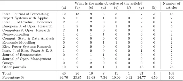
The number of published studies on time series forecasting is growing annually as evidenced by Figure 2, which shows a clear growth from 3 published studies in 1995 to 14 in 2014, the last full year. The 109 articles selected for this study are distributed among 39 journals. The International Journal of Forecasting (IJF) published 45 (41.3%), by Expert Systems with Applications and the International Journal of Production Economics, with 7 each, and the European Journal of Operational Research, with 5. The primary objective of the largest portion (36.7%) of the studies was proposing new forecasting methods or methodologies, while comparison in traditional methods and application are the focus of 23.85% and 24.77%, respectively. Table 2 shows the number of the articles per journal and the number of answers for each response to Question 1 in Table 1. Note that IJF is the only journal with at least one study for each objective.
CHAPTER 2. SYSTEMATIC REVIEW 9
Year
Number of ar
ticles
1995 1997 1999 2001 2003 2005 2007 2009 2011 2013 2015
2
4
6
8
10
12
14
Articles by year General trend
Figure 2 – Number of articles per year.
Table 2 – Number of papers per journal and main objective of published papers.
What is the main objective of the article? Number of (a) (b) (c) (d) (e) (f) (g) (h) articles Inter. Journal of Forecasting 12 13 9 3 8 1 7 5 45 Expert Systems with Applic. 6 0 0 1 0 0 2 0 7 Inter. J. of Produc. Economics 2 3 2 0 0 0 2 0 7 European J. of Oper. Research 1 2 0 0 1 0 2 0 5 Computers & Oper. Research 2 1 0 0 0 0 0 0 3
Neurocomputing 1 0 1 1 0 0 0 0 3
Comput. Stat. & Data Analysis 2 0 0 0 0 0 0 0 2
Economic Modelling 0 0 0 1 1 0 0 0 2
Elec. Power Systems Research 2 0 0 0 0 0 0 0 2 Inter. J. of Elec. Power & E. S. 1 0 0 0 0 0 1 0 2 Journal of Econometrics 0 0 1 1 0 0 0 0 2 Journal of Oper. Management 1 0 1 0 0 0 0 0 2
Omega 0 0 2 0 0 0 0 0 2
Other journals 10 7 0 1 1 0 13 0 25
Total 40 26 16 8 11 1 27 5 109
Percentage % 36.70 23.85 14.68 7.34 10.09 0.92 24.77 4.59 100
University authored the largest number of published studies, 10 and 6, respectively, representing 9.17% and 5.5% of the articles in this study, and both have been first authors of three.
Table 3 – Authors with more than 3 papers and at least 1 as first co-author.
Author Affiliation, Country Number of papers Number of
as first author papers
Hyndman, R.J. Monash University, Australia 3 10
Fildes, R. Lancaster University, United Kingdom 3 6
Athanasopoulos, G. Monash University, Australia 3 4
Gardner Jr., E.S. University of Houston,United States 3 3
Kourentzes, N. Lancaster University, United Kingdom 2 4
Hendry, D.F. University of Oxford, United Kingdom 2 3
Zhang, G.P. Georgia State University, United States 2 3
Andrawis, R.R. Cairo University, Egypt 2 2
Armstrong, J.S. University of Pennsylvania, United States 2 2
Sanders, N.R. Wright State University, United States 2 2
Tashman, L.J. University of Vermont, United States 2 2
Thomassey, S. University Lille Nord of France, France 2 2
Nikolopoulos, K. University of Manchester, United Kingdom 1 4
Hibon, M. INSEAD Business School, France 1 4
Petropoulos, F. Cardiff University, United Kingdom 1 3
Goodwin, P. University of Bath, United Kingdom 1 3
answers for each study can be found in Tables 5, 6, and 7 in the Appendix.
Note that (a), (b) and (g) to question (1) are the most common study objectives on the articles, appearing in an increasing number of published articles. The three objectives are related to proposing, modifying, or selecting specific models for specific time series. For example, several studies focused on producing economic energy models have been published in the last decade. Response (a) registered the highest increase in published articles from the first to the second period. We found very few articles related to feature selection, once the traditional statistical theory for model selection based in information criteria as AIC (Akaike, 1974), AICc and BIC (Schwarzet al., 1978) is very used in this issue. Only Hyndman & Koehler (2006), which proposed use of the mean absolute scaled error (MASE) metric, was classified as a performance measure. Responses to Question 2 indicate that, among studies addressing seasonal trends, models with built-in seasonal variables, are used most frequently.
CHAPTER 2. SYSTEMATIC REVIEW 11 classification method. The Question 4 shows that stochastic models are preferable by researches and the percentage increased in the last decade, however it is worth men-tioning that this is not one important issue for some practitioners of forecasting, since some models produce the same forecasting points for both stochastic or deterministic approaches, as occurs for exponential smoothing and ARIMA models for example.
Despite of importance of the M-Competitions for TSF, responses to Questions 5 indicate that no more than 25% of the study articles considered the data sets used in them. Often studies used time series classified as "Other", which generally represent just one specific kind of time series and not a set with several series from different areas. Moreover, just 8.26% of the studies used simulated data sets, the same number of articles that performs exhaustive simulation study (Question 7). Several metrics are considered in the articles and the distribution seems to be change over the last two decades by inclusion of a very specific metric for forecasting methods, the MASE. These results are shown in Question 6.
On Question 8 we can see the mostly frequent benchmarks methods in the articles, the ARIMA and Exponential Smoothing families are the most used. The automatic selection of ARIMA model proposed in (Boxet al., 2015, hereafter BJ-ARIMA) is, probably, the most used. However, particularly cases as auto-regressive models (AR) and moving average models (MA) are widely used as well. There is also the ETS (abbreviation of Error, Trend and Seasonal) algorithm for automatic selection of Exponential Smoothing (ES) model proposed by Hyndman et al. (2002b), which is not still so used as much as the particular ES cases, simple exponential smoothing (Brown, 1956) and Holt’s exponential smoothing (Holt Charles, 1957). Neural Network family is growing up fast, which coincides with the growing up of the number of papers dedicated to Neural Network model presented on Question 3 results. The other methods are still well used, this category includes several specific data set models and non parametric approaches.
2.4
Final comments
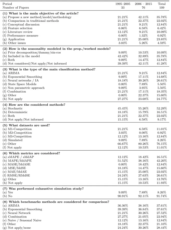
We presented in this paper a methodologically structured content analysis of time series forecasting literature over the last two decades. A total of 109 articles available in two well known databases, ScienceDirect and Scopus, were analyzed and classified for this study.
Table 4 – Summary of reviewed articles according to the content analysis (1995–2015)
Period 1995–2005 2006 – 2015 Total
Number of Papers 33 76 109
(1) What is the main objective of the article?
(a) Propose a new method/model/methodology 21.21% 42.11% 35.78% (b) Comparison in traditional methods 21.21% 22.37% 22.02% (c) Conceptual discussion 21.21% 9.21% 12.84%
(d) Feature selection 6.06% 6.58% 6.42%
(e) Literature review 12.12% 9.21% 10.09%
(f) Performance measure 0.00% 1.32% 0.92%
(g) Application 21.21% 25.00% 23.85%
(h) Other issues 3.03% 5.26% 4.59%
(2) How is the seasonality modeled in the prop./worked models?
(a) Prior decomposition/dummy/sin-cos 9.09% 10.53% 10.09% (b) Included in the model 42.42% 32.89% 35.78%
(c) Both 9.09% 14.47% 12.84%
(d) Not considered/Not apply/Not informed 39.39% 42.11% 41.28%
(3) What is the type of the main classification method?
(a) ARIMA 21.21% 9.21% 12.84%
(b) Exponential Smoothing 9.09% 17.11% 14.68% (c) Neural networks / IA 18.18% 30.26% 26.61%
(d) State Space Models 0.00% 7.89% 5.50%
(e) Non parametric approach 9.09% 3.95% 5.50%
(f) Combination 21.21% 17.11% 18.35%
(g) Other 0.00% 22.37% 15.60%
(h) Not apply 27.27% 23.68% 24.77%
(4) How are the considered methods?
(a) Stochastic 45.45% 55.26% 52.29%
(b) Deterministic 18.18% 15.79% 16.51%
(c) Both 21.21% 22.37% 22.02%
(d) Not apply/Not informed 15.15% 6.58% 9.17%
(5) What datasets are used?
(a) M1-Competition 21.21% 6.58% 11.01%
(b) M2-Competition 3.03% 0.00% 0.92%
(c) M3-Competition 12.12% 13.16% 12.84%
(d) Simulated 9.09% 7.89% 8.26%
(e) Other 66.67% 80.26% 76.15%
(f) Not apply 12.12% 10.53% 11.01%
(6) Which metrics are considered?
(a) sMAPE / sMdAP 12.12% 18.42% 16.51%
(b) MAPE/MdAPE 51.52% 38.16% 42.20%
(c) MASE/MdASE 0.00% 18.42% 12.84%
(d) MSE/MdSE 18.18% 14.47% 15.60%
(e) MAE/MdAE 15.15% 25.00% 22.02%
(f) RMSE/RMdSE 24.24% 27.63% 26.61%
(g) Other 15.15% 13.16% 13.76%
(h) Not apply 15.15% 10.53% 11.93%
(7) Was performed exhaustive simulation study?
(a) Yes 9.09% 7.89% 8.26%
(b) No 90.91% 92.11% 91.74%
(8) Which benchmarks methods are considered for comparison?
(a) ARIMA 36.36% 38.16% 37.61%
(b) Exponential Smoothing 39.39% 36.84% 37.61%
(c) Neural Network 21.21% 30.26% 27.52%
(d) Combination 27.27% 21.05% 22.94%
(e) Naive / Seasonal Naive 12.12% 13.16% 12.84%
(f) Other 18.18% 22.37% 21.10%
CHAPTER 2. SYSTEMATIC REVIEW 13 research is being conducted across the globe. The study articles were published in 39 scientific journals, most of which focus on a particular aspect of application. The significant role played by the International Journal of Forecasting is underscored by the fact that 43% of the study articles were published in its pages. The most common objective of the studies was to introduce a new forecasting method, often focused on a specific type of time series and most frequently classified as neural networks. Few studies conduct exhaustive simulation, while most use empirical data with one or more time series. ARIMA and Exponential Smoothing models are almost mandatory benchmarks methods for comparing performance, yet only one of the 109 studies focused on performance measurement as its primary objective, a research gap that merits attention. Non expert users should consider the automatic algorithms BJ-ARIMA and ETS as a first attempt to time series forecasting.
The study’s content analysis was exhaustive and, above all, productive, but limitations remain. Studies selected were limited to those published in English as complete journal articles and included in two prominent databases. While this generated a representative sample that served this study well, further research could included additional databases and criteria to expand the subject pool.
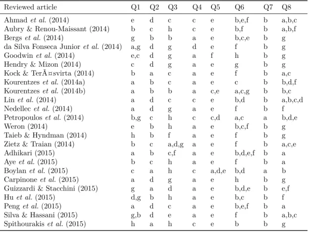
Table 5 – Indexing of reviewed articles (2014-2015)
Reviewed article Q1 Q2 Q3 Q4 Q5 Q6 Q7 Q8
Ahmadet al.(2014) e d c c e b,e,f b a,b,c
Aubry & Renou-Maissant (2014) b c h c e b,f b a,b,f
Bergset al. (2014) g b b a e b,c,e b g
da Silva Fonseca Junioret al. (2014) a,g d g d e f b g
Goodwinet al.(2014) e,c d g a f h b g
Hendry & Mizon (2014) c d g a e g b g
Kock & Teräsvirta (2014) b a c a e f b a,c
Kourentzeset al.(2014a) a b c a e c b b,d,f
Kourentzeset al.(2014b) a b b a c,e a,c,g b b,c Linet al.(2014) a d c c e b,d b a,b,c,d
Nedellecet al.(2014) a d g a e f b f
Petropouloset al. (2014) b,g c h c c,d a,c a b,d,e
Weron (2014) e b h a e b,c,f b g
Taieb & Hyndman (2014) h b f a e f b g
Zietz & Traian (2014) b c a,d,g a e f b a,c,e
Adhikari (2015) a b c,f a e b,d,e,f b a
Ayeet al.(2015) b c h a e f b a
Boylanet al. (2015) c a h c a,d,e b,d a b
Carpinoneet al.(2015) a d g a e h b g
Guizzardi & Stacchini (2015) g a d a e b,d,e b e,f Huet al. (2015) d,g b h a e b,c b f Penget al.(2015) a d c a e b,e,f b a
Silva & Hassani (2015) g,b d e a e f b a,b,c
CHAPTER 2. SYSTEMATIC REVIEW 15
Table 6 – Indexing of reviewed articles (2007-2013)
Reviewed article Q1 Q2 Q3 Q4 Q5 Q6 Q7 Q8
Madden & Tan (2007) b b a,b c c b b a,b,c
Nikolopouloset al.(2007) b d c,g c e e b c
Sanchez-Ubeda & Berzosa (2007) a b g b d,e b a g
Zhang (2007) a d c a d,e e,f a a,c
Gouldet al.(2008) a b b,d a e d b b,f
Huang & Tzeng (2008) a,g d g b e b b g
Sanchez (2008) a,g d f b e d b d
Southgate (2008) g b b,g b e d b b,f
Athanasopouloset al. (2009) g b b a e b b g
Chen & Ou (2009) a,g d c a e e b a
Wanget al.(2009) d b h a e g b a,b,c
Lemke & Gabrys (2010) c b c a e a b a,b,c,d
Pedregal & Trapero (2010) a,g b d a e b b a
Thomassey (2010) a,g b c b d f a b,f
Tratar (2010) c b b b e d,e b b
Yanget al.(2010) a,g d c b e b b g
Yelland (2010) a,g d g a e b,e,f b b,f
El-Shagi (2011) b,g a h a e f b a
Adeodatoet al.(2011) a b c a e a,b b g
Andrawiset al. (2011a) a a c a e a b b,c,d,f
Andrawiset al. (2011b) a a f b c,e a,c b d
Athanasopouloset al. (2011) b c a,b,d,f,g c e b,c b a,b,d,e,f Athanasopoulos & Hyndman (2011) b,c c a,b,c,e,f,g c e b,c b a,b,d,e,f
Croneet al.(2011) b c c a c,e a,c,g b a,b,c,d,e,f
Fildes & Kourentzes (2011) g,b d a,b,c,f a e e b a,b,c,d,e
Hyndmanet al.(2011) a d f a d,e e,f a
Kolassa (2011) a b f a a,c a,e,g b d
Luna & Ballini (2011) a b c a e a,e b c
Poler & Mula (2011) d c f c c,e a b a,b,c,d,e,f
Theodosiou (2011) a b f a a,e a,c,e,f,g b a,b,d
Haqueet al. (2012) a,b d c a e b b c
Khashei & Bijari (2012) a d f c e d„e b a
Moonet al.(2012) b a h a e e,f,g b b,f
Traperoet al. (2012) c d h a e b b a,b,c,e
Vilaret al.(2012) a b e a e b b a
Wanget al.(2012) a d g a e b b c,f
Castleet al.(2013) d d h a e g b g
Gorr & Schneider (2013) b c h c c a b a,b,c,d,e,f
Iturbideet al.(2013) b d g b a,c d b g
Matijaet al.(2013) a b c a e g b a
Table 7 – Indexing of reviewed articles (1995-2006)
Reviewed article Q1 Q2 Q3 Q4 Q5 Q6 Q7 Q8
Dharmaratne (1995) g b a a e b b a
Pollack-Johnson (1995) c d h d f h b g
Sanders & Ritzman (1995) a a f b e b b d
Tashman & Kruk (1996) d b b a b b,g b g
Vokurkaet al.(1996) a d f b a b b b,e
Webby & O’Connor (1996) e d h d f h b g
Arinzeet al.(1997) a b c d e d b b,c,d
Badriet al.(1997) g b f a e b b g
Gardner & Anderson (1997) b b e b a,e b,e,f b b,f
Novales & de Fruto (1997) b b a a e f b a
Shah (1997) d b h c a g b g
Stergiouet al.(1997) b b h a e b b a,b,e
Bianchiet al.(1998) g b a a e f b a,b
Fildeset al.(1998) c a h c a,e b,g b a,b,e
Chanet al.(1999) g d f a e f b b,d Makridakis & Hibon (2000) b c h c c a b a,b,c,d,e,f
Melard & Pasteels (2000) c b a a c h b g
de Menezeset al.(2000) e d f d e d,g b a,d
Tashman (2000a) e d h d f h b g
Gardner Jr. et al. (2001) b b b,e c a,e b,e,f b b,d
Zhanget al.(2001) b d c a d,e b,d a a
Zhang & Dong (2001) a d c a e b b c
Hyndmanet al.(2002a) a b b a a,c,d a,b a a,b,c,d,f
Taylor (2002) g d a a e d,e b f
Bernanke & Boivin (2003) g d a a e f b a
Chu & Zhang (2003) b c a,c a e b,e,f b a,c
Hendry & Clements (2003) e d h a f h b g
Miller & Williams (2003) c,h a h c a,d,e b,d a b
Sanders & Manrodt (2003) c d e b e b b f
Dekkeret al.(2004) c b f c e a,d,e b b,d,f
Hibon & Evgeniou (2005) c c f c c a b d
Liao & Fildes (2005) a d c b e b,g b a,b,c
Thomasseyet al.(2005) a,g b c b e b,f b c
Abdel-Aal (2006) g d c b e b b c
Allen & Morzuch (2006) e d a,g c f h b g
Armstrong & Fildes (2006) h d h d f h b g
Armstrong (2006) e d h d f h b g
Bermudezet al.(2006) a b b b a b,e,f b b
De Gooijer & Hyndman (2006) d c a,b,d,f,g c f a,b,c,d,e,f,g b g
Doganiset al.(2006) g d c a e b b a,b,c,d
Fildes (2006) e d h d f h b g
Gardner Jr. (2006) e d b c f h b g
Hyndman & Koehler (2006) f c h c c,e c b g
3 Models
for
optimising
the
theta
method and their relationship to state
space models
This chapter is a preprint manuscript accepted for publication in the International Journal of Forecasting. The coauthors involved in this work are: Tiago R. Pellegrini (University of New Brunswick, Canada), Francisco Louzada (University of São Paulo, Brazil), Fotios Petropoulos (Cardiff University, UK) and Anne B. Koehler (Miami University, USA).
Abstract
3.1
Introduction
The development of accurate, robust and reliable forecasting methods for univariate time series is very important when a large number of time series are involved in the modelling and forecasting process. In many industrial settings it is very common to work with a large line of products; thus, efficient sales and operational planning (S&OP) heavily depend on accurate forecasting methods.
Despite the advantages of automatic model selection algorithms (Hyndman et al., 2002b; Hyndman & Khandakar, 2008; Poler & Mula, 2011), there is still the need for accurate extrapolation methods. Forecasting competitions have played an important role toward advances of forecasting a large number of times series with the objective of identifying high-performing methods. The Theta method caught researchers attention due to its simplicity and surprising performance (Makridakis & Hibon, 2000; Koning et al., 2005) and is one of the benchmarks at more recent forecasting competitions (Athanasopouloset al., 2011).
The Theta method Assimakopoulos & Nikolopoulos (2000)(hereafter A&N) is applied on non-seasonal or deseasonalised time series, usually done through the multiplicative classical decomposition. The method decomposes the original time series into two new lines through the so-called theta coefficients, denoted by θ1 and θ2; θ1, θ2 ∈ R, which
are applied to the second difference of the data. When θ < 1, the second differences are reduced resulting in a better approximation of the long-term behavior of the series (Assimakopoulos, 1995). Ifθis equal to 0, the new line is a straight line. Whenθ >1 the local curvatures are increased, magnifying the short-term movements of the time series (A&N). The new lines produced are called theta lines, denoted here byZ(θ1) andZ(θ2).
These lines have the same mean value and slope with the original data. However, the local curvatures are filtered out or enhanced, depending on the value of theθ coefficient.
Preprint submitted to International Journal of Forecasting 19 The Theta method is quite versatile in terms of choosing the number of theta lines, theta coefficients, extrapolation methods and combining these to obtain robust forecasts. However, A&N proposed a simplified version of using only two theta lines with prefixed
θ coefficients extrapolated by a linear regression (LR) model on time for theta line with
θ1 = 0 and simple exponential smoothing (SES) for the theta line with θ2 = 2. The
final forecasts are produced by combining the forecasts of the two theta lines with equal weights. In the M3-Competion, this simplified version of the Theta method was applied only to the monthly time series (Nikolopouloset al., 2011).
The performance of the Theta method has been confirmed by other empirical studies (for example: Nikolopoulos et al., 2012; Petropoulos & Nikolopoulos, 2013). Moreover,
Hyndman & Billah (2003), hereafter H&B, showed that the simple exponential smoothing with a drift model (SES-d) is a statistical model for the simplified version of the Theta Method. More recently, Thomakos & Nikolopoulos (2014) provided additional theoretical insights, while Thomakos & Nikolopoulos (2015) derive new theoretical formulations for the application of the method on multivariate time series, and investigate the conditions for which the bivariate Theta method is expected to forecast better than the univariate one. Despite these advances, we believe that the Theta method deserves more attention from the forecasting community, given its simplicity and superior forecasting performance.
One key aspect of the Theta method is that, by definition, this method is dynamic. One can choose different theta lines and combine the produced forecasts with equal or unequal weights. However, A&N limit this important property by fixing the theta coefficients to have predefined values. Thus, the Theta method, as implemented in the M3-Competition, is limited in the sense that it focuses only on specific information of the data. On the contrary, if the selection of the appropriate theta lines had been carried out through optimisation, the method could focus on the information that is actually important.
accuracy when using the model with both extensions. This model outperforms several benchmarks as well as the A&N simplified version of the Theta method. Fourth, we very closely reproduce the results for the Theta method, as applied to the monthly data in the M3-Competition.
The paper is organised as follows. Section 3.2 reviews the original Theta method of A&N and its relationship with SES-d model. Section 3.3 presents different models for Optimising the Theta method. Section 3.4 presents the forecasting performance of the proposed models, compared to a list of widely used benchmarks. The evaluation includes more than 3,000 time series. Section 3.5 presents our final comments and directions for future research.
3.2
Theta method and SES-d
3.2.1 The original Theta method
Originally A&N proposed the theta line as the solution of the equation
∇2Zt(θ) =θ ∇2Yt, t= 3, . . . , n, (3.1)
where Y1, . . . , Yn is the original time series (non-seasonal or deseasonalised) and∇is the difference operator (i.e.,∇Xt=Xt−Xt−1). The initial values ofZ1 andZ2 are obtained
by minimizingPn
t=1[Yt−Zt(θ)]2. However an analytical solution to compute theZ(θ) was obtained by H&B, which is given by
Zt(θ) =θYt+ (1−θ)(An+Bnt), t= 1, . . . , n, (3.2)
whereAn andBn are the minimum square coefficients of a simple linear regression over
Y1, . . . , Yn against 1,...,n which are given by
An= 1
n
n
X
t=1
Yt−
n+ 1
2 Bn; Bn= 6
n2−1
2
n
n
X
t=1
t Yt −1 +
n n n X t=1 Yt ! . (3.3)
From this point of view, the theta lines can be interpreted as a function of the linear regression model applied directly to the data. However, note that An and Bn are just functions of original data and not parameters of the Theta method.
Preprint submitted to International Journal of Forecasting 21 The steps to build the STheta method of A&N are as follows:
1. Deseasonalisation: The time series is tested for statistically significant seasonal behaviour. A time series is seasonal if
|rm|> q1−a/2
s
1 + 2Pm−1
i=1 r2i
n ,
whererkdenotes the lagkautocorrelation function, mis the number of the periods within a seasonal cycle (for example, 12 for monthly data), n is the sample size,
q is the quantile function of the standard normal distribution and (1−a)% is the confidence level. A&N opted for a 90% confidence level. If the time series is identified as seasonal, then it is deseasonalised via the classical decomposition method, assuming a multiplicative relationship of the seasonal component.1
2. Decomposition: The seasonally adjusted time series is decomposed into two theta lines, the linear regression lineZ(0) and the theta lineZ(2).
3. Extrapolation: Z(0) is extrapolated as a normal linear regression line, whileZ(2) is extrapolated using SES.
4. Combination: The final forecast is the combination of the forecasts of the two theta lines using equal weights.
5. Reseasonalisation: If the series was identified as seasonal in step 1, then the final forecasts are multiplied with the respective seasonal indices.
This approach, based on two theta lines with ad-hoc values for the θcoefficients and equal weight for the recomposition of the final forecasts, resulted in the best performance for the largest up-to-date forecasting competition, the M3-Competition (Makridakis & Hibon, 2000).
3.2.2 SES with drift
Hyndman & Billah (2003) demonstrated that there is a relationship between the STheta method and the Simple Exponential Smoothing with drift model (SES-d) given by
Yt = ℓ∗∗t−1+b+εt, (3.4)
ℓ∗∗t = ℓ∗∗t−1+b+αεt, (3.5)
1
for t = 1, . . . , n, where {εt} is white noise and (α, b, ℓ∗∗0 ) are the smoothing, growth
(drift) and initial level parameters respectively.
For a non-seasonal time series the forecasts produced by STheta and SES-d coincide if
b= 0.5Bn and ℓ∗∗0 = (ℓ∗0+An)/2 (3.6)
whereℓ∗0is the initial level parameter of SES model applied onZ(2). The second equation in (3.6) is more general than in the H&B derivation, since they used a simple initialisation for the SES model, i.e.,ℓ∗0=Z1(2) = 2Y1−An−Bn (or equivalentlyℓ∗∗1 =Y1).
To deal with seasonal time series the same prior seasonal test, prior seasonal adjustment and posterior reseasonalisation steps of STheta can be considered.
3.2.3 Other generalisations of Theta method
Very few generalisations of the univariate STheta have been proposed in the literature. For example, Nikolopoulos & Assimakopoulos (2005) and Petropoulos & Nikolopoulos (2013) argue for the use of more theta lines, θ ∈ {−1,0,1,2,3}, as to extract even more information from the data. Empirical evidences suggest that the consideration of more/different theta lines can result in improvements compared to the original Theta method. However, a formal procedure on selecting appropriate theta lines is yet to be proposed.
Moreover, Constantinidou et al. (2012) and Petropoulos & Nikolopoulos (2013) suggested the use of unequal weights in the recomposition procedure of the final forecasts. This is an intuitively appealing approach, as asymmetric weights, which are directly linked with the forecast horizon, are likely to offer a better approximation of the short and long-term components. However, by definition the decomposition of the original series in Zt(0) andZt(2) suggests the use of equal weights, if the aim is to reconstruct the original signal:
0.5Zt(0) + 0.5Zt(2) = 0.5(An+Bnt) + 0.5[2Yt−(An+Bnt)] = Yt.
Preprint submitted to International Journal of Forecasting 23
3.3
Models for Optimising the Theta Method
Assume that the time series Y1, . . . , Yn is either non-seasonal or has been seasonally adjusted through the multiplicative classical decomposition approach. Let Xt be the linear combination of two theta lines,
Xt = ωZt(θ1) + (1−ω)Zt(θ2) (3.7)
where ω∈[0,1] is the weight parameter. Assuming thatθ1 <1 andθ2 ≥1, the weightω
can be derived as,
ω :=ω(θ1, θ2) =
θ2−1
θ2−θ1 (3.8)
From (3.7) and (3.8) it is straightforward to see thatXt=Yt, t= 1, . . . , n, i.e., the weights are properly calculated in such way that (3.7) reproduces the original series. In Theorem 1 of Appendix 1, we prove that the solution is unique and that the error of not choosing the optimal weights (ω and 1−ω) is proportional to the error of a linear regression model. As a consequence, the STheta method is simply given by setting
θ1= 0 and θ2= 2, while from equation (3.8) we get ω= 0.5. Therefore, equations (3.7)
and (3.8) allow us to construct a generalisation of the Theta model that maintains the re-composition propriety of the original time series for any theta linesZt(θ1) and Zt(θ2).
In order to maintain the modelling of the long-term component and retain a fair comparison with the STheta method, in this work we fix θ1 = 0 and focus on the
optimisation of the short-term component, θ2 = θ with θ ≥ 1. Thus θ is the only
parameter so far to be estimated. The theta decomposition is now given by
Yt=
1−1
θ
(An+Bnt) +1
θZt(θ), t= 1, . . . , n.
The h-step-ahead forecasts calculated at origin nare given by
b
Yn+h|n=
1−1
θ
[An+Bn(n+h)] + 1
θZen+1|n(θ), (3.9)
where Zen+1|n(θ) =αPni=0−1(1−α)iZ
n−i(θ) + (1−α)nℓ∗0 is the extrapolation ofZt(θ) by SES model withℓ∗0∈Ras initial level parameter and α∈(0,1) as smoothing parameter. Note for θ= 2 the equation (3.9) correspond to Step 4 of STheta algorithm. After some algebra we can write
e
Zn+1|n(θ) =θ ℓn+ (1−θ)
An[1−(1−α)n] +Bn
n+
1− 1
α
In the light of equations (3.9) and (3.10), we suggest four stochastic approaches. These approaches differ due to the parameter θ, which may be fixed at 2 or optimized, and the coefficients An and Bn, which can be either fixed or dynamic functions. To formulate the state space models, it is helpful to adopt µtas the one-step-ahead forecast at origint−1 andεt as the respective additive error, i.e., εt=Yt−µtwhere µt= Ybt|t−1.
We assume {εt} to be a Gaussian white noise process with mean 0 and varianceσ2.
3.3.1 Optimised Theta Model and Standard Theta Model
Let An andBn be fixed coefficients for all t= 1, . . . , n. So the equations (3.9) and (3.10) configure the state space model given by
Yt = µt+εt, (3.11)
µt = ℓt−1+
1− 1
θ (
(1−α)t−1A
n+
"
1−(1−α)t
α #
Bn
)
, (3.12)
ℓt = αYt+ (1−α)ℓt−1, (3.13)
with parametersℓ0 ∈R,α∈(0,1) andθ∈[1,∞). The parameterθ is to be estimated
along with α and ℓ0. We call this the Optimised Theta Model (OTM).
The forecast h-steps-ahead at originn are given by
b
Yn+h|n = E[Yn+h|Y1, . . . , Yn]
= ℓn+
1− 1
θ (
(1−α)nA n+
"
(h−1) + 1−(1−α)n+1
α
# Bn
) ,
which is equivalent to equation (3.9). The conditional variance V ar[Yn+h|Y1, . . . , Yn] = [1 + (h−1)α2]σ2 can be easily computed from the state space model. So the (1−a)% prediction interval forYn+h is given by
b
Yn+h|n ± q1−a/2q[1 + (h−1)α2]σ2.
For θ= 2, OTM reproduces the forecasts of the STheta method; hereafter we will refer to this particular case as the Standard Theta Model (STM). In Theorem 2 of Appendix 1, we show that OTM is mathematically equivalent to the SES-d model. As a corollary of Theorem 2, STM is mathematically equivalent to SES-d with b= 1
2Bn.
Preprint submitted to International Journal of Forecasting 25 3.3.2 Dynamic Optimised Theta Model and Dynamic Standard Theta Model
So far we have set An and Bn as fixed coefficients for allt. We will now consider these coefficients as dynamic functions, i.e., for updating the statet tot+ 1 we will only consider the prior information Y1, . . . , Yt when computing At andBt. Hence, we replace
An andBn in equation (3.9) and (3.10) by At and Bt. Then, after replacing the new (3.10) in the new (3.9) and rewriting the result at timet withh= 1, we have
b
Yt+1|t=ℓt+
1−1
θ (
(1−α)tA t+
"
1−(1−α)t+1
α
# Bt
)
. (3.14)
Then assuming additive one-step-ahead errors and rewriting the equations (3.3) and (3.14) we obtain
Yt = µt+εt (3.15)
µt = ℓt−1+
1− 1
θ "
(1−α)t−1At−1+ 1
−(1−α)t
α
! Bt−1
#
(3.16)
ℓt = αYt+ (1−α)ℓt−1 (3.17)
At = ¯Yt−
t+ 1
2 Bt (3.18)
Bt = 1
t+ 1
(t−2)Bt−1+6
t(Yt−Y¯t−1)
(3.19)
¯
Yt = 1
t[(t−1) ¯Yt−1+Yt] (3.20)
fort= 1, . . . , n. Equations (5.1) to (5.1) configure a state space model with parameters
ℓ0∈R,α∈(0,1) and θ∈[1,∞). The initialisation of the states is performed assuming
A0 = B0 = B1 = ¯Y0 = 0. From here on we will refer to this model as the Dynamic
Optimised Theta Model (DOTM).
An important property of the DOTM is that whenθ= 1, which implies thatZt(1) =Yt, the forecasting vector given by equation (3.9) will be equal to Ybt+h|t = Zet+h|t(1). So, when θ= 1 the DOTM falls to the SES method. When θ >1, then DOTM, as SES-d, acts as a extension of SES, by adding a long-term component. Also, for θ= 2 we have a stochastic approach of STheta, hereafter called Dynamic Standard Theta Model (DSTM).
The out-of-sample one-step-ahead forecasts produced by DOTM at origin nare given by
b
Yn+1|n = E[Yn+1|Y1, . . . , Yn]
= ℓn+
1−1
θ (
(1−α)nAn+
"
1−(1−α)n+1
α
# Bn
)
for a horizonh≥2 the forecastsYbn+2|n,. . . , Ybn+h|nare computed recursively through the equations (5.1) to (3.21) by replacing the non-observed valuesYn+1,. . . ,Yn+h−1 by their
expected valuesYbn+1|n, . . . ,Ybn+h−1|n. The conditional varianceV ar[Yn+h|Y1, . . . , Yn] is hard to be analytically written. However the variance and the prediction intervals for
Yn+h can be estimated using the bootstrapping technique, where a (usually large sized) sample of possible values ofYn+h is simulated out of the estimated model.
Note that, in contrast to STheta, STM and OTM, the forecasts produced by DSTM and DOTM are not necessary linear. This is also a fundamental difference between DSTM/DOTM and SES-d. While in the SES-d the long-term trend (b) is constant, this is not the case for DSTM/DOTM, neither for the in-sample fit nor the out-of-sample predictions.
3.3.3 Parameter estimation
The estimation of the parameters is achieved by minimising the sum of squared errors (SSE),
(ℓb0,α,b θb) = arg min
ℓ0,α,θ
n
X
t=1
ε2t = arg min ℓ0,α,θ
n
X
t=1
(Yt−µt)2.
Of course, the SSE does not necessarily need to start att= 1. We suggest to start at
t= 3 for DSTM/DOTM, sinceAt andBt are linear regression coefficients and need at least two points to be well defined.
The SSE estimator is equivalent to maximum likelihood estimator. This result follows from the supposition of Gaussian distributed errors, since after replacing σ2 by its
estimator σc2=SSE/nthe log-likelihood is given by
l(ℓ0, α, θ) =−
n
2log σc2 −
n
2(1 + log 2π).
Preprint submitted to International Journal of Forecasting 27
3.4
Empirical evaluation
3.4.1 Design
In order to gain insights into the performance of the proposed models, STM, OTM, DSTM and DOTM, we present their accuracy compared to each other and to the STHETA and SES-d approaches. A full list of the methods and models considered is presented in Table 8, along with the starting values for optimising the various parameters. Note that in order to mimic what might be used in practice, the starting values are based on the model being used and do not mathematically correspond for the mathematically equivalent models/method.
We consider two variants of the SES-d model. The first considers a fixed value for b
(equal toBn/2). Assuming perfect optimisers, we should expect this version to produce the same forecasts as STheta and STM. The second version optimises the value of b
and is mathematically equivalent to OTM. Perfect optimisers should, also, produce the same forecasts for these two models, that is, such choices as the starting values for the parameters should not matter. However, we know that even for the same model different starting values may affect the optimal value of a parameter. The parameter estimation is based on minimising the sum of squared errors (SSE), using the Nelder-Mead algorithm as implemented in theoptim()function of the R statistical software.
Table 8 – The different Theta methods and models considered in the empirical evaluation.
Method/Model Section/Equations Starting values for parameter opt.
STheta 3.2.1 ℓ∗
0=A10,α= 0.5 SES-d (b=Bn/2) 3.2.2, (3.4)-(3.5) where b=Bn/2 ℓ∗∗
0 =A10,α= 0.5 SES-d (boptimised) 3.2.2, (3.4)-(3.5) ℓ∗∗
0 =A10,α= 0.5,b=B10 STM 3.3.1, (5.1)-(5.1) where θ= 2 ℓ0=y1/2,α= 0.5
OTM 3.3.1, (5.1)-(5.1) ℓ0=y1/2,α= 0.5,θ= 2 DSTM 3.3.2, (5.1)-(5.1) where θ= 2 ℓ0=y1/2,α= 0.5 DOTM 3.3.2, (5.1)-(5.1) ℓ0=y1/2,α= 0.5,θ= 2
Moreover, we consider five benchmarks that have been widely used in the forecasting literature. A full list and details of the benchmark methods considered is presented in Table 19. Amongst them, automatic algorithms implemented in the forecast package by Hyndman & Khandakar (2008) are included.
Table 9 – The benchmark methods used in the current study.
Method Reference Description
Naive ARIMA(0,1,0)
SES Brown (1956) ETS(A,N,N)
Damped Gardner & McKenzie (1985) ETS(A,Ad,N)
ETS Hyndman & Khandakar (2008) ETS automatic algorithm based on AICc ARIMA Hyndman & Khandakar (2008) Automatic ARIMA based on AICc
adjusted data, where the same deseasonalisation/reseasonalisation procedure has been followed. In all cases, the seasonally adjusted data and the seasonal indices to be used for the reseasonalisation are calculated by considering only the in-sample data points (training set) and setting the confidence level at 90%. Adjusting the data for seasonality prior to forecasting has also been the practice in other forecasting studies, such as the M3-Competition (Makridakis & Hibon, 2000). However, to the best of our knowledge a higher confidence level (95%) has been used for identifying series as seasonal.
The evaluation is performed considering real data coming from the M3-Competition (Makridakis & Hibon, 2000), completed with 3,003 time series of multiple frequencies. Table 18 presents the distribution of the series across the different frequencies. The forecast horizon used in this study matched that of the original M3-Competition. The empirical evaluation was implemented using the open-source statistical software provided by R Core Team (2015) (version 3.2.1) and the packagesforecast 6.1 andMcomp 0.10-34. The computer used for this task was equipped with a processor Intel i5-4200U, 8GB of RAM which was operating on Windows 10.
Table 10 – M3-Competition dataset.
Frequency Forecasting Horizon (h) Number of time series
Yearly 6 645
Quarterly 8 756
Monthly 18 1,428
Other 8 174
Total 3,003