*e-mail: [email protected]
1. Introduction
Microstructure plays an essential role on the accurate determination of the residual stresses during the steels welding and it is, therefore, a subject that needs better attention due to its technological importance. Furthermore, some examples where the microstructural prediction are valuable to control the inal properties (e.g., toughness of steel welds); to the knowledge of microstructural limits for process optimization (e.g., maximum welding speed) and when microstructure captures the coupling through multi-stage process, giving opportunities for new alloys and process development (e.g., effect of prior forming and heat treatment on weldability)1.
Several works have been carried out and highlighted the importance of taking into account the phase transformations effects and properties evaluation developed during welding2-13.
Simultaneously, the numerical methods have been a fundamental tool for supporting qualitative and quantitative analysis of these stresses, as well as on the prediction of the resultant microstructure and mechanical properties of the weldment. For example, some experimental methods to analyze the residual stresses from welding are affected by the weldment microstructure and a previous knowledge about the phase
transformations that could take place during this procedure would be very helpful3,12.
Thus, this study deals with the issue of kinetics transformation under non-isothermal conditions, which in turn, is a subject of great practical interest. An attempt to establish a correlation aiming at the use of data obtained from the isothermal transformations in order to calculate non-isothermal transformations was initially presented by Avrami14, through the deinition of an isokinetic reaction
by the condition that the nucleation and growth rates are proportional to each other, i.e., they have same temperature variation. Nevertheless, Cahn15 considered that this condition
will rarely be expected to occur in practice. However, he has mentioned that in many reactions the nucleation rate can saturate earlier during the transformation, e.g.: many systems which exhibit heterogeneous nucleation or in continuous reaction and, since the growth rate in any instant will be only dependent on the temperature, the reaction will be isokinetic15.
Following this matter, Reti et al.16 have proposed in the
last decade a phenomenological kinetic model of Avrami-type to predict the multiphase diffusional decomposition of the
Numerical Predictions for the Thermal History, Microstructure and Hardness
Distributions at the HAZ during Welding of Low Alloy Steels
Carlos Roberto Xaviera,b*, Horácio Guimarães Delgado Juniorc,d, José Adilson de Castroe,
Alexandre Furtado Ferreirae
aDepartamento de Engenharia Mecânica, Centro Universitário de Volta Redonda – UniFOA, Av. Paulo E. A. Abrantes, 1325, Três Poços, CEP 27240-560, Volta Redonda, RJ, Brasil
bPETROBRAS, Rio de Janeiro, RJ, Brasil
cDepartamento de Mecânica e Energia, Faculdade de Tecnologia, Universidade do Estado do Rio de Janeiro – UERJ, Rod. Pres. Dutra, Km 298, CEP 27537-000, Resende, RJ, Brasil dDepartamento de Engenharia Civil, Centro Universitário de Volta Redonda – UniFOA, Av. Paulo E. A. Abrantes, 1325, Três Poços, CEP 27240-560, Volta Redonda, RJ, Brasil
ePrograma de Pós-Graduação em Engenharia Metalúrgica e Mecânica, Universidade Federal Fluminense – UFF, Av. dos Trabalhadores, 420, Vila Santa Cecília, CEP 27255-125, Volta Redonda, RJ, Brasil
Received: January 24, 2015; Revised: December 15, 2015; Accepted: March 1, 2016
A phenomenological model to predict the multiphase diffusional decomposition of the austenite in low-alloy hypoeutectoid steels was adapted for welding conditions. The kinetics of phase transformations coupled with the heat transfer phenomena was numerically implemented using the Finite Volume Method (FVM) in a computational code. The model was applied to simulate the welding of a commercial type of low-alloy hypoeutectoid steel, making it possible to track the phase formations and to predict the volume fractions of ferrite, pearlite and bainite at the heat-affected zone (HAZ). The volume fraction of martensite was calculated using a novel kinetic model based on the optimization of the well-known Koistinen-Marburger model. Results were confronted with the predictions provided by the continuous cooling transformation (CCT) diagram for the investigated steel, allowing the use of the proposed methodology for the microstructure and hardness predictions at the HAZ of low-alloy hypoeutectoid steels.
austenite in low-alloy hypoeutectoid steels during cooling. The model consists of coupled differential equations and takes into account the austenitic grain growth effects, permitting the prediction of the progress of ferrite, pearlite, upper bainite and lower bainite transformations simultaneously.
Low-alloy steels are a group of steels with a very large application in engineering designs. However, these steels can be submitted to welding during a fabrication or repairing procedure and a prior knowledge on the microstructural changes that could occur during its welding would be of great practical interest, since it can directly affect their properties. Thus, the present work is an attempt towards numerically to predict the transformations occurring during the welding of low-alloy hypoeutectoid steels. For this purpose, the kinetic model of Avramy-type proposed by Reti et al.16 was
mathematically adapted and implemented using a developed inite volume method (FVM) based computational code. The model is capable of tracking the microstructural changes occurring at the HAZ of a low-alloy hypoeutectoid steel, besides of correlating it to the hardness variations observed in this weldment region.
On the other hand, this FVM based computational code differs from previous works due to its ability to handle simultaneous phase transformations, heat input effects and nonlinearities into an eficient lamework5,6,8-12. Therefore,
the approach used in this study represents a step forward on the challenging task of numerically predicts the complex phenomena and changes taking place during the steels welding and could be used to evaluate new welding procedures for the industrial practice.
2. Modeling
The present study deals with a model implementation, which takes into account the coupling phenomena of phase transformations, temperature evolution and hardness prediction during the welding. Autogenous welding, i.e., a fusion welding process without addition of iller material was selected to avoid the effects of bead formation and material additions into the phase transformations. The welding process is numerically simulated by solving the coupled transient equations of energy conservation, phase transformations and the model for hardness prediction. The material investigated in this work was a low-alloy hypoeutectoid steel with dimensions of 10 and 25 x 60 x 220 mm with the chemical composition presented in table 1. The material used in this study was selected due to its ability to undergo multiphase transformations during cooling, which allows the veriications of the kinetic model for phase transformations from the available data16. Furthermore, the computer code used in
this study has been continuously developed by the authors and applied for different materials and welding conditions, which has validated the general features of the model and computer implementations17-19. In this paper, new features
such as models for kinetics of phase transformations and
hardness prediction for low-alloy hypoeutectoid steel are added and, thus, improving the model capability.
2.1. Model features
In this study, fundamental thermal and metallurgical phenomena occurring during the welding of a low-alloy hypoeutectoid steel were evaluated by means of numerical simulation. For this purpose, it was necessary to predict the temperature ield coupled dynamically with the welding evolution and the material thermophysical properties, together with the kinetic model for phase transformations, besides the model for hardness prediction. In order to model the process, the phenomena of heat transfer by radiation, convection and conduction are taken into account coupled with mass transfer, melting and solidiication and the thermophysical properties were assumed as composition and temperature dependent20-25. The energy equation for a general coordinate
system is represented in compact form by the Equation 117-19. In Equation 1, ρ is the density; Cp is the speciic heat; k is thermal conductivity; U
→
is velocity ield, which accounts for buoyancy driven low in the liquid pool or moving mesh to match the geometry changes due to the metal deposition;
T is the temperature ield and S is the source term, which accounts for all source or sink due to phase transformations, melting and solidiication.
(
c Tp)
div cp( )
u T div k grad T(
( )
)
St ρ ρ
∂ + = +
∂ r (1)
2.2. Initial and boundary thermal conditions
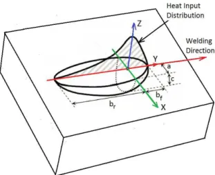
The initial condition is assumed with the workpiece setup to a given temperature and composition. For each time step, the geometry is actualized after metal deposition and moving heat source according to the assumed welding speed. For the boundary conditions, the effects of convective and radiative luxes are considered, while the heat input supplied by the torch is modeled by the power distribution given by the well-known moving Goldak’s double-ellipsoid heat source model26 (Figure1).
The model is a combination of two ellipses: one in the front quadrant of the heat source and the other in the rear quadrant. Equations 2 and 3 show the volumetric heat lux distributions inside the front and rear quadrant of the heat source, respectively. The model is deined as a function of position and time together with a number of parameters that affect the heat lux magnitude and distribution26.
(
, ,)
2 2 r y x z 3 3 3 b 2 a c r r r 6 3 f Qq x y z e e e
ab cπ π
−
− −
= (2)
(
, ,)
2 2
f
y
x 3 z
3 3
b
f a 2 c
f
f
6 3 f Q
q x y z e e e
ab cπ π
− − −
= (3)
Table 1. Chemical composition of the steel investigated (% wt.)16
C Si Mn Cr Cu Mo Ni
0.35 0.23 0.65 1.11 0.18 0.05 0.23
The heat input rate Q=hVI is determined by welding operational parameters current (I), voltage (V) and thermal eficiency h respectively. The factors ff and fr denote the fraction of the heat deposited in the front and rear quadrant respectively, which are setup to attain the restriction ff + fr = 2. The a,bf, c and br, are source constant parameters that deine the size and shape of the ellipses and, therefore, the heat source distribution. These parameters were estimated from the models for determination of the dimensions of a weld pool proposed by Wahab and Painter27 and may be
found in Table 2 together with the respective investigated welding parameters in this study, while the factors ff and fr
were deined as 0.6 and 1.4 respectively. Thickness and preheating effects on the welding region for the investigated steel were also carried out in order to evaluate the response of the present model when applied to more general cases. Further informations on the procedures adopted in this study are also available in table 2.
The cooling boundary conditions between the workpiece and environment by means of convection and radiation are calculated by Equations 4 and 5, respectively.
(
)
c 0
q =h T−T (4)
( ) ( 4 4)
r T 0
q =e sT −T (5)
where T0 (250 C) is the room temperature, e(T) is the emissivity
as a function of temperature, s( .5 67 x10−8 W m. −2.K−4) is the Stefan-Boltzmann constant and h(15W m. −2.K−4) is the natural convective heat coeficient assumed in this
study. The temperature dependency of emissivity for low carbon steels was investigated by Paloposki and Liedgust22, but limited for a narrow range of temperature
(up to 700 oC). The available data22 can be fitted as
shown in Equation 6. However, a common approach is to assume constant emissivity during welding simulations when Equations 2 and 3 are used to dynamically impose the volumetric heat source due to the welding arc, where the heat source parameters includes the net heat transferred to the workpiece at high temperatures5-13,17-19.
In this model, the Equation 6, obtained by regression of the data presented by Paloposki and Liedgust22, is used
for imposing the radiative cooling boundary conditions additionally to the double ellipsoid heat lux. Equation 6 predicts constant emissivity for temperature below 300 oC and above 750 oC. This behavior is due to the
range of measured data for low-alloyed steels, which is assumed to have similar behavior to the steel considered in this study. A clear shortcoming of this approach is that effects related to the surface parameters and environment temperature and composition are not considered and assumed negligible during the cooling by radiation and natural convection5-13,17-19. These shortcomings are usually
overcame by adjusting the heat source parameters, shown in Table 2, which is dominant for the high temperature region (above 750 oC), meanwhile, the radiation cooling effects for
low temperature (below 200 oC ) are negligible compared
with the convection contribution. Therefore, this approach has been widely used in welding simulation28-31.
( )T MAX 0 2 MIN 0 65
(
. ,(
. , ( .0 0016 T 0 7468. ))
)
e = − (6)
2.3. Thermophysical properties
The material properties were considered as temperature and composition dependent4,20,24,25. The heat capacity and
thermal conductivity are presented in Figures 2 and 3 respectively. Due to small variation of the density with temperature, this property was set as 7850kg m. −3. The thermal conductivity and speciic heat for individual phases reported in the literature depend of the authors, although follows similar trends4-21,24-33. The reason for such lack is due to
the possibility of different features of the phases formed depending on the thermal history. This paper uses a common approach assuming that the material obeys to a mixture rule pondered by the local volume fraction of each phase and for all thermophysical properties, which includes the transformations that the material undergoes during heating and cooling4-13,24-33.. Equations 7 an 8 are used to evaluate
the thermophysical properties dynamically during the phase
Figure 1 - Schematic model parameters for double-ellipsoid heat
source26.
Table 2. Welding and double-ellipsoid model parameters
Arc voltage (Volt)
Welding current (Amp)
Welding speed (mms-1)
Material Thickness (mm)
Heat input (kJ mm-1)
Double-ellipsoid model parameters (mm)
30 200 12 10 0.5 a= 4; bf=4; c= 2.5; br=16
30 200 12 10* 0.5 a = 4; bf=4; c=2.5; br= 16
30 200 2 10 3.0 a =9.5; bf= 9.5; c= 5; br= 38
30 200 2 25 3.0 a =9.5; bf= 9.5; c= 5; br= 38
transformations evolution which takes into account the mixture rule based on individual phase properties and volume fractions (xi). The equations 7 and 8 are used to estimate the heat capacity
(
Cp( )T x,)
and the thermal conductivity( )
k( )T x,for the low alloy steel used in this study. The temperature dependencies of heat capacity and thermal conductivities for
individual phases are taken from the correlations presented in Figures 2 and 3, respectively.
(T x, ) i i( ) i
Cp =∑x Cp T (7)
(T x, ) i i( ) i
k =∑x k T (8)
Figure 2 - Temperature-dependent of speciic heat for the investigated steel with individual phases during welding considered in this
model4,24,25.
2.4. Phase transformations
A phenomenological kinetic model based on the austenite diffusional transformation during cooling after austenitization of low-alloy hypoeutectoid steels was used for numerically to simulate the transformations from austenite into ferrite, pearlite and bainite simultaneously. In this section will be presented some features of the model. A more detailed description concerning to its formulation can be found in elsewhere16. Thus, the base of the extended version of the
multiphase diffusional transformation model of Avrami-type is represented by the Equation 9.
[
]
( i)i
1 1 m
1 m
i i
i i i i
i i
dy Y
m B Y y Ln
dt Y y
−
= − −
(9)
The temperature-dependent parameters Bi and mi are estimated from the TTT diagram for the investigated steel from the Equations 10 and 11.
( )
. ln i f s 6 1273 m T t t = (10)( )
. ( ) ii m T
s 0 01005 B T
t
= (11)
where ts and tf are the times correspondent to 1 and 99% of transformation, respectively.
Due to its importance during the austenite diffusional decomposition process, the austenitic grain growth was predicted by the temperature-dependent kinetic equation (Equation 12).
( )
A A n 1 A K T dDdt =n D − (12)
where,
( )
exp(
A)
A A
E
K T k
R T 273
= − +
(13)
In order to take into account the effect of austenitic grain size in the model, the Bi parameter in Equation 9 is deined as (14)
(
,)
( )
i
ref
i i i
D
B B T D B T
D e
= =
(14)
In Equations 12 to 14, kA was assumed as 6,087x107, n
A
was assumed as 2,44, EA is the activation energy for the growth process (317 kJ mol-1)16,21, R is the universal gas constant
(8,314 kJ K-1 mol-1), D
0 is the initial grain diameter at Ac3 temperature (0.00794 mm)16, B
i (T) parameter is obtained
from the isothermal diagram of the investigated steel by means of Equation 11, Dref corresponds to the reference grain diameter (0.0159 mm)16, e
i are positive constants varying
between 0.6 and 1.3 and depends upon the transformation type, i.e., ferrite, pearlite or bainite16.
After some modiications in order to take into account the coupling effects among the individual phase transformation
process, the multiphase model has its inal form represented by the coupled system of the differential Equations 15 to 19.
[
]
( 1)(
)
1
1 1 m
1 m Fe
1
1 1 Fe 1 Fe 1
Fe 1
Y dy
m K Y y Ln H Y y
dt Y y
−
= − − −
(15)
[
]
( 2)(
)
2
1 1 m
1 m Pe
2
2 2 Pe 2 Pe 2
Pe 2 Y dy
m K Y y Ln H Y y
dt Y y
−
= − − −
(16)
[ ] ( 3) ( )
3
1 1 m 1 m
3 Ba
3 3 Ba 1 3 Ba 3
Ba 1 3
dy Y
m K Y y y Ln H Y y
dt Y y y
−
= − − − − −
(17)
[
]
( )(
)
4 4 1 m 44 4 Ba 1 2 3 4
1 1 m
Ba 1 2 3
Ba 4
Ba 2 3 4
dy
m K Y y y y y
dt
Y y y y
Ln H Y y
Y y y y
− = − − − − − − − − − − − (18)
( )
a A n 1 A K T dDdt =n D − (19)
where y1, y2, y3 and y4 correspond to the products from austenite transformation, namely, ferrite, pearlite, upper and lower bainite, respectively; H (x) is the Heaviside function (in order to take into account the irreversibility of process);
m1, m2, m3 and m4 are parameters temperature-dependent obtained from the isothermal diagram of the investigated steel using Equation 10; YFe, YPe and YBa correspond to maximum volume fractions of ferrite, pearlite and bainite (Figure 4); K1, K2, K3 and K4 are functions deined by
Equation 20.
(
,)
( )
i
ref
i i i
D
K K T D B T
D e
= =
(20)
Meanwhile, the volume fraction of martensite was calculated using a novel model proposed by Lee and Van Tyne32 (Equation 21), which has been based on the well-known
Koistinen-Marburger model. Koistinen-Marburger model has been optimized by means of the introduction of two
Figure 4 - Estimated maximum volume fractions of ferrite, pearlite
parameters, KLV and nLV, which can be adjusted to take into account the several effects of the steel composition on the kinetic.
(
)
exp nLV
m LV s
V = −1 −K M −T (21)
where Vm is the volume fraction of martensite; T is the absolute temperature; Ms is the martensite start temperature and,
-
( )
1 . . . . .LV
K K− =0 0231 0 0105C− −0 0017 Ni 0 0074Cr+ −0 0193Mo (22)
- nLV=1 4304 1 1836C. − . +0 7527C. 2−0 0258 Ni 0 0739Cr. − . +0 3108Mo. (23)
2.5. Hardness
The hardness distribution at the HAZ of investigated steel was calculated by using the rule of mixtures (Equation 24).
(
)
v M M B B F P F P
H =X Hv +X Hv + X +X Hv + (24)
where Hv is the hardness (Vickers); XM, XB, XF and XP are the volume fractions of martensite, bainite, ferrite and pearlite, respectively; HvM, HvB and HvF+P are the hardness of martensite, bainite and the mixture of ferrite and pearlite, respectively.
For the calculating of HvM, HvB and HvF+P were used the formulae developed by Maynier et al.33 (Equations 25 to 27),
which take into account the steel composition and the cooling rate.
log M
Hv =127+949C+27 Si+11Mn+8 Ni+16Cr+21 Vr (25)
B
Hv = −323 185C+ +330Si+153Mn 65Ni+ +144Cr+191Mo+
(
89 53C 55Si 22Mn 10 Ni 20Cr 33Mo)
logVr+ + − − − − − (26)
. F P
Hv + =42+223C+53Si+30Mn 12 6 Ni 7Cr+ + +19Mo+
(
10 19Si 4 Ni 8Cr 130V)
logVr+ − + + + (27)
where Vr is the cooling rate at 700oC in °C.h–1.
At this point, is convenient to summarizes and point out the main features of the FVM computational code considered in this work and their shortcomings. Firstly, it is important to emphasize that the FVM computational code is able to handle complex geometries and non-linear temperature dependence on both boundary conditions and thermophysical properties, which are very important for practical applications. The main shortcomings, however, are related to the accuracy of the available data for thermophysical properties for the complete range of phase compositions developed by the steels during welding. However, the FVM computational code has been successfully applied and veriied for different materials and welding conditions and has been continuously updated for new applications and studies17-19. Another feature is that the
FVM computational code is an open source code, which can be updated using newly available data for properties and kinetic equations.
3. Results and Discussion
3.1. Thermal features
The numerical model for thermal analysis during welding, based in the mentioned FVM computational code, has been previously validated for the temperature ield predictions and previously published17-19 and new features incorporated in this
study. In order to demonstrate the accuracy of the prediction model, the Figures 5 (a) and (b) present a comparison between the calculated and measured values for temperature and welding zones in the plate. The temperature acquisition using thermocouples shows good agreement with the calculated results for a steel whose thermophysical and metallurgical features are quite representative of the steel investigated in this study, as shown in Figure 5 (a). As can be observed in Figure 5 (a), close agreement for the measured and calculated thermal history was obtained, allowing the applicability of the model for temperature predictions and welding zone (see Figure 5 (b)) and, accordingly, in providing of reliable data for the calculations of phase volume fractions.
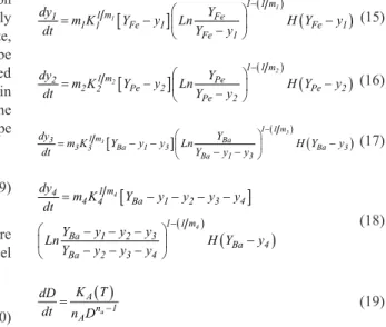
Figure 6 shows the results for three dimensional transient temperature distributions for the plates with different heat input and thickness. The results are shown for times that correspond to the temperature distribution on the plates when the welding heat source had already travelled an identical distance along of the different workpieces in each welding condition considered in this study (see Table 2). Thus, the corresponding welding times are 11.7 and 70 s for the heat inputs evaluated in this study, i.e., 0.5 and 3.0 kJ mm-1,
respectively.
Figure 5 - (a) Comparison for temperature evolution measured by thermocouples located at the bottom and centerline of the weldment and model predictions: Thermocouple (T1) and Thermocouple (T2) at 60 and 120 mm from origin of welding respectively and (b) Numerical and experimental comparison for the fusion zone (FZ) and heat affected zone (HAZ) in a transversal section located at 60 mm in the welding direction. Steel: 0.38%C, 0.96%Mn, 0.22%Si, 0.016%Cu, 0.12%Ni, 0.028%Cr, 0.03%Mo. Plate dimensions 10 x 60 x 220 mm. Heat input 1.5 kJ mm-1.
Figure 6 - Three dimensional transient temperature distribution during welding: (a) 0.5 kJ mm-1 and 10 mm thick (after 11.7 s); (b) 0.5 kJ mm-1
Figure 7 - Thermal proile in transversal sections of the plates: (a) 0.5 kJ mm-1 and 10 mm thick (after 9.2 s); (b) 0.5 kJ mm-1 and 10 mm
thick plus preheating (after 9.2 s); (c) 3 kJ mm-1 and 25 mm thick (after 55 s) and (d) 3 kJ mm-1 and 10 mm thick (after 55 s)
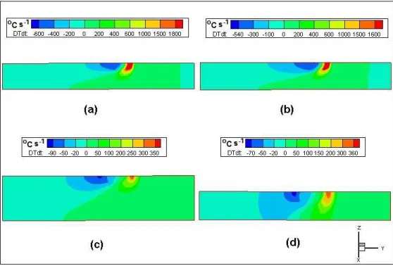
Figure 8 - Cooling and heating rates (oC s-1): (a) 0.5 kJ mm-1 and 10 mm thick (after 10.8 s); (b) 0.5 kJ mm-1 and 10 mm thick plus
Figure 8 shows the proile and the intensity of the cooling and heating rates acting along of the workpieces in a plane corresponding to its centerline at the welding direction. The welding times corresponding to the location of the heat source are 10.8 and 55.4 s for the heat inputs evaluated in this study, i.e., 0.5 and 3.0 kJ mm-1 respectively
(see table 2).
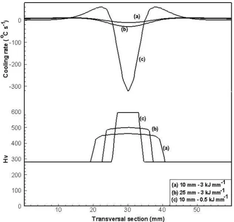
The preheating effect has resulted in lower cooling rates as can be seen in Figures 8(a) and (b) while keeping unchanged both the workpiece thickness and the heat input. As previously mentioned, higher thermal gradients are observed when thickness increases and greater cooling rates are reached accordingly. This behavior can be conirmed by comparing the Figures 8(c) and (d). In this case, only the workpiece thickness has changed. Figures 8(a) and (d) also allow a direct comparison from the inluence of heat input on the cooling rates when the workpiece thickness is kept unchanged and no preheating has been used, i.e., it can be observed that very lower cooling rate were reached when higher heat input was used. Figure 9 could complement the interpretation of these results.
Figure 9 shows the thermal cycles located at the HAZ where the peak temperature has reached about 1100oC in each
welding condition investigated (see Table 2). Furthermore, it is possible to notice the effects of variables such as preheating temperature and workpiece thickness on the cooling rates, which is in accordance with previous the discussions.
3.2. Phase transformations and grain growth
Figure 10 corresponds to the CCT diagram for the steel evaluated16 where are also plotted some calculated cooling
curves considering each investigated welding condition in this study (see Table 2). The cooling curves have started from a local at the HAZ where the peak temperature has reached about 1100oC, with the volume fraction of the constituents
and the hardness indicated in Figure 10 calculated using the mathematical formulation presented in this study.
Figures 11 and 12 present more comprehensive results depicting the HAZ and the resultant microstructure.
The results are shown for a speciic plane on the transversal section of the plates after cooling of weldment to room temperature. Furthermore, the boundaries between FZ and HAZ have been outlined in order to distinguish both weld regions, since the HAZ is the focus of this study. The only constituents predicted to occur at the HAZ using the numerical simulation were martensite and bainite. Indeed, a more comprehensive analysis based on that presented in Figure 10 can be carried out in order to correlate the different cooling rates locally reached within the HAZ with the microstructures predicted by the CCT diagram, which support both qualitatively and quantitatively the results shown in Figures 11 and 12.
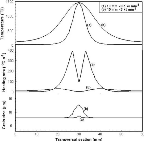
Figure 13 shows the inal grain size at the HAZ as consequence of thermal evolution during the welding taking into account the variables adopted in this study, whereas Figure 14 shows the effects of heating rate on the grain growth when comparing two different heat input and identical workpiece thickness. Heating rates in Figure 14 were calculated along transversal section of the workpiece referring to temperature of 1500oC, i.e., immediately below
of the FZ. Due to the comparatively shorter time exposed to elevated temperatures, the inal grain size was signiicantly lower when higher heating rates were reached, i.e., with decreasing heat input.
3.3. Hardness
Figure 15 shows the inal hardness distribution at the HAZ. Boundaries between FZ and HAZ have been again outlined by the same reasons previously mentioned. Calculated hardness values are compatible with those expected for the resultant microstructure and with those predicted by the CCT diagram of the steel investigated (see Figures 10 to 12).
Effects from the cooling rates caused by different welding conditions on the hardness proile along the transversal plane to the workpiece and crossing the HAZ can be seen in Figure 16. Accordingly, greater hardness levels were comparatively obtained with increasing cooling rates since it favors the formation of harder constituents as the martensite.
Figure 11 - Martensite distribution: (a) 0.5 kJ mm-1 (10 mm); (b) 0.5 kJ mm-1 (10 mm with preheating); (c) 3 kJ mm-1 (25 mm) and
(d) 3 kJ mm-1 (10 mm)
Figure 12 - Bainite distribution: (a) 0.5 kJ mm-1 (10 mm); (b) 0.5 kJ mm-1 (10 mm with preheating); (c) 3 kJ mm-1 (25 mm) and
Figure 13 - Final grain size at the HAZ: (a) 0.5 kJ mm-1 (10 mm); (b) 0.5 kJ mm-1 (10 mm with preheating); (c) 3 kJ mm-1 (25 mm) and
(d) 3 kJ mm-1 (10 mm)
Figure 15 - Final hardness distribution at the HAZ: (a) 0.5 kJ mm-1 (10 mm); (b) 0.5 kJ mm-1 (10 mm with preheating); (c) 3 kJ mm-1
(25 mm) and (d) 3 kJ mm-1 (10 mm)
4. Conclusions
In this study, a phenomenological model to predict the multiphase diffusional decomposition of the austenite during continuous cooling was implemented in a developed FVM computational code and applied for numerically to simulate the microstructure in the HAZ of a low-alloy hypoeutectoid steel. Thus, the results are summarized below.
a) The used methodology was able of satisfactorily to predict the phase transformations and the hardness distribution at the HAZ of the steel investigated. For this purpose, it was necessary to predict the temperature ield coupled dynamically with the welding evolution and the material thermophysical properties, together with the kinetics model for phase transformations and the model for hardness prediction.
b) Different welding conditions were simulated in order to evaluate the effectiveness of the methodology employed. Heat input, workpiece
thickness and preheating temperature were some of the investigated welding variables, which showed to play a fundamental effect on the thermal history from welding and, accordingly, on the resultant microstructure and the hardness distribution at the HAZ.
c) Grain growth at the HAZ showed be dependent on the heating rate, i.e., larger grain size was noticed to occur when lower heating rates were reached, i.e., with increasing heat input.
d) Elevated cooling rates have contributed for attaining higher hardness values in the HAZ, since it has favored the formation of harder constituents as the martensite.
Acknowledgements
This work was partially suported by CNPq, FINEP, FAPERJ and CAPES.
References
1. Grong Ø, Shercliff HR. Microstructural modelling in metals processing. Progress in Materials Science. 2002;47(2):163-282. doi:10.1016/S0079-6425(00)00004-9
2. Payares-Asprino C, Katsumoto H, Liu S. Effect of martensite start and finish temperature on residual stress development in structural steel welds. Welding Research. 2008;8:279S-289S. https://app.aws.org/wj/supplement/wj1108-279.pdf
3. Ju JB, Lee JS, Jang JI, Kim WS, Kwon D. Determination of welding residual stress distribution in API X65 pipeline using a modified magnetic Barkhausen noise method. International Journal of Pressure Vessels and Piping. 2003;80(9):641–646.
4. Zacharia T, Vitek JM, Goldak JA, DebyRoy TA, Rappaz M, Badeshia HK. Modeling fundamentals phenomena in welds. Modelling Simulation Materials Science Engineering. 1995;3:265-288.
5. Deng D. FEM prediction of welding residual stress and distortion in carbon steel considering phase transformation effects. Materials and Design. 2009;30:359–366.
6. Deng D, Murakawa H. Finite element analysis of temperature field, microstructure and residual stress in multi-pass butt-welded 2.25Cr–1Mo steel pipes. Computational Materials Science. 2008;43:681–695. DOI: 10.1016/j.commatsci.2008.01.025
7. Chen B, Flewitt PE, Smith DJ. Microstructural sensitivity of 316H austenitic stainless steel: Residual stress relaxation and grain boundary fracture. Materials Science and Engineering A. 2010;527:7387-7399. DOI: 10.1016/j.msea.2010.08.010
8. Heinze C, Schwenk C, Rethmeier M. Numerical calculation of residual stress development of multi-pass gas metal arc welding under high restraint conditions. Materials and Design. 2012;35(1):201–209. DOI: 10.1016/j.matdes.2011.09.021
9. Heinze C, Schwenk C, Rethmeier M. Numerical calculation of residual stress development of multi-pass gas metal arc welding. Journal of Constructional Steel Research. 2012;72:12–19. DOI: 10.1016/j.jcsr.2011.08.011
10. Chin-Hyung L, Kyong-Ho C. Prediction of residual stresses in high strength carbon steel pipe weld considering
solid-state phase transformation effects. Computers and Structures. 2011;89:256–265.
11. Deng D, Murakawa H. Prediction of welding residual stress in multi-pass butt-welded modified 9Cr–1Mo steel pipe considering phase transformation effects. Computational Materials Science. 2006;37(3):209–219. DOI: 10.1016/j.commatsci.2005.06.010
12. Thibault D, Bocher P, Thomas M. Residual stress and microstructure in welds of 13%Cr–4%Ni martensitic stainless steel. Journal of Materials Processing Technology. 2009; 209:2195–2202.
13. Francis JA, Bhadeshia HK, Withers PJ. Welding residual stresses in ferritic power plant steels. Materials Science and Technology. 2007;23(9):1009-1020.
14. Avrami MJ. Kinetics of phase change, I: General theory. Journal of Chemical Physics. 1939;7(12):1103–1112.
15. Cahn JW. Transformation kinetics during continuous cooling. Acta Metallurgica. 1956;4: 572-575. doi:10.1016/0001-6160(56)90158-4
16. Reti T, Fried Z, Felde I. Computer simulation of steel quenching process using a multi-phase transformation model. Computational Materials Science. 2001;22(3):261-278. DOI: http://dx.doi. org/10.1016/S0927-0256(01)00240-3
17. Xavier CR, Delgado Jr HG, Castro JA. An experimental and numerical approach for the welding effects on the duplex stainless steel microstructure. Materials Research. 2015; 18(3):489-502. http://dx.doi.org/10.1590/1516-1439.302014
18. Xavier CR, Delgado Junior HG, Castro JA. Numerical evaluation of the weldability of the low alloy ferritic steels T/P23 and T/P24. Materials Research. 2011;14(1):73-90. http://dx.doi. org/10.1590/S1516-14392011005000019
19. Xavier CR, Campos MF, Castro JA. Numerical method applied to duplex stainless steel. Ironmaking and Steelmaking. 2013;40(6):420-429. DOI:10.1179/1743281212Y.0000000065
20. Seok-Jae L, Pavlina EJ, Van Tyne CJ. Kinetics modeling of austenite decomposition for an end-quenched 1045 steel. Materials Science and Engineering A. 2010;527:3186-3194.
Handbook: Heat treating. Illinois: The Materials Information Company; 1991. p: 638-656. (ASM Handbook, 4)
22. Paloposki T, Liedgust L. Steel emissivity at high temperatures. VTT Research Notes. 2005;2229:1-81.
23. Jalaal M, Ghasemi E, Gani DD, Bararnia H, Soleimani S, Nejad MG, et al. Effect of temperature dependency of surface emissivity on heat transfer using the parameterized perturbation method. Thermal Science. 2011;15:S123-125. doi:10.2298/ TSCI11S1123J
24. Babu K, Prasanna Kumar TS. Comparison of austenite decomposition models during finite element simulation of water quenching and air cooling of AISI 4140 steels. Metallurgical and Materials Transactions B. 2014;45(4):1530-1544. DOI 10.1007/s11663-014-0069-0
25. Miettinen J, Lourenkilpi S. Calculation of thermophysical properties of carbon and low alloyed steels for modeling of solidification processes. Metallurgical and Materials Transactions B. 1994;25(6):909-916. DOI 10.1007/BF02662773
26. Goldak J, Chakravarti A, Bibby M. A new finite element model for welding heat sources. Metallurgical Transactions B. 1984;15(2): 299-305. DOI 10.1007/BF02667333
27. Wahab MA, Painter MJ. Numerical models of gas metal arc welds using experimentally determined weld pool shapes as the representation of the welding heat source. International Journal of Pressure Vessels and Piping. 1997;73(2):153-159. doi:10.1016/S0308-0161(97)00049-5
28. Harinadh V, Suresh A, Ramesh KB. Welding process simulation model for temperature and residual stress analysis. Procedia Materials Science. 2014;6:1539-1546.
29. Islam M, Buijk A, Rais-Rohani M, Motoyama K. Simulation-based numerical optimization of arc welding process for reduced distortion in welded structures. Finite Elements in Analysis and Design. 2014; 84: 54-64. http://www.mscsoftware.com/sites/ default/files/2014.1_Simulation_based_numerical_optimization_ of_arc_welding_process_for_reduced_distortion_in_welded_ structures.pdf
30. Ashok KK, Satish G, Lakshmi NV, Srinivasa RN. Development of mathematical model on gas tungsten arc welding process parameters. International Journal of Engineering Research and Technology. 2013;2:185-193.
31. Cho D, Song W, Cho M, Na S. Analysis of submerged arc welding-process by three dimensional computational fluid dynamics simulations. Journal of Materials Processing Technology. 2013;213:2278-2291.
32. Seok-Jae L, Van Tyne CJ. A kinetics model for martensite transformation in plain carbon and low-alloyed steels. Metallurgical and Materials Transactions A. 2012;43(2):422-427. DOI 10.1007/s11661-011-0872-z