Repositório Institucional UFC: On the efficient design of extreme learning machines using intrinsic plasticity and evolutionary computation approaches

(1)

CENTRO DE TECNOLOGIA

DEPARTAMENTO DE ENGENHARIA DE TELEINFORM ´ATICA

PROGRAMA DE P ÓS-GRADUA ¸C ÃO EM ENGENHARIA DE TELEINFORM ÁTICA

ANANDA LIMA FREIRE

ON THE EFFICIENT DESIGN OF EXTREME LEARNING MACHINES USING INTRINSIC PLASTICITY AND EVOLUTIONARY

COMPUTATION APPROACHES

(2)

ON THE EFFICIENT DESIGN OF EXTREME LEARNING MACHINES USING INTRINSIC PLASTICITY AND EVOLUTIONARY COMPUTATION APPROACHES

Tese apresentada ao Programa de Pós-Gradua¸cão em Engenharia de Teleinformática do Centro de Tecnologia da Universidade Federal do Ceará, como requisito parcial à obten¸cão do t´ıtulo de doutor em Engenharia de Teleinformática. Área de Concentra¸cão: Sinais e sistemas

Orientador: Prof. Dr. Guilherme de Alencar Barreto

(3)

Biblioteca Universitária

Gerada automaticamente pelo módulo Catalog, mediante os dados fornecidos pelo(a) autor(a)

F933o Freire, Ananda Lima.

On the Efficient Design of Extreme Learning Machines Using Intrinsic Plasticity and Evolutionary Computation Approaches / Ananda Lima Freire. – 2015.

222 f. : il. color.

Tese (doutorado) – Universidade Federal do Ceará, Centro de Tecnologia, Programa de Pós-Graduação em Engenharia de Teleinformática, Fortaleza, 2015.

Orientação: Prof. Dr. Guilherme de Alencar Barreto.

1. Máquina de Aprendizado Extremo. 2. Robustez a Outliers. 3. Metaheurísticas. I. Título.

(4)

ON THE EFFICIENT DESIGN OF EXTREME LEARNING MACHINES USING INTRINSIC PLASTICITY AND EVOLUTIONARY COMPUTATION APPROACHES

Thesis presented to the Graduate Pro-gram in Teleinformatics Engineering of the Federal University of Cear´a in partial fulﬁllment of the requirements for the degree of Doctor in the area of Teleinformatics Engineering. Concen-tration Area of Study: Signals and Systems

Date Approved: February 10, 2015

EXAMINING COMMITTEE

Prof. Dr. Guilherme de Alencar Barreto (Committee Chair / Advisor) Federal University of Cear´a (UFC)

Prof. Dr. George André Pereira Thé Federal University of Ceará (UFC)

Prof. Dr. Marcos Jos´e Negreiros Gomes State University of Cear´a (UECE)

(5)

(6)

First and foremost, I want to thank my beloved ones, Odete and Victor, for their love and support through this journey. Thank you for giving me the strength to deal with the distresses of this path and helping me to chase my dreams.

I would like to sincerely thank my advisor, Prof. Dr. Guilherme Barreto, for his guidance, patient encouragement and conﬁdence in me throughout this study, and especially his unhesitating support in a dark and personal moment I had been through. I would also like to thank Prof. Dr. Jochen Steil for accepting me to work at CoR-Lab under his supervision. I learned a lot from that experience, not only in a professional sphere but also as a person.

To the Professors Dr. George Th´e, Dr. Marcos Gomes, Dr. Felipe Fran¸ca and Dr. Frederico Guimar˜aes, thank you for your time and valuable contributions to the improvement of this work.

To my colleagues, both in UFC and in CoR-Lab, thank you all for making the work places such pleasant environments and for always being available for discussions.

To CAPES and the DAAD/CNPq scholarship program, thank you for the ﬁnancial support.

To NUTEC and CENTAURO for providing their facilities.

I would also like to thank the secretaries and Coordination Departments of both UFC and Universit¨at Bielefeld for their support.

(7)

A rede Máquina de Aprendizado Extremo (Extreme Learning Machine - ELM) tornou-se uma arquitetura neural bastante popular devido a sua propriedade de aproximadora universal de fun¸cões e ao rápido treinamento, dado pela sele¸cão aleatória dos pesos e limiares dos neurônios ocultos. Apesar de sua boa capacidade de generaliza¸cão, há ainda desafios consideráveis a superar. Um deles refere-se ao clássico problema de se determinar o número de neurônios ocultos, o que influencia na capacidade de aprendizagem do modelo, levando a um sobreajustamento, se esse número for muito grande, ou a um subajustamento, caso contrário. Outro desafio está relacionado à sele¸cão aleatória dos pesos da camada oculta, que pode produzir uma matriz de ativa¸cões mal-condicionada, dificultando sensivelmente a solu¸cão do sistema linear constru´ıdo para treinar os pesos da camada de sa´ıda. Tal situa¸cão leva a solu¸cões com normas muito elevadas e, consequentemente, numericamente instáveis. Baseado nesses desafios, este trabalho oferece duas contribui¸cões orientadas a um projeto eficiente da rede ELM. A primeira, denominada R-ELM/BIP, combina a versão batch de um método de aprendizado recente chamado Plasticidade Intr´ınseca com a técnica de estima¸cão robusta conhecida como Estima¸cão M. Esta proposta fornece solu¸cão confiável na presen¸ca de outliers, juntamente com boa capacidade de generaliza¸cão e pesos de sa´ıda com normas reduzidas. A segunda contribui¸cão, denominada Adaptive Number of Hidden Neurons Approach (ANHNA), está orientada para a sele¸cão automática de um modelo de rede ELM usando metaheur´ısticas. A ideia subjacente consiste em definir uma codifica¸cão geral para o indiv´ıduo de uma popula¸cão que possa ser usada por diferentes metaheur´ısticas populacionais, tais como Evolu¸cão Diferencial e Enxame de Part´ıculas. A abordagem proposta permite que estas metaheur´ısticas produzam solu¸cões otimizadas para os vários parâmetros da rede ELM, incluindo o número de neurônios ocultos e as inclina¸cões e limiares das fun¸cões de ativa¸cão dos mesmos, sem perder a principal caracter´ıstica da rede ELM: o mapeamento aleatório do espa¸co da camada oculta. Avalia¸cões abrangentes das abordagens propostas são realizadas usando conjuntos de dados para regressão dispon´ıveis em repositórios públicos, bem como um novo conjunto de dados gerado para o aprendizado da coordena¸cão visuomotora de robôs humanoides.

(8)

The Extreme Learning Machine (ELM) has become a very popular neural network ar-chitecture due to its universal function approximation property and fast training, which is accomplished by setting randomly the hidden neurons’ weights and biases. Although it offers a good generalization performance with little time consumption, it also offers considerable challenges. One of them is related to the classical problem of defining the network size, which influences the ability to learn the model and will overfit if it is too large or underfit if it is too small. Another is related to the random selection of input-to-hidden-layer weights that may produce an ill-conditioned hidden input-to-hidden-layer output matrix, which derails the solution for the linear system used to train the output weights. This leads to a solution with a high norm that becomes very sensitive to any contamination present in the data. Based on these challenges, this work provides two contributions to the ELM network design principles. The first one, named R-ELM/BIP, combines the maximization of the hidden layer’s information transmission, through Batch Intrinsic Plasticity, with outlier-robust estimation of the output weights. This method generates a reliable solution in the presence of corrupted data with a good generalization capability and small output weight norms. The second method, named Adaptive Number of Hidden Neurons Approach (ANHNA), is defined as a general solution encoding that allows populational metaheuristics to evolve a close to optimal architecture for ELM networks combined with activation function’s parameter optimization, without losing the ELM’s main feature: the random mapping from input to hidden space. Comprehensive evaluations of the proposed approaches are performed using regression datasets available in public repositories, as well as using a new set of data generated for learning visuomotor coordination of humanoid robots.

(9)

Figure 1 – Extreme Learning Machine architecture. . . 36

Figure 2 – Scatter plot of Table 2 dataset. . . 47

Figure 3 – Regression with and without the USA sample. . . 47

Figure 4 – Diﬀerent objective functions ρ(ε)with k=1. . . 52

Figure 5 – Diﬀerent weight functions w(ε) with k=1. . . 53

Figure 6 – Regression without USA outlier. . . 54

Figure 7 – Regression with USA outlier. . . 55

Figure 8 – Architecture, connectivity matrix and binary string representation. . . 63

Figure 9 – ANHNA’s i-th chromosome representation. . . 65

Figure 10 – ANHNA’s i-th chromosome representation with regularization. . . 70

Figure 11 – ANHNA’s i-th chromosome representation for robust ELM networks. . 71

Figure 12 – Data separation in test and training samples. . . 77

Figure 13 – A 5-fold cross validation procedure. . . 77

Figure 14 – Flow chart of the experiments with robust ELM networks. . . 78

Figure 15 – Flow chart of the experiments with ANHNA. . . 79

Figure 16 – Testing RMSE of robust ELM networks (1s - iCub dataset). . . 84

Figure 17 – Testing RMSE of robust ELM networks (2s - iCub dataset). . . 84

Figure 18 – Number of hidden neurons of robust ELM networks (1s - iCub dataset). 85 Figure 19 – Number of hidden neurons of robust ELM networks (2s - iCub dataset). 85 Figure 20 – Testing RMSE of robust ELM networks (1s - Auto-MPG dataset). . . . 88

Figure 21 – Testing RMSE of robust ELM networks (2s - Auto-MPG dataset). . . . 88

Figure 22 – Number of hidden neurons of robust ELM networks (1s - Auto-MPG dataset). . . 89

Figure 23 – Number of hidden neurons of robust ELM networks (2s - Auto-MPG dataset). . . 89

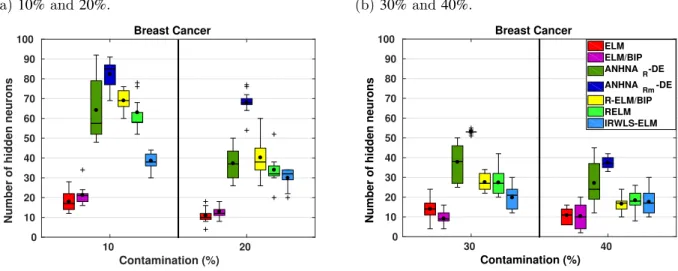
Figure 24 – Testing RMSE of robust ELM networks (1s - Breast Cancer dataset). . 92

Figure 25 – Testing RMSE of robust ELM networks (2s - Breast Cancer dataset). . 92

Figure 26 – Number of hidden neurons of robust ELM networks (1s - Breast Cancer dataset). . . 92

(10)

Figure 29 – Testing RMSE of robust ELM networks (2s - CPU dataset). . . 95

Figure 30 – Number of hidden neurons of robust ELM networks (1s - CPU dataset). 95 Figure 31 – Number of hidden neurons of robust ELM networks (1s - CPU dataset). 96 Figure 32 – Testing RMSE of robust ELM networks (1s - Servo dataset). . . 98

Figure 33 – Testing RMSE of robust ELM networks (2s - Servo dataset). . . 98

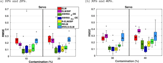
Figure 34 – Number of hidden neurons of robust ELM networks (1s - Servo dataset). 98 Figure 35 – Number of hidden neurons of robust ELM networks (2s - Servo dataset). 99 Figure 36 – ANHNA comparison with diﬀerent metaheuristics (Auto-MPG dataset). 105 Figure 37 – ANHNA comparison with diﬀerent metaheuristics (Bodyfat dataset). . 106

Figure 38 – ANHNA comparison with diﬀerent metaheuristics (Breast Cancer dataset).108 Figure 39 – ANHNA comparison with diﬀerent metaheuristics (CPU dataset). . . . 109

Figure 40 – ANHNA comparison with diﬀerent metaheuristics (iCub dataset). . . . 111

Figure 41 – ANHNA comparison with diﬀerent metaheuristics (Servo dataset). . . . 113

Figure 42 – PSO topologies. . . 136

Figure 43 – Setup for iCub’s dataset harvesting. . . 141

Figure 44 – ANHNA-DE’s variants for Auto-MPG dataset with DE. . . 156

Figure 45 – ANHNA-DE’s variants for Bodyfat dataset with DE. . . 157

Figure 46 – ANHNA-DE’s variants for Breast Cancer dataset with DE. . . 158

Figure 47 – ANHNA-DE’s variants for CPU dataset with DE. . . 159

Figure 48 – ANHNA-DE’s variants for iCub dataset with DE. . . 160

Figure 49 – ANHNA-DE’s variants for Servo dataset with DE. . . 161

Figure 50 – ANHNA’s variants for Bodyfat dataset with PSOg. . . 162

Figure 51 – ANHNA’s variants for Breast Cancer dataset with PSOg. . . 163

Figure 52 – ANHNA’s variants for Bodyfat dataset with PSOl. . . 165

Figure 53 – ANHNA’s variants for Breast Cancer dataset with PSOl. . . 166

Figure 54 – ANHNA’s variants for Bodyfat dataset with SADE. . . 167

Figure 55 – ANHNA’s variants for Breast Cancer dataset with SADE. . . 168

Figure 56 – ANHNA-DERe convergence (1-4/10) for Auto-MPG dataset. . . 169

Figure 57 – ANHNA-DERe convergence (5-10/10) for Auto-MPG dataset. . . 170

Figure 58 – ANHNA-DERe convergence (1-6/10) for Bodyfat dataset. . . 171

(11)

Figure 61 – ANHNA-DERe convergence (3-10/10) for Breast Cancer dataset. . . 173

Figure 62 – ANHNA-DERe convergence (1-8/10) for CPU dataset. . . 174

Figure 63 – ANHNA-DERe convergence (9-10/10) for CPU dataset. . . 175

Figure 64 – ANHNA-DERe convergence (1-4/10) for iCub dataset. . . 175

Figure 65 – ANHNA-DERe convergence (5-10/10) for iCub dataset. . . 176

Figure 66 – ANHNA-DERe convergence (1-8/10) for Servo dataset. . . 177

Figure 67 – ANHNA-DERe convergence (9-10/10) for Servo dataset. . . 178

Figure 68 – ANHNAR-DE weight function choice for Auto-MPG (10%-1s) dataset. 179 Figure 69 – ANHNAR-DE error threshold evolution for Auto-MPG (10%-1s) dataset.179 Figure 70 – ANHNAR-DE weight function choice for Auto-MPG (20%-1s) dataset. 180 Figure 71 – ANHNAR-DE error threshold evolution for Auto-MPG (20%-1s) dataset.180 Figure 72 – ANHNAR-DE weight function choice for Auto-MPG (30%-1s) dataset. 180 Figure 73 – ANHNAR-DE error threshold evolution for Auto-MPG (30%-1s) dataset.181 Figure 74 – ANHNAR-DE weight function choice for Auto-MPG (40%-1s) dataset. 181 Figure 75 – ANHNAR-DE error threshold evolution for Auto-MPG (40%-1s) dataset.181 Figure 76 – ANHNAR-DE weight function choice for Auto-MPG (10%-2s) dataset. 182 Figure 77 – ANHNAR-DE error threshold evolution for Auto-MPG (10%-2s) dataset.182 Figure 78 – ANHNAR-DE weight function choice for Auto-MPG (20%-2s) dataset. 182 Figure 79 – ANHNAR-DE error threshold evolution for Auto-MPG (20%-2s) dataset.183 Figure 80 – ANHNAR-DE weight function choice for Auto-MPG (30%-2s) dataset. 183 Figure 81 – ANHNAR-DE error threshold evolution for Auto-MPG (30%-2s) dataset.183 Figure 82 – ANHNAR-DE weight function choice for Auto-MPG (40%-2s) dataset. 184 Figure 83 – ANHNAR-DE error threshold evolution for Auto-MPG (40%-2s) dataset.184 Figure 84 – ANHNAR-DE weight function choice for Breast Cancer (10%-1s) dataset.184 Figure 85 – ANHNAR-DE error threshold evolution for Breast Cancer (10%-1s) dataset. . . 185

(12)

dataset. . . 186 Figure 90 – ANHNAR-DE weight function choice for Breast Cancer (40%-1s) dataset.186

Figure 91 – ANHNAR-DE error threshold evolution for Breast Cancer (40%-1s)

dataset. . . 189 Figure 100 – ANHNAR-DE weight function choice for CPU (10%-1s) dataset. . . 190

Figure 101 – ANHNAR-DE error threshold evolution for CPU (10%-1s) dataset. . . . 190

Figure 102 – ANHNAR-DE weight function choice for CPU (20%-1s) dataset. . . 190

(13)

Figure 116 – ANHNAR-DE weight function choice for Servo (10%-1s) dataset. . . 195

Figure 117 – ANHNAR-DE error threshold evolution for Servo (10%-1s) dataset. . . 195

Figure 132 – ANHNARm-DE weight function choice for Auto-MPG (10%-1s) dataset. 200

Figure 133 – ANHNARm-DE error threshold evolution for Auto-MPG (10%-1s) dataset.201

(14)

Figure 148 – ANHNARm-DE weight function choice for Breast Cancer (10%-1s) dataset.206

Figure 149 – ANHNARm-DE error threshold evolution for Breast Cancer (10%-1s)

dataset. . . 206 Figure 150 – ANHNARm-DE weight function choice for Breast Cancer (20%-1s) dataset.206

Figure 160 – ANHNARm-DE weight function choice for Breast Cancer (30%-2s) dataset.209

dataset. . . 210 Figure 161 – ANHNARm-DE error threshold evolution for Breast Cancer (30%-2s)

dataset. . . 211 Figure 164 – ANHNARm-DE weight function choice for CPU (10%-1s) dataset. . . . 211

Figure 165 – ANHNARm-DE error threshold evolution for CPU (10%-1s) dataset. . . 211

Figure 166 – ANHNARm-DE weight function choice for CPU (20%-1s) dataset. . . . 212

(15)

Figure 180 – ANHNARm-DE weight function choice for Servo (10%-1s) dataset. . . . 216

Figure 181 – ANHNARm-DE error threshold evolution for Servo (10%-1s) dataset. . . 217

(16)

Table 1 – Thesis time-line. . . 28

Table 2 – Cigarette consumption dataset. . . 46

Table 3 – Objective functions, weight functions and default thresholds. . . 51

Table 4 – Weight values for diﬀerent M-Estimators with Cigarette dataset. . . 55

Table 5 – Codiﬁcation for choosing the weight function. . . 71

Table 6 – Division of samples for each fold in cross validation. . . 80

Table 7 – Output weight euclidean norm (1s - iCub dataset). . . 87

Table 8 – Output weight euclidean norm (2s - iCub dataset). . . 87

Table 9 – Output weight euclidean norm (1s - Auto-MPG dataset). . . 90

Table 10 – Output weight euclidean norm (2s - Auto-MPG dataset). . . 91

Table 11 – Output weight euclidean norm (1s - Breast Cancer dataset). . . 93

Table 12 – Output weight euclidean norm (2s - Breast Cancer dataset). . . 94

Table 13 – Output weight euclidean norm (1s - CPU dataset). . . 96

Table 14 – Output weight euclidean norm (2s - CPU dataset). . . 97

Table 15 – Output weight euclidean norm (1s - Servo dataset). . . 99

Table 16 – Output weight euclidean norm (2s - Servo dataset). . . 100

Table 17 – Evaluation results of weight norms (Auto-MPG dataset). . . 103

Table 18 – Regularization parameters (Auto-MPG dataset). . . 103

Table 19 – Evaluation results of weight norms (Bodyfat dataset). . . 106

Table 20 – Regularization parameters (Bodyfat dataset). . . 107

Table 21 – Evaluation results of weight norms (Breast Cancer dataset). . . 107

Table 22 – Regularization parameters (Breast Cancer dataset). . . 107

Table 23 – Evaluation results of weight norms (CPU dataset). . . 110

Table 24 – Regularization parameters (CPU dataset). . . 110

Table 25 – Evaluation results of weight norms (iCub dataset). . . 110

Table 26 – Regularization parameters (iCub dataset). . . 111

Table 27 – Evaluation results of weight norms (Servo dataset). . . 112

Table 28 – Regularization parameters (Servo dataset). . . 112

Table 29 – Success memory. . . 133

(17)

Table 33 – Number of hidden neurons (2s) with iCub dataset. . . 144

Table 34 – Number of hidden neurons (1s) with Auto-MPG dataset. . . 145

Table 35 – Number of hidden neurons (2s) with Auto-MPG dataset. . . 146

Table 36 – Number of hidden neurons (1s) with Bodyfat dataset. . . 147

Table 37 – Number of hidden neurons (2s) with Bodyfat dataset. . . 148

Table 38 – Number of hidden neurons (1s) with Breast Cancer dataset. . . 149

Table 39 – Number of hidden neurons (2s) with Breast Cancer dataset. . . 150

Table 40 – Number of hidden neurons (1s) with CPU dataset. . . 151

Table 41 – Number of hidden neurons (2s) with CPU dataset. . . 152

Table 42 – Number of hidden neurons (1s) with Servo dataset. . . 153

Table 43 – Number of hidden neurons (2s) with Servo dataset. . . 154

Table 44 – ANHNA-DE’s comparison study of weight norm (Auto-MPG dataset). . 156

Table 45 – ANHNA-DE’s comparison study of weight norm (Bodyfat dataset). . . . 157

Table 46 – ANHNA-DE’s comparison study of weight norm (Breast Cancer dataset).158 Table 47 – ANHNA-DE’s comparison study of weight norm (CPU dataset). . . 159

Table 48 – ANHNA-DE’s comparison study of weight norm (iCub dataset). . . 160

Table 49 – ANHNA-DE’s comparison study of weight norm (Servo dataset). . . 161

Table 50 – ANHNA-PSOg’s comparison study of weight norm (Bodyfat dataset). . 163

Table 51 – ANHNA-PSOg’s comparison study of weight norm (Breast Cancer dataset).164 Table 52 – ANHNA-PSOl’s comparison study of weight norm (Bodyfat dataset). . 164

Table 53 – ANHNA-PSOl’s comparison study of weight norm (Breast Cancer dataset).165 Table 54 – ANHNA’s comparison study of weight norm (Bodyfat dataset). . . 166

(18)

Algorithm 1 – Extreme Learning Machine . . . 38

Algorithm 2 – Batch Intrinsic Plasticity . . . 43

Algorithm 3 – Iteratively Reweighted Least Squares . . . 50

Algorithm 4 – R-ELM/BIP . . . 58

Algorithm 5 – ANHNA-DE Pseudocode {Qmin,Qmax} . . . 68

Algorithm 6 – ANHNA-PSO Pseudocode {Qmin,Qmax} . . . 68

Algorithm 7 – ANHNAR-DE Pseudocode {Qmin,Qmax} . . . 73

Algorithm 8 – General DE Algorithm . . . 129

Algorithm 9 – General SaDE Algorithm (QIN et al., 2009) . . . 135

Algorithm 10 – gbest PSO . . . 138

(19)

ANHNA Adaptive Number of Hidden Neurons Approach

ANN Artiﬁcial Neural Network

BIP Batch Intrinsic Plasticity

Cor-Lab Research Institute of Cognition and Robotics

DE Diﬀerential Evolution

EANN Evolutionary Artiﬁcial Neural Networks

ECOD Extended Complete Orthogonal Decomposition

ELM Extreme Learning Machine

EI-ELM Enhanced Incremental Extreme Learning Machine EM-ELM Error Minimized Extreme Learning Machine

ESN Echo State Network

GA Genetic Algorithm

GO-ELM Genetically Optimized Extreme Learning Machine I-ELM Incremental Extreme Learning Machine

IP Intrinsic Plasticity

LMS Least Mean Square

LSM Liquid State Machines

MLP Multilayer Perceptron

OP-ELM Optimally Pruned Extreme Learning Machine

PSO Particle Swarm Optimization

RBF Radial Basis Function

RMSE Root Mean Square Error

(20)

β β

β ELM’s output weight vector

γ Parameter that controls greedness of the mutation operator

ν ν

νi Velocity of i-th PSO particle κ Condition number of a matrix

λ Regularization parameter

ψ Derivative of rho

ρ Weighting function for M-Estimators

σmax Largest eigenvalue of a matrix σmin Smallet eigenvalue of a matrix

τ Set of 3 bits that determines the weight function

υ Tunning constant for a weight function

a Slope parameter for sigmoid and hiperbolic tangent activation functions

b Bias

C Population set of a metaheuristic algorithm

c Individual or particle vector of a metaheuristic algorithm c′ Oﬀspring vector of a metaheuristic algorithm

cbest PSO’s global best position of all swarm

CR Crossover rate

CRmk Median value of crossover rate for a givenk strategy in SaDE algorithm

CRmemoryk Memory that stores the CR values of sucessful k-th strategy

D Desired output matrix

d Desired output vector

dn Dimension of a individual or particle vector

F Scaling factor

g Current generation for a given metaheuristic

(21)

LP Learning period

LS Least Squares

m ELM’s hidden layer weights

N Number of training samples

Pr Dimensionality of the search space

pk k-th Strategy probability

p ELM’s input pattern dimension

pl_k PSO’s k-th neighborhood best position

pi PSO’s previous personal best position of i-th particle

Qmax Maximum number of hidden neurons for ANHNA

Qmin Minimum number of hidden neurons for ANHNA

q Number of hidden neurons

N Normal distribution

ns_k Number of oﬀsprings generated with k-th strategy that successfuly passed to the next generation

n fk Number of oﬀsprings generated withk-th strategy that were discarded

nv Number of diﬀerences in a mutation operator

r ELM’s output layer dimension

Sk Success rate of the oﬀsprings by the k-th strategy

U Uniform distribution

U Input matrix

u Input vector

v Trial vector for DE and SaDE algorithms

(22)

1 INTRODUCTION . . . 23

1.1 General and specific objectives . . . 25

1.2 A word on the thesis’ chronology and development. . . 26

1.3 Scientific production . . . 29

1.4 Thesis structure . . . 31

2 THE EXTREME LEARNING MACHINE . . . 33

2.1 Random projections in the literature . . . 33

2.2 Introduction to ELM. . . 35

2.3 Issues and improvements for ELM . . . 38 2.3.1 Tikhonov’s regularization . . . 38 2.3.2 Architecture optimization . . . 40 2.3.3 Intrinsic plasticity . . . 41

2.4 Concluding remarks . . . 43

3 A ROBUST ELM/BIP . . . 45

3.1 Outliers influence . . . 46

3.2 Fundamentals of Maximum Likelihood Estimation . . . 48 3.2.1 Objective and Weighting Functions for M-Estimators . . . . 50 3.2.2 Numerical example . . . 54

3.3 Robustness in ELM networks . . . 55

3.4 R-ELM/BIP . . . 57

4 A NOVEL MODEL SELECTION APPROACH FOR THE ELM 59

4.1 Introduction to metaheuristics. . . 59

4.2 Related works . . . 61

4.3 Encoding schemes for architecture evolution . . . 63

4.4 The Adaptive Number of Hidden Neurons Approach . . . 65 4.4.1 Variants of ANHNA . . . 68

4.4.1.1 Using the condition number of H and the norm of the output weight vector 69 4.4.1.2 Using regularization . . . 70

4.4.2 ANHNA for robust regression . . . 71

(23)

5.1 Data treatment . . . 75 5.1.1 Outlier contamination. . . 75

5.2 Experiments . . . 76

5.3 Parameters . . . 80

6 PERFORMANCE ANALYSIS OF THE ROBUST ELM . . . 83

6.1 Comparison of robust ELM networks . . . 83 6.1.1 iCub dataset . . . 84 6.1.2 Auto-MPG dataset . . . 88 6.1.3 Breast Cancer dataset. . . 91 6.1.4 CPU dataset . . . 95 6.1.5 Servo dataset . . . 98

7 PERFORMANCE ANALYSIS OF THE ANHNA . . . 102

7.1 ANHNA’s comparative study . . . 103 7.1.1 Auto-MPG dataset . . . 103 7.1.2 Bodyfat dataset . . . 105 7.1.3 Breast Cancer dataset. . . 107 7.1.4 CPU dataset . . . 108 7.1.5 iCub dataset . . . 110 7.1.6 Servo dataset . . . 112

8 CONCLUSIONS AND FUTURE WORK . . . 114

8.1 Future Work . . . 117

BIBLIOGRAPHY . . . 118

APˆENDICES . . . 128

APPENDIX A – Evolutionary Algorithms . . . 128

APPENDIX B – Datasets . . . 140

APPENDIX C – Detailed Tables for Robust ELM . . . 143

APPENDIX D – Results of ANHNA’s variants . . . 155

APPENDIX E – ANHNA’s convergence . . . 169

(24)

1 INTRODUCTION

Among the different artificial neural network (ANN) architectures available, the single layer feedforward one (SLFN) is the most popular (HUANG et al., 2011). It is specially known by its universal approximation abilities (CAO et al., 2012). In particular, the Extreme Learning Machine (ELM) is attracting considerable attention from the Computational Intelligence community due to its fast training speed by randomly selecting the weights and biases of the hidden neurons. This singular feature allows the problem of estimating the output weights to be cast as a linear model, which is then analytically determined by finding a least-squares solution (HUANG et al., 2011).

However, there is no free lunch. Even though this network is capable of achieving a good generalization performance with little time consumption, it also offers considerable challenges. One of these issues is related to an inherited problem from standard SLFN: the definition of the number of hidden neurons. A small network may not provide a good performance due to its limited information processing which leads to a too simplistic model, while a large one may lead to overfitting and poor generalization. To correctly define the number of hidden neurons, the most common strategy is to resort to trial-and-error or exhaustive search strategies (YANG et al., 2012).

Another issue is related to the random nature of the input-to-hidden-layer weights (hidden weights, for short). This random combination often generates a set of non-optimal weights and biases, which results in an ill-conditioned matrix of hidden neurons’ activations H. Such situation makes the solution of the linear output system numerically unstable due to the very high norm of the resulting output weight vector and, hence, make the whole network very sensitive to data perturbation (e.g. outliers) (ZHAO

et al., 2011). Furthermore, as described in the work of Bartlett (1998), their size is more relevant for the generalization capability than the conﬁguration of the neural network itself.

(25)

to the conditioning of H matrix, as well as with outlier robustness by choosing estimation methods, other than the standard least-squares approach, which are capable of dealing with outliers.

Knowing that methods which control only the network size and the output weights are insuﬃcient in tunning the hidden neurons to a good regime, where the encoding is optimal (NEUMANN; STEIL, 2011), we took the Intrinsic Plasticity (IP) notion as inspiration to tackle the computational robustness problem. This biologically motivated mechanism was ﬁrst introduced by Triesch (2005) and consists in adapting the activation function’s parameters (slope and bias) to force the output of the hidden neurons to follow an exponential distribution (stochastically speaking). This maximizes the information transmission caused by the high entropy of this probability distribution. (NEUMANN; STEIL, 2011). Empirically, it also results in a more stable H matrix followed by a smaller norm of the output weights than the ones provided by the standard least-squares method.

Regarding outlier robustness, even though robust ANN is a subject of interest in Machine Learning, the study of this property with ELM network is still in its infancy (HORATA et al., 2013). Works such as Huynh, Won and Kim (2008), Barros and Barreto (2013), Horata, Chiewchanwattana and Sunat (2013) adopt an estimation method that is less sensitive to outliers than the ordinary least-squares estimation, known as M-estimation

(HUBER, 1964). However, Horata’s work is the only one that addresses both computational and outlier robustness problem.

Hence, one of the contributions of this work is a robust version of ELM network that incorporates both regularizing and outlier robustness features to ELM learning, by combining the optimization of the hidden layer output through a new method named Batch Intrinsic Plasticity (BIP) (NEUMANN; STEIL, 2011) with the M-estimation method.

Turning to the ﬁrst mentioned ELM’s challenge, to deal with its architecture design issue, we choose the use of population-based metaheuristics due to the complex task of ﬁnding suitable values for the number of hidden neurons and also to other learning parameters, such as the slopes and biases of the hidden activation functions. The use of evolutionary computation on ELM networks has been a quite popular subject. As examples, we mention works such as Zhu et al. (2005), Xu and Shu (2006), Silva et al.

(26)

these works are not designed to automatically determine the optimal number of hidden neurons. In other words, most of them predefine the number of hidden neurons and they usually concentrate the efforts on using those metaheuristics to find optimal values for the input-to-hidden layer weights. This approach, however, goes against the very nature of the ELM network, that is, to be an SLFN whose parameters of the input-to-hidden projection is specified randomly.

In order to propose an improved design for the ELM network following the Intrinsic Plasticity learning principles, we introduce a new encoding scheme for the solution vector of a given metaheuristic optimization algorithm that allows automatic estimation of the number of hidden neurons and their activation function parameter values. This scheme, namedAutomatic Number of Hidden Neurons Approach (ANHNA), is very general and can be used by any population-based metaheuristic algorithms for continuous optimization. Computer experiments using Diﬀerential Evolution (DE), Self-Adaptive Diﬀerential Evolution (SaDE) and Particle Swarm Optimization (PSO) metaheuristics demonstrate the feasibility of the proposed approach.

Finally, as a third main contribution, we present the preliminary results of a robust version of ANHNA. This version provides, besides the number of hidden neurons and activation function’s parameters, also the choice of the objective function to handle outliers properly. This setting provides a broader range of architectures to be chosen from.

Comprehensive evaluations of the proposed approaches were performed using regression datasets available in public repositories, as well as using a new set of data generated for learning visuomotor coordination of a humanoid robot named iCub. This last dataset was collected during an internship period at the Research Institute of Cognition and Robotics (CoR-Lab), University of Bielefeld, Germany.

1.1 General and specific objectives

Our main goal in this thesis lies on the improvement of ELM network in two aspects: (1) by designing an eﬃcient method for model selection based on evolutionary computation and ideas emanating from the intrinsic plasticity learning paradigm, and (2) proposing an outlier robust version.

(27)

1. To travel abroad to an outstanding research group on Computational Intelligence and Cognitive Science in order to acquire expertise on the theory of ELM network and its application;

2. To develop a new solution based on the ELM network to a complex hand-eye coordination problem for a humanoid robot;

3. To execute tests on simulated and real iCub robot;

4. To build a new dataset for the problem mentioned in Item 2 in order to train diﬀerent neural network models;

5. To study and implement the batch intrinsic plasticity (BIP) algorithm to train ELM networks;

6. To develop a population-based metaheuristic strategy for model selection of the ELM network;

7. To study and implement robust parameter estimation methods, such as the M-estimation, in order to evaluate their applicability to ELM training.

1.2 A word on the thesis’ chronology and development

In this section, the research progress is described as it was performed during this Doctorate. We detail, chronologically, the development of the studies that culminated in the main contributions of this thesis.

The ﬁrst contact of the doctorate student responsible for this thesis with neural networks using random projections in the hidden layer was around 2008, where the learned expertise was further explored to give rise to a thesis project in 2010.

(28)

object far away from their grasp. The second, as it is named, refers to a precise gesturing which was achieved by applying the kinesthetic teaching approach. It is interesting to highlight that only a few studies have addressed the acquisition of pointing skills by robots.

Using the data generated with the simulated and real robot, we aimed to learn a direct mapping from the object’s pixel coordinates in the visual ﬁeld directly to hand positions (or to joint angles) in an eye-to-hand conﬁguration, applying neural networks. From this study, two novelties were introduced: the Static Reservoir Computing (EMMERICH; STEIL, 2010), which is another ANN with random projections, and the Batch Intrinsic Plasticity (NEUMANN; STEIL, 2011; NEUMANN; STEIL, 2013), proposed to improve ELM’s generalization performance. Both proposed recently by researchers in CoR-Lab. Three publications resulted from this period, which are listed in Section 1.3.

With the finishing of the experiments on the robot, we started to think about strategies for automatic model selection of the ELM network. Later in 2012, the work from Das et al. (2009), which proposed an automatic clustering using Differential Evolution, came as an inspiration to evolve the number of hidden neurons as well as the activation function’s parameters of the ELM network. Then, in 2013, we developed one of the contributions of this thesis, a novel population-based metaheuristic approach for model selection of the ELM network, which resulted in two other publications (see Section 1.3). We also developed several variants of this method to attend different training requirements. By the end of 2013, came to our knowledge the work by Horata, Chiewchan-wattana, and Sunat (2013) and its contribution as an outlier-robust ELM network. In their work, they highlighted two issues that affect ELM performance: computational and robustness problems. With that in mind and taking our prior knowledge on the benefits of the intrinsic plasticity learning paradigm, we introduced an outlier-robust variant of the ELM network trained with the BIP learning introduced by Neumann and Steil (2011). This simple but efficient approach combines the best of two worlds: optimization of the parameters (weights and biases) of the activation functions of the hidden neurons through the BIP learning paradigm, with outlier robustness provided by the M-estimation method used to compute the output weights. By the end of 2014, the proposed outlier-robust ELM resulted in another accepted publication.

(29)

method for model selection of the ELM network. A detailed timeline of this thesis development is shown in Table 1, with a reference to the corresponding thesis’ chapters and appendices.

Table 1 – Thesis time-line.

Pre-doctorate period

2008 First contact with the theory of random projection networks,

such as the ELM and Echo-State Networks (Chapter 2)

Doctorate

2010 Compulsory subjects

2011

Internship period at University of Bielefeld (Germany)

training with humanoid robot iCub simulator

beginning of pointing problem with humanoid robots further studies with ELM network

data harvesting with simulator (Appendix B)

introduction toBatch Intrinsic Plasticity (Chapter 2) introduction toStatic Reservoir Computing

participation at the CITEC2 _{Summer School: Mechanisms of} AttentionFrom Experimental Studies to Technical Systems

held in University of Bielefeld (3rd-8th October) training with real iCub robot

real robot data harvesting of pointing problem

2012

publication of Freireet al. (2012b) and Freire et al. (2012a) study of Das et al. (2009) work

implementation of metaheuristics (Appendix A)

2013

publication in joint eﬀort of Lemmeet al. (2013)

development of the population-based metaheuristic approach

for model selection of the ELM network and variants. (Chapter 4) study of Horata et al. (2013) work

2014

development of the outlier-robust version of

the ELM network trained with the BIO learning algorithm. (Chapter 3) development and preliminary tests of an outlier-robust

extension of the proposed population-based metaheuristic

approach for model selection of the ELM network (Chapter 4) publication of Freire and Barreto (2014a),

(30)

1.3 Scientific production

In this section, we list the publications produced along the development of this thesis. We also list a number of citations that this publication has already received.

• FREIRE, A., LEMME, A., STEIL, J., BARRETO, G. Learning visuo-motor

coor-dination for pointing without depth calculation. In: Proceedings of the European Symposium on Artiﬁcial Neural Networks. [S.l.: s.n.], 2012. p. 91-96.

• FREIRE, A., LEMME, A., STEIL, J., BARRETO, G. Aprendizado de coordena¸c˜ao

visomotora no comportamento de apontar em um espa¸co 3D. In: Anais do XIX Congresso Brasileiro de Autom´atica (CBA2012). Campina Grande (Brazil), 2012. Available in: <http://cba2012.dee.ufcg.edu.br/anais>.

• LEMME, A., FREIRE, A., STEIL, J., BARRETO, G.. Kinesthetic teaching of

visuomotor coordination for pointing by the humanoid robot iCub. Neurocomputing, v. 112, p. 179-188, 2013.

Used as a reference by:

– WREDE, B., ROHLFING, K., STEIL, J., WREDE, S., OUDEYER, P.-Y. et al. Towards robots with teleological action and language understanding. Ugur, Emre, and Nagai, Yukie and Oztop, Erhan and Asada, Minoru. Humanoids 2012 Workshop on Developmental Robotics: Can developmental robotics yield human-like cognitive abilities?, Nov 2012, Osaka, Japan. <hal-00788627> – NEUMANN, K., STRUB, C., STEIL, J. Intrinsic plasticity via natural gradient

descent with application to drift compensation, Neurocomputing, v. 112, 2013, p. 26-33, Available in <http://www.sciencedirect.com/science/article/pii/ S0925231213002221>.

– QUEISSER, F., NEUMANN, K., ROLF, M., REINHART, F., STEIL, J. An active compliant control mode for interaction with a pneumatic soft robot. In: 2014 IEEE/RSJ International Conference on Intelligent Robots and Systems (IROS 2014), 2014, p. 573,579. Available in: <http://ieeexplore.ieee.org/

stamp/stamp.jsp?tp=&arnumber=6942617&isnumber=6942370>.

– ROLF, M., ASADA, M. Motor synergies are naturally observed during goal babbling. In: IROS 2013 Workshop: Cognitive Neuroscience Robotics, Tokyo, 2013.

(31)

SHEN, Q. A developmental approach to robotic pointing via human-robot interaction. Information Sciences, v. 283, 2014, p. 288-303. Available in: <http://www.sciencedirect.com/science/article/pii/S0020025514004010>. – HUANG, G., HUANG, G.-B., SONG, S., YOU, K. Trends in extreme learning

machines: A review. Neural Networks, v. 61, 2015, p. 32-48. Available in: <http://www.sciencedirect.com/science/article/pii/S0893608014002214>. – SEIDEL, D., EMMERICH, C., STEIL, J. Model-free path planning for

redun-dant robots using sparse data from kinesthetic teaching. In: 2014 IEEE/RSJ International Conference on Intelligent Robots and Systems (IROS 2014), 2014, p.4381. Available in: <http://ieeexplore.ieee.org/stamp/stamp.jsp?tp= &arnumber=6943182&isnumber=6942370>.

• FREIRE, A., BARRETO, G. A new model selection approach for the ELM

net-work using metaheuristic optimization. In: Proceedings of European Symposium on Artiﬁcial Neural Networks, Computational Intelligence and Machine Learning (ESANN 2014). Bruges (Belgium), 23-25 April 2014. Available from: <http: //www.i6doc.com/fr/livre/?GCOI=28001100432440>.

• FREIRE, A., BARRETO, G. ANHNA: Uma nova abordagem de sele¸c˜ao de

mod-elos para a M´aquina de Aprendizado Extremo. In: XX Congresso Brasileiro de Autom´atica (CBA 2014), Minas Gerais (Brazil),20-24 Setember 2014.

• FREIRE, A., BARRETO, G. A Robust and Regularized Extreme Learning Machine.

In: Encontro Nacional de Inteligência Artificial e Computacional (ENIAC 2014), São Carlos (Brazil), 18-23 October 2014.

Other contributions of the work developed in this thesis, from a teaching perspective, are the following:

• four hours tutorial named “Introduction to the Simulator of the iCub Humanoid

Robot” in the joint eventLatin American Robotics Symposium andBrazilian Robotics Symposium held in Fortaleza (Brazil) on October, 16th to 19th, 2012.

• short course of 6 hours named “Simulador do Robˆo Human´oide iCub” in the III

(32)

1.4 Thesis structure

The remainder of this thesis is organized as follows.

Chapter 2 presents an introduction about the ELM network with a brief review of the literature on random projections for the design of feedforward neural networks. Also it contains a discussion on the main issues of this architecture.

Chapter 3 is dedicated to outlier robustness. Here, we demonstrate with a numerical example how the presence of outliers perturb the estimated solution. We also describe the M-estimation paradigm, followed by a brief review of robust neural networks and then we review approaches that apply robust methods to ELM design. Finally, we introduce the ﬁrst of our proposals, namely the robust variant of the ELM network trained with the BIP learning algorithm.

Chapter 4 addresses another important issue: model selection. In this chapter, we introduce the second of our proposals, which is a population-based approach for the design of ELM networks. We also provide a literature review on how metaheuristic approaches are being applied for the ELM design. Afterwards, we discuss the proposed approach in detail and present a number of variants resulting from modiﬁcations of the ﬁtness function.

Chapter 5 describes the methodology adopted, providing detailed information on how the datasets were treated and contaminated for the outlier robustness cases, how all tests were performed and which parameters were chosen for the diﬀerent evaluated methods.

Chapter 6 reports the performance results of the proposed robust version of the ELM network trained with the BIP learning algorithm for ﬁve distinct datasets and several outlier-contaminated scenarios.

Chapter 7 reports the performance results of the proposed population-based metaheuristic approach for the eﬃcient design of ELM networks with six diﬀerent datasets.

Chapter 8 is dedicated to the conclusions of this work.

Appendix A describes in detail the algorithms of the metaheuristics evaluated in this work, how they diﬀer from each other, their mutation strategies and how their parameters are adapted.

(33)

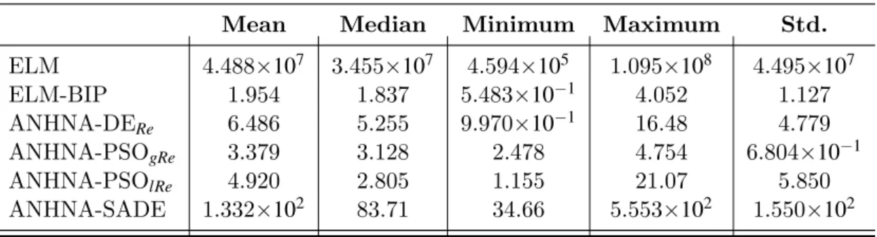
Appendix C reports tables with values of the resulting number of hidden neurons from the graphics presented in Chapter 6. We chose the following information to describe them: mean, median, maximum, minimum and standard deviation.

Appendix D reports the comparison of all variants of the proposed population-based metaheuristic approach for the ELM model selection, using all four chosen meta-heuristics. The variants with best performances were chosen to be discussed in Chapter 7. Appendix E shows typical convergence curves related to each of the independent runs of the proposed population-based metaheuristic for model selection of the ELM network, in order to illustrate how the ﬁtness values evolved through generations.

(34)

2 THE EXTREME LEARNING MACHINE

Random projections in feedforward neural networks have been a subject of interest long before the famous works of Huang, Zhu, and Siew (2004, 2006). The essence of those random projections is that the feature generation does not suffer any learning adaptation, being randomly initialized and remaining fixed. This characteristic leads to a much simpler system, where only the hidden-to-output weights (output weights for short) must be learned. In this context, the Extreme Learning Machine (ELM) arose as an appealing option for single layer feedforward neural networks (SLFN), offering a learning efficiency with conceptual simplicity.

In this chapter, Section 2.1 makes a brief review through the literature on random projections in the hidden layer of feedforward neural networks. On Section 2.2, the ELM algorithm is detailed, followed by Section 2.3, where the issues and some proposed improvements are described, such as: regularization (Subsection 2.3.1), architecture design (Subsection 2.3.2) and intrinsic plasticity (Subsection 2.3.3). At last, Section 2.4 presents

the ﬁnal remarks over this chapter.

2.1 Random projections in the literature

In 1958, Rosenblatt already stated about the perceptron theory:

A relatively small number of theorists, like Ashby (ASHBY, 1952) and von Neumann (NEUMANN, 1951; NEUMANN, 1956), have been concerned with the problems of how an imperfect neural network, containing many random connections, can be made to perform reliable. (ROSENBLATT, 1958, p. 387)

In his work, he discussed a perceptron network that responds to optical patterns as stimuli. It is formed by a set of two hidden layers, called projection area andassociation area and their connections are random and scattered. The output oﬀers a recursive link to the latest hidden layer. One of the main conclusions of this paper is:

(35)

associated to each response, they can still be recognized with a better-than-chance probability, although they may resemble one another closely and may activate many of the same sensory inputs to the system. (ROSENBLATT, 1958, p. 405)

At the end of the 1980’s, a Radial Basis Function (RBF) network with random selected centers and training only the output layer was proposed (BROOMHEAD; LOWE; LOWE, 1988, 1989 apud WANG; WAN; HUANG, 2008, 2008). This work, however, chooses the scale factor heuristically and focuses on the data interpolation. Schmidt et al. (1992) proposed a randomly chosen hidden layer, whereas the output layer is trained by a single layer learning rule or a pseudoinverse technique. It is interesting to point out that the authors did not intend to present it as an alternative learning method: “this method is introduced only to analyze the functional behavior of the networks with respect to learning.” (SCHMIDT et al., 1992, p. 1)

Pao and Takefuji (1992) presented a Random Vector Functional-Link (RVFL) which is given by one hidden layer feedforward neural network with randomly selected input-to-hidden weights (hidden weights for short) and biases, while the output weights are learned using simple quadratic optimization. The difference here lies on the fact that the hidden layer output is viewed as an enhancement of the input vector and both are presented simultaneously to the output layer. A theoretical justification for the RVFL is given in (IGELNIK; PAO, 1995), where the authors prove that RVFL is indeed universal function approximators for continuous functions on bounded and finite dimensional sets, using random hidden weights and tuned hidden neuron biases (HUANG, 2014). They did not address the universal approximation capability of a standard SLFN with both random hidden weights and random hidden neuron biases (HUANG, 2014).

(36)

followed by linear regression to estimate the output weights.

Diﬀerent works over the concept of reservoir computing were also introduced, such as Maass et al.(2002) under the notion of Liquid State Machines (LSM) and Static Reservoir Computing presented in (EMMERICH; STEIL, 2010). For more details over reservoir computing approaches and their relation to random projections considering output feedback can be found in (REINHART, 2011).

In a most recent effort on random projections, Widrow et al. (2013) proposed the No-Propagation (No-Prop), which has also a random and fixed hidden weights and only the output weights are trained. However, it uses the steepest descent to minimize mean squared error, with the Least Mean Square (LMS) algorithm of Widrow and Hoff (WIDROW; HOFF, 1960 apud WIDROW et al., 2013). Nevertheless, Lim (2013) stated that this work has been already proposed by G.-B. Huang and colleagues 10 years ago and intensively discussed and applied by other authors since.

So far, few examples of diﬀerent approaches were presented to contextualize where theExtreme Learning Machine inserts itself in the literature. The remainder of this chapter is dedicated to describe this popular network.

2.2 Introduction to ELM

As previously mentioned, ELM is a single hidden layer feedforward network with ﬁxed and random projections of the input onto the hidden state space. Proposed by Huang, Zhu, and Siew (2004, 2006), it is a universal function approximator and admits not only sigmoidal networks, but also RBF networks, trigonometric networks, threshold networks, and fully complex neural networks (WIDROW et al., 2013). Compared with other traditional computational intelligence techniques, such as the Multilayer Perceptron

(MLP) and RBF, ELM provides a better generalization performance at a much faster learning speed and with minimal human intervention (HUANG; WANG; LAN, 2011).

Given a training set with N samples {(ui,di)}N_i₌₁, where ui∈Rp is the i-th

input vector and di∈Rr is its correspondent desired output. In the architecture described

by Figure 1, with qhidden neurons and r output neurons, thei-th output at time stepk is given by

(37)

Figure 1 – Extreme Learning Machine architecture, where only the output weights are trained.

Source: author.

whereβ ∈Rq×r is the weight matrix connecting the hidden to output neurons.

For each input pattern u(k), the correspondent hidden state h(k)∈Rq is given by

h(k) =f mT₁u(k) +b1

. . . f mT_qu(k) +bq

, (2.2)

wheremj∈Rp is the weight vector of the j-th hidden neuron and is initially drawn from

a uniform distribution, remaining unaﬀected by learning. The bj is its bias value and

f(·)is a nonlinear piecewise continuous function satisfying ELM universal approximation capability theorems (HUANG et al., 2006 apud HUANG, 2014, p. 379), for example:

1. Sigmoid function:

f(·) = 1

1+expa(mT_ju(k)) +bj

(38)

2. Hyperbolic tangent:

f(·) =

1−exp

−a(mT_ju(k)) +bj

1+exp

−a(mT_ju(k)) +bj

(2.4)

3. Fourier function:

f(·) =sin mT_ju(k) +bj

(2.5)

4. Hard-limit function:

f(·) =

 



1 if mT_ju(k) +bj

≥0

0 otherwise

(2.6)

5. Gaussian function:

f(·) =exp −bjku(k)−mjk2

(2.7)

wherea is the function’s slope, usually ignored being set to 1. Let the hidden neurons output matrix be described by:

H=



   

h1(1) ... hq(1)

... . .. ...

h1(N) ... hq(N) 

   

N×q

. (2.8)

The output weights β is given by the solution of an ordinary least-squares (see Equation 2.9).

Hβ =D, (2.9)

where D∈RN×r is the desired output matrix. This linear system can simply be resolved by least-squares method, that in its batch mode, is computed by

β =H†D (2.10)

whereH†= HTH−1HT is the Moore-Penrose generalized inverse of matrix H. Diﬀerent methods can be used to calculate Moore-Penrose generalized inverse of a matrix, such as orthogonal projection method, orthogonalization method, singular value decomposition (SVD) and also through iterative methods (HUANG, 2014). In this work, the SVD

approach was adopted.

(39)

Algorithm 1: Extreme Learning Machine

1: Training set{(ui,di)}N

i=1 withu∈Rp and d∈Rr;

2: Randomly generate the hidden weightsM∈Rp×q and biasesb∈Rq;

3: Calculate the hidden layer output matrixH;

4: Calculate the output weight vectorβ (see Equation 2.10);

5: returnβ.

2.3 Issues and improvements for ELM

Even though ELM networks and its variants are universal function approx-imators, their generalization performance is strongly influenced by the network size, regularization strength, and, in particular, the features provided by the hidden layer (NEUMANN, 2013). One of the issues inherited from the traditional SLFN is how to obtain the best architecture. It is known that a network with few nodes may not be able to model the data, in contrast, a network with too many neurons may lead to overfitting (MARTÍNEZ-MARTÍNEZ et al., 2011). Another shortcoming is that the random choice of hidden weights and biases may result in an ill-conditioned hidden layer output matrix, which derails the solution for the linear system used to train the output weights (WANG

et al., 2011; HORATA et al., 2013). An ill-conditioned hidden layer output matrix also provides unstable solutions, where the small errors in the data will lead to errors of a much higher magnitude in the solution (QUARTERONI et al., 2006, p. 150). This is reﬂected on the high norm of output weights, which is not desirable as discussed in the works of Bartlett (1998) and Hagiwara and Fukumizu (2008), where they stated that the size of output weight vector is more relevant for the generalization capability than the conﬁguration of the neural network itself. This can be observed as the training error enlarges and the test performance deteriorates (WANG et al., 2011). To deal with this, ELM uses SVD even though it is computationally consuming.

In the following subsections, we presented some works and proposed improve-ments for ELM network that concerns the aforementioned issues.

2.3.1 Tikhonov’s regularization

(40)

encountered when there is not a distinct output for every input, when there is not enough information in the training set that allows a unique reconstruction of the input-output mapping, and the inevitable presence of noise or outliers in real-world data which brings uncertainty to the reconstruction process (HAYKIN, 2008, chap. 7).

To deal with this limitation, it is expected that some prior information about the mapping is available. The most common form of prior knowledge involves the as-sumption that the mapping’s underlying function is smooth, i.e., similar inputs produce similar outputs (HAYKIN, 2008, chap. 7). Based on that, the fundamental idea behind regularization theory is to restore well-posedness by appropriate constraints on the solution, which contains both the data and prior smoothness information (EVGENIOUA et al., 2002).

In 1963, Tikhonov introduced a method named Regularization (TIKHONOV, 1963 apud HAYKIN, 2008, chap. 7), which became state of the art for solving ill-posed problems. For the regularized least-squares estimator, its cost function for the i-th output neuron is given by

J(β_i) =kεik2+λkβik2, (2.11)

kεik2=εTi εi= (di−Hβi) T

(di−Hβi). (2.12)

where εi∈RN is the vector of error between the desired output and the network’s output,

and λ >0 is the regularization parameter.

The ﬁrst term of the regularization cost function is responsible for minimizing the error squared norm (see Equation 2.12), enforcing closeness to the data. The sec-ond term of this function minimizes the norm of the output weight vector, introducing smoothness, while λ controls the trade-oﬀ between these two terms.

Minimizing Equation 2.11, we obtain

ˆ

β_i= HTH+λI−1HTdi, (2.13)

(41)

2.3.2 Architecture optimization

As previously mentioned, one of the issues of the ELM network is to determine its architecture. On one hand, few hidden neurons may not provide enough information processing power and, consequently, a poor performance. On the other hand, a large hidden layer may create a very complex system and lead to overﬁtting. To try to handle this issue, three main approaches are pursued (XU et al., 2007; ZHANG et al., 2012):

• constructive methods start with a small network and then gradually adds new hidden

neurons until a satisfactory performance is achieved (HUANG et al., 2006; HUANG; CHEN, 2008; HUANG et al., 2008; FENG et al., 2009; ZHANG et al., 2011; YANG

et al., 2012);

• destructive methods also known as pruning methods, start by training a much larger

network and then removes the redundant hidden neurons (RONGet al., 2008; MICHE

et al., 2008; MICHEet al., 2011; FAN et al., 2014);

• evolutionary computation uses population-based stochastic search algorithms that are

developed from the natural evolution principle or inspired by biological group behavior (YAO, 1999). Besides the adaptation of an architecture, they may also perform weight and learning rule adaptation, input feature selection, weight initialization, etc (YAO, 1999). More about architecture design with metaheuristics is further described

in Chapter 4 and some metaheuristics algorithms are detailed in Appendix A. Huang et al. (2006) proved that an incremental ELM, named I-ELM, still maintain its properties as universal approximator. In 2008, two approaches were proposed to improve I-ELM performance. In (HUANGet al., 2008), the I-ELM was extended from the real domain to the complex domain with the only constraint that the activation function must be complex continuous discriminatory or complex bounded nonlinear piecewise continuous. Also, in 2008, Huang and Chen proposed an enhanced I-ELM, named EI-ELM. It diﬀers from I-ELM by picking the hidden neuron that leads to the smallest residual error at each learning step. This resulted in a more compact architecture and faster convergence.

Still on constructive methods, the Error Minimized Extreme Learning Machine

(EM-ELM) (FENG et al., 2009) grows hidden neurons one by one or group by group, updating the output weights incrementally each time. Based on EM-ELM, Zhang et al.

(42)

with better performance instead of keeping the existing ones. The output weights are still updated incrementally just as EM-ELM. Yang et al. (2012) proposed the Bidirectional Extreme Learning Machine (B-ELM), in which some neurons are not randomly selected and takes into account the relationship between the residual error and the output weights to achieve a faster convergence.

On pruning methods, we can mention the Optimally Pruned Extreme Learning Machine (OP-ELM) (MICHE et al., 2008; MICHE et al., 2010), that starts with a large hidden layer, then each hidden neuron is ranked according with a Multiresponse Sparse Regression Algorithm and, ﬁnally, neurons are pruned according to a leave-one-out cross-validation. TROP-ELM (MICHE et al., 2011) came as an OP-ELM improvement, that adds a cascade of two regularization penalties: ﬁrst a L1 penalty to rank the neurons of the hidden layer, followed by a L2 penalty on the output weights for numerical stability and better pruning of the hidden neurons. Finally, and most recently, the work of Fan

et al. (2014) proposes an Extreme Learning Machine withL₁_/₂ regularizer (ELMR), that identiﬁes the unnecessary weights and prunes them based on their norms. Due to use of the L₁_/₂ regularizer, it is expected that the absolute values of the weights connecting relatively important hidden neurons become fairly large.

Although constructive and pruning methods address the architecture design, they explore only a limited number of available architectures (XU; LU; HO, 2007; ZHANG et al., 2012). As mentioned above, evolutionary algorithms allows that not only the architecture (number of layers, number of neurons, connections, etc) but also activation functions, weight adaptation and others to be optimized. Because of this feature, we adopted this method in this work and will be further detailed in Chapter 4.

2.3.3 Intrinsic plasticity

(43)

Biologically, this phenomenon helps neurons maintain appropriate levels of electrical activity, by shifting the positions and/or the slopes of the response curves to make the sensitive regions of the response curves always correspond well with input distributions (LI, 2011). Even though it is still uncertain how the underlying processes work, there is experimental evidence suggesting that it plays an important role as part of the memory engram1 _{itself, as a regulator of synaptic plasticity underlying learning and memory, and} as a component of homeostatic regulation (CUDMORE; DESAI, 2008).

Baddeley et al (1997) (BADDELEY et al., 1997 apud LI, 2011) performed an experimental observation where they concluded that neurons exhibit approximately exponential distributions of the spike counts in a time window. Based on this information, computational approaches were developed to study the eﬀects of intrinsic plasticity (IP) on various brain functions and dynamics.

In a mathematical manner, their goal is to obtain an approximately exponential distribution of the firing rates. Since the exponential distribution has the highest entropy among all distributions with fixed mean (TRIESCH, 2005), those approaches attempt to maximize the information transmission while maintaining a fixed average firing rate, or equivalently, minimize their average firing rate while carrying a fixed information capacity (LI, 2011). As examples, we may cite: (BELL; SEJNOWSKI, 1995), (BADDELEY et al., 1997), (STEMMLER; KOCH, 1999), (TRIESCH, 2004), (SAVIN et al., 2010) and (NEUMANN, 2013).

Triesch (2005) proposed a gradient rule for intrinsic plasticity to optimize the information transmission of a single neuron by adapting the slopeaand biasbof the logistic sigmoid activation function (see Equation 2.3) in a way that the hidden neurons’ outputs become exponentially distributed. Based on his works (TRIESCH, 2004; TRIESCH, 2005; TRIESCH, 2007), Neumann and Steil (2011) proposed a method named Batch Intrinsic Plasticity (BIP) to optimize ELM networks’ hidden layer. The diﬀerence between those two methods lies on the parameters a and b estimation that, in BIP, the samples are presented all at once and the parameters are calculated in only one shot.

Since ELM has random hidden weights, they may lead to saturated neurons or almost linear responses which may also compromise the generalization capability (NEUMANN; STEIL, 2013). Nevertheless, this can be avoided using activation functions

1